Assessing ecosystem integrity by monitoring populations and communities is an important management tool, but is often limited by the immense variety of species and the rarity of many of them. Grouping species by their responses to variation in the environment is one approach to choosing species to serve as effective indicators of community change. Moreover, identifying species that are characterized by similar archetypical responses to the environment increases the power to predict their occurrence and simplifies management of diverse species assemblages by focusing on a much smaller number of archetypes. To this end, we used the species archetype model (SAM) to fit generalized linear models of environmental covariates to species distribution data in order to identify environmentally correlated groups of kelp forest species in the Santa Barbara Channel region. Eighty-two species of macroalgae, invertebrates, and fish monitored in kelp forests across the channel were grouped into one of 10 archetypes based on their similar responses to environmental parameters, with water temperature emerging as one of the strongest drivers of archetype differences. Predictive maps of the distribution of species archetypes identified sites where multiple archetypes are common, indicating high diversity, as well as sites where rare species are more likely to occur. Potential indicator species were identified for each archetype. New monitoring efforts across the growing Marine Biodiversity Observation Network could use modeling approaches like SAM to guide their designs, optimizing the cost-to-​benefit ratio of monitoring whole communities.

Giant kelp (Macrocystis pyrifera), Channel Islands National Marine Sanctuary (CINMS), California. Photo credit: Robert J. Miller, University of California Santa Barbara. > High res figure

Introduction

The idea that environmental management should consider the ecosystem or landscape as a whole is decades old and has spawned entire branches of ecology (Slocombe, 1993; Grumbine, 1994). In practice, however, ecosystem-based management is often stymied by a combination of sociopolitical obstacles and practical difficulties in connecting ecological principles with concrete goals and ways to measure progress towards them (Arkema et al., 2006; Levin et al., 2009). The challenges to implementing ecosystem-based management are particularly problematic in marine systems, where this management approach may offer a way to reverse widespread declines in coastal and oceanic ecosystems and in the functions and services they provide (Leslie and McLeod, 2007). Despite this potential, marine ecosystem-based management lags behind its terrestrial counterpart in implementation (Townsend et al., 2018). Largely focused on fisheries, marine management instead relies heavily on single-species population dynamics or habitat suitability models, despite the wealth of ecological research showing the importance of entire communities and biodiversity on ecosystem structure and function (Thrush et al., 2016). An important exception to this has been marine protected areas, which aim for ecosystem-based management by protecting all components of the ecosystem rather than by explicit consideration of multispecies dynamics. More sophisticated approaches to marine ecosystem-based management, such as adaptive management of sites over time, have been limited by the difficulty of predicting and detecting ecological change in diverse ecosystems that are inherently difficult to access and observe (Barbier et al., 2008; Ellingsen et al., 2017).

Addressing the challenge of implementing ecosystem-based management in marine habitats would be more tractable if entire communities could be monitored and modeled. While improved survey techniques could help with this, another route to ecosystem-based management is to focus on strategically chosen indicator species that yield information about larger segments of the ecological community. Yet, ecologists still debate to what extent communities are conglomerations of species reacting individually according to their environmental preferences or to random processes (Gleason, 1926; Hubbell, 2005) versus tightly interacting groups of species that replace each other across environmental gradients (Clements, 1916; Whittaker, 1975; Shipley and Keddy, 1987). In the latter case, cohesive groups of species would be expected to respond to gradients of environmental parameters in similar ways (Leaper et al., 2014). Identifying such groups of closely associated species could greatly facilitate modeling of multi­species dynamics and ecosystem management by reducing the number of variables, and would provide insight into the identity and composition of natural communities. If indicator or surrogate species representing groups could be identified, then they could be used to track the status of the whole group, reducing the cost and difficulty of community-level monitoring (Carignan and Vilard, 2002; Caro, 2010; Siddig et al., 2016). These factors are particularly advantageous for rare species, which represent the majority of species in most communities (Magurran and Henderson, 2003; Gaston and Blackburn, 2008) and require much more effort to observe and effectively sample (Ricklefs, 2000; MacKenzie et al., 2005; Thompson, 2013). Ideally, indicator species for such archetypes would be more common and easier to monitor, but monitoring a few key rare species is still easier than monitoring all of them.

Indicator species have a long history of use for monitoring ecosystem or environmental health and integrity, habitat restoration, and assessing the effects of human impacts such as pollution and contamination. A review by Siddig et al. (2016) found that indicators were generally chosen based on a posteriori information from the literature, local abundance, ecological significance, or conservation status. Indicator species, moreover, are often chosen purely to increase the efficiency of monitoring rather than to improve specific management decisions (Bal et al., 2018). If management interest centers on biodiversity and communities, selecting indicator species that track those communities would be desirable.

Species archetype models (SAM; Dunstan et al., 2011) have been used successfully to identify environmentally correlated groups of species by fitting a mixture of generalized linear models of environmental covariates to species distribution data (Woolley et al., 2013; Murillo et al., 2018, Contreras 2019). Identifying species that are characterized by a limited number of archetypical responses to the environment increases the predictive power of the SAM across species and simplifies management considerations for diverse species assemblages to a much smaller number of archetypes or species groups (Dunstan et al., 2011; Hui et al., 2013). Additional advantages of the SAM include its ease of use for predicting community responses to the environment and the information it provides about community assembly based on the degree of overlap or separation of the archetypes and the number of species in each archetype (Leaper et al., 2014). Identifying archetypes makes it possible to identify surrogate species (Lindenmayer et al., 2015; Tulloch et al., 2016) that are common or easy to identify and can be used as proxies for archetypical units as a whole, particularly when they can give information about the status of co-occurring rare species. SAMs can also be used to predict how communities respond to environmental change based on species-specific information (Hui et al., 2013). Such predictions are typically challenging using traditional correlational approaches due to a lack of information for many species, particularly those that are uncommon or rare. By pooling information from species within an archetype, the SAM can overcome these challenges and generate more accurate predictions of species occurrence than individual species distribution models (Hui et al., 2013).

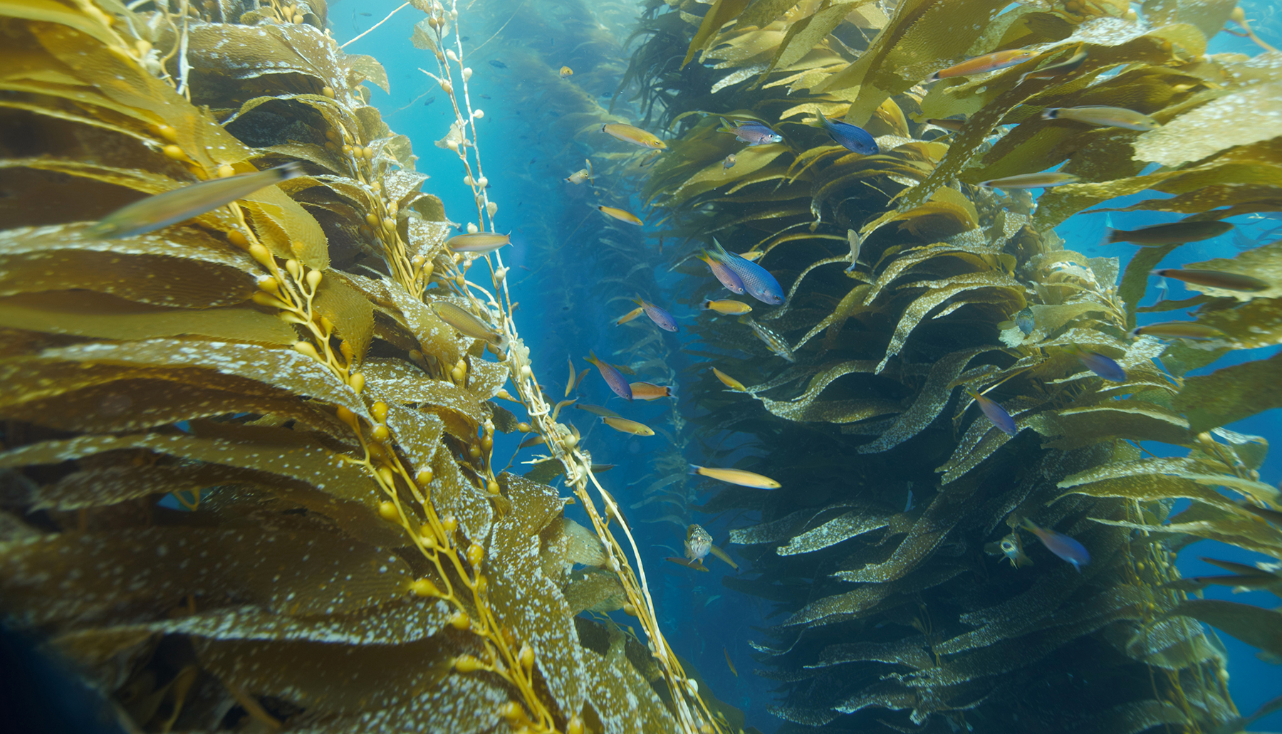
The northern Channel Islands in the Southern California Bight are located at the boundary between the Oregonian and Californian marine provinces, where strong environmental gradients have long been considered to affect regional biodiversity (Hewatt, 1946). Complex circulation patterns around the islands are driven by the collision of the California Current, which produces seasonal upwelling, with the warmer Southern California Countercurrent (Hickey, 1992; Hendershott and Winant, 1996; Harms and Winant, 1998). Giant kelp (Macrocystis pyrifera) is abundant on shallow coastal reefs surrounding the islands, forming forests that harbor diverse subtidal communities that are influenced by a multitude of physical and biological processes (see Schiel and Foster, 2015, for a review). Broad appreciation of and interest in the ecological importance and economic value of the Channel Islands kelp forests led to the establishment of a network of marine protected areas (MPAs) there. Ongoing research and monitoring programs established by the US National Park Service (NPS), the Partnership for Interdisciplinary Studies of Coastal Oceans (PISCO), and the Santa Barbara Coastal Long Term Ecological Research program (SBC LTER) provide more than three decades of data on the community structure and dynamics of these systems and the physical and biological processes that structure them (Kushner et al., 2013; Lamy et al., 2018; Menge et al., 2019).

Here, we apply species archetype modeling to a spatially and temporally extensive data set that shows the occurrence of kelp forest species at the Channel Islands to: (1) identify groups of species with similar responses to environmental covariates, as well as indicator species that could potentially serve as surrogates for entire archetypes, to inform management; (2) evaluate the utility of the model for predicting the species composition of kelp forest communities; and (3) predict patterns of species occurrence at unsampled sites in the region. To test the robustness of our approach, we compared our model predictions of species occurrence based on data collected by the NPS to occurrence patterns observed in a separate data set collected by PISCO.

 

Methods

Biological Data

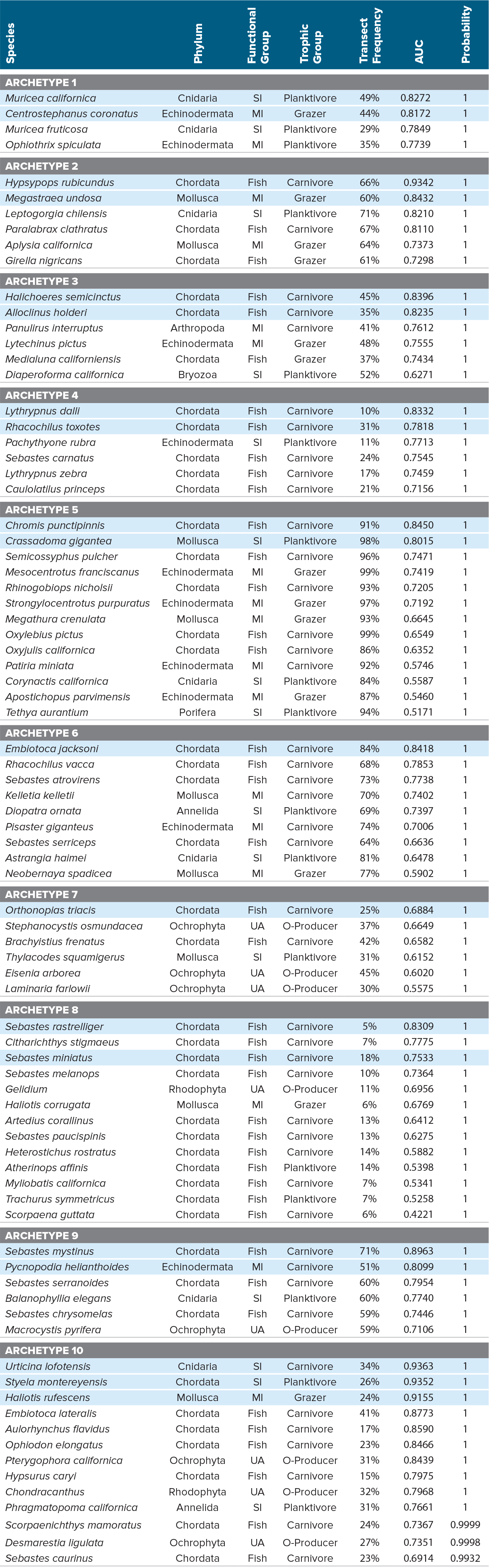
Kelp forest monitoring program. The NPS surveys subtidal rocky reef communities to measure abundances of macroalgae, invertebrates, and fish at 33 sites across five of the northern Channel Islands for the Kelp Forest Monitoring Program (KFMP; Kushner et al., 2013). Surveys include visual counts of larger algae, invertebrates, and fish, as well as point contact assessments of sessile benthic flora and fauna. Though KFMP surveys began in the early 1980s, we used data from 2004 to 2014 to retain consistency of sampling protocols and availability of data on environmental covariates. We constrained our analyses to 82 species (Table 1) that were identified to the species level and were present in at least 5% of the KFMP surveys. These data were used to parameterize the SAMs and for initial model assessment.

 

Table 1. Species list with archetype assignment and species-level AUC ROC (area under the receiver operating characteristic curve). Functional groups are understory algae (UA), sessile invertebrates (SI), mobile invertebrates (MI), and fish. Transect Frequency represents the percent of transects in which the species occurred, across all sites and years. Potential indicator species for each archetype are highlighted with blue shading and represent the top 1–3 conspicuous species predicted by the model. The probability column shows the archetype membership probability for each species. > High res table

 

PISCO kelp forest monitoring program. Kelp forest community data collected by PISCO from 2004 to 2014 were used to test the robustness of SAMs derived from the KFMP data set. We used PISCO data for the same 82 species retained from the KFMP data set collected from 45 sites. Data were collected using methods similar to those used by KFMP, with some differences in size and spatial distribution of replicates (Carr et al., 2020; Malone et al., in press). The PISCO sites used in this analysis are distributed across a geographic area that encompasses four of the northern Channel Islands as well as mainland California sites, and so includes the region surveyed by the KFMP as well as a nearby stretch of the mainland coast of the Santa Barbara Channel (Figure 1). All data are publicly available (Carr et al., 2020; SCB MBON 2021a,b,c,d).

 

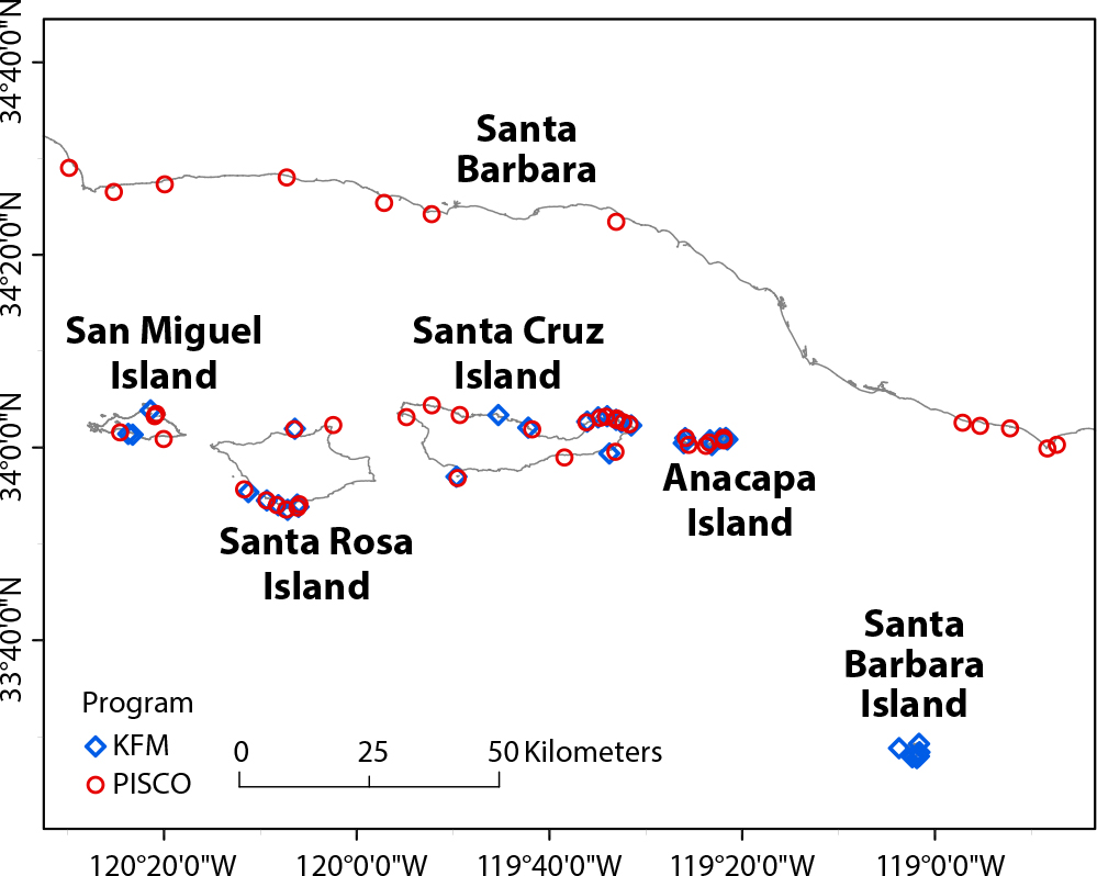
Figure 1. Map of the Santa Barbara Channel and northern Channel Islands. Channel Islands National Park Kelp Forest Monitoring Program (KFMP) subtidal sampling sites are marked with blue diamonds, and Partnership for Interdisciplinary Studies of Coastal Oceans (PISCO) sites are marked with red circles. > High res figure

 

Environmental Covariates

We selected environmental variables known or hypothesized to affect kelp forest community structure (reviewed in Schiel and Foster, 2015) as SAM covariates (Table S1). At the transect level, mean water depth and coverage of rock substrate were measured by KFMP and PISCO divers using a point contact method. Sea surface temperature (SST) values were estimated using the Group for High Resolution Sea Surface Temperature (GHRSST) Level 4 Global Foundation Sea Surface Temperature Analysis data set (JPL MUR MEaSUREs Project, 2015, version 4.1). This data set combines the SST measurements from multiple instruments into a gridded data set with a 0.01° spatial resolution (approximately 1 km) and one-day temporal resolution. We interpolated a two-dimensional surface using the R package akima (Akima et al., 2016) and extracted daily temperature values for each of the sites. To match the annual sampling scale of the biological survey data, we generated annual SST summary statistics, specifically seasonal means and the mean temperature in the hottest and coldest months. Year was also used as a continuous covariate.

Sea surface chlorophyll a concentration (Chl-a) was estimated using the Kahru et al. (2012, 2015) merged California Current 1 km data set, available at http://www.wimsoft.com/CAL/. This data set incorporates ocean color data from multiple satellite sources and can outperform estimates derived from single satellites in the region when compared to in situ Chl-a measurements (Kahru et al., 2012). Significant wave height data were estimated using the Coastal Data Information Program (CDIP, http://cdip.ucsd.edu) MOnitoring and Prediction (MOP) model (v1.1) for Southern and Central California (O’Reilly et al., 2016). Briefly, the model uses directional wave data from CDIP’s network of sensor buoys to initialize a spectral wave propagation model. The outputs are high resolution (hourly 100 m × 100 m) estimates of significant wave height and wave period. We used both mean and maximum significant wave height variables. Turbidity was estimated using the NOAA diffuse attenuation (K490) data set available from https://coastwatch.pfeg.noaa.gov/erddap/griddap/erdMWk490mday.html.

At the regional scale, we incorporated annual mean values of three regional climatic indices: the Multivariate El Niño Index (MEI, https://psl.noaa.gov/enso/mei/), the North Pacific Gyre Oscillation (NPGO, http://www.o3d.org/npgo/npgo.php), and the Pacific Decadal Oscillation (PDO, http://research.jisao.washington.edu/​pdo/PDO.latest.txt).

To avoid effects of multicollinearity, we examined the environmental covariates using Spearman’s correlations and Variance Inflation Factors (VIF). In cases where covariates had Spearman’s correlation coefficients >0.7, we built single covariate SAMs with each of them and retained the covariate with the lowest model Bayesian Information Criterion (BIC) to reduce the VIF below an a priori threshold of 3. All environmental covariates were scaled (mean = 0, standard deviation = 1) to avoid effects from differences in dimensions.

 

Model Fitting and Evaluation

Species archetype models were generated using the mixture model method developed by Dunstan et al. (2011) and implemented in the SpeciesMix (Dunstan et al., 2016) package. Fitting the SAM is a two-step process. First, we chose the number of archetypes by fitting the full model (including all covariates) with a varying number of archetypes, ranging from a model where all species were assigned to a single archetype up to a model with 20 archetypes. The final number of best-fitting archetypes was selected using the Bayesian Information Criteria (BIC; Dunstan et al., 2011).

Once the best number of archetypes had been selected in a model that included all environmental variables, more parsimonious SAMs were constructed through stepwise removal of environmental covariates. The BIC for each model was used to identify which variables should be removed, and ultimately to determine the best combination of covariates.

We calculated the area under the receiver operating characteristic curve (AUC ROC) using the R package modEvA (v. 1.3.2; Barbosa et al., 2016) and used this metric to evaluate the discriminatory power of the final model. Evaluating the model on KFMP data was valuable, because it measured the degree to which SAMs retain predictive ability despite collapsing the species into a limited number of archetypes, but it had the disadvantage of testing performance on data that were also used to fit the model. A stronger test of its utility is to confront the model with new data, testing whether it can predict the presence of species at new locations based only on environmental data. For this purpose, we compared our predictions to species occurrence data from the same region collected by PISCO using similar methods.

 

Regional Predictions

We used the final SAM to predict the probability of the presence of each archetype throughout the Santa Barbara Channel using environmental conditions in 2014. Environmental covariates were estimated as described above, except for depth and rock coverage, which were measured directly within the sampled plots surveyed by divers, but had to be derived from other sources for the continuous regional predictions. Depth was estimated throughout the region using the NOAA National Geophysical Data Center 1/3 arcsecond digital elevation models for the Santa Barbara and Santa Monica regions (https://catalog.data.gov/​dataset/​santa-​barbara-​california-​coastal-​digital-​elevation-​model). There are no comprehensive maps of substrate cover for the region, so we used presence of giant kelp (Macrocystis pyrifera) canopy as a proxy for presence of hard substrate (Rassweiler et al., 2012). Data on kelp canopy presence at 30 m spatial resolution were derived from Landsat 5 Thematic Mapper and Landsat 7 Enhanced Thematic Mapper+ satellite images (Bell et al., 2020). We restricted our predictions to locations within the depth range of the kelp forest monitoring sites (between 3.5 m and 27 m) and within 50 m of areas where a patch of giant kelp was remotely observed between 2005 and 2014 as an indicator of sufficient rocky substrate to support the kelp forest species used in our analyses.

 

Results

Model Description

We initially evaluated model performance with numbers of archetypes ranging from 1 to 20. Based on the resulting BIC values, we chose to proceed with the 10-archetype model, beyond which additional archetypes offer minimal improvements in BIC (Figure S1; Dunstan et al., 2011). We then removed environmental covariates from the 10-archetype model in a stepwise fashion and examined the change in BIC to identify the best combination of environmental covariates. Our most likely model included 12 environmental parameters as covariates and predictors of species presence/absence (Figures 2 and S2). The mean and variation in sea surface temperature (SST, CV SST), and to a lesser extent maximum wave height, chlorophyll a, and turbidity, were the most influential covariates (Figures 2 and S3). Archetypes 1–3 were associated with warm water, while archetypes 9–10 were cold water archetypes (Table 1, Figure 2).

 

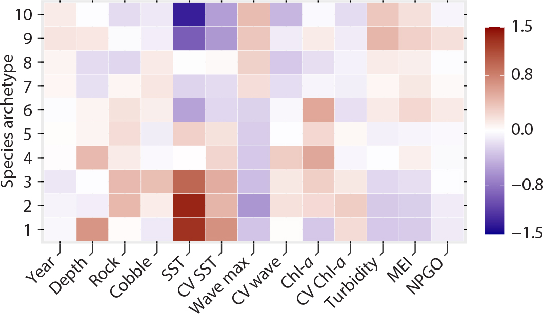
Figure 2. Model coefficients for environmental variables by archetype for most the parsimonious species archetype models (SAMs). Archetypes are assigned identification numbers, which are arbitrary but consistent throughout the paper. > High res figure

 

Archetype Composition

The estimated archetype membership probability for all species was high (>0.90, Table 1), indicating good agreement between the species response to the environmental covariates and predicted archetype responses. Most archetypes contain diverse groups of organisms with no clear patterns with respect to taxonomic group or trophic level (Table 1). Some phylogenetic clustering was evident in archetype 4, which consists almost entirely of fish, and archetype 5, which contains four of the nine echinoderm species in the data set. Species with similar frequency of occurrence in the surveys tended to group within archetypes. Archetype 5 contained species that were common (i.e., occurred in >84% of surveys) across the region, while species in archetype 8 were relatively uncommon (i.e., occurred in <18% of surveys).

 

Model Performance

Model performance was evaluated using the area under the receiver operating characteristic curve (AUC ROC). The overall model had an AUC ROC of 0.87 (note that 0.50 represents performance if presence/absence were assigned at random, and 1.0 represents perfect accuracy). Individual species AUC ROCs were all above 0.5 with one exception (Scorpaena guttata; at 0.33), and 68% (55 out of 82 species) had AUC values >0.7. Thus, the approach produces consistently useful results.

A strong test of a model of community composition is to ask if it can predict species occurrence in a new data set, collected with different methods. We found the model retained considerable utility when used to predict species presence at sites sampled by PISCO (Figure 3). Model testing with the PISCO data set resulted in a similar, though lower, AUC ROC (0.72). As expected, model accuracy was somewhat lower on this novel data than on the KFMP data set on which it was trained. Nevertheless, model predictions were informative (i.e., AUC >0.5) for more than 73% of species, even in this independent data. To examine if the mainland sites included in the PISCO data set were mainly responsible for the lower AUC, we also ran the model on the inland and mainland sites separately (Figure S4). The mainland model had a slightly lower AUC (0.695) than the island sites (0.73).

 

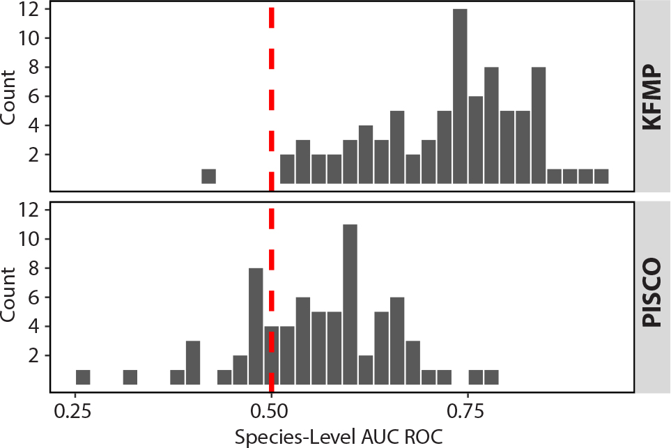
Figure 3. Comparison of area under the receiver operating characteristic curve (AUC ROC) by species for the KFMP and PISCO data sets. The red dotted line represents the 0.5 predictive threshold ROC. > High res figure

 

Regional Map Predictions

Regional prediction maps, generated for 2014 environmental conditions, showed that three to seven species archetypes were likely (>50% probability) to be present at each site (Figure 4). There was a non-zero probability of occurrence for all archetypes at all sites considered (Figure 5), but some archetypes had low prevalence. For example, archetype 8 was <10% likely to be present at most (59%) locations. This archetype contains species that are consistently rare throughout the region at the site scale (Table 1). Conversely, archetype 5 is composed of species that occur frequently in the region (Table 1) and has a high probability (>90%) of presence at 92% of the sites (Figure 5). This suggests that the species in these two archetypes do not have strong responses to the environmental covariates considered, which is consistent with their generally near-zero model coefficients (Figure 2). Archetypes 1–3 had strong positive responses to temperature (Figure 2), and consequently had higher probabilities of occurrence at the eastern end of the Santa Barbara Channel, where temperatures are warmer (Figure 5). Archetypes 9 and 10 exhibit the inverse pattern, higher probability of occurrence at the western end of the region (Figure 5), corresponding to their negative correlation with temperature and positive correlation with wave energy (Figure 2).

 

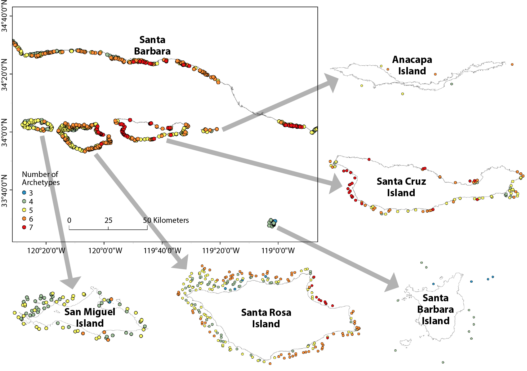
Figure 4. Regional estimates of the number of archetypes present at each location based on 2014 conditions. Species archetypes greater than 50% probability of presence are included in this map. The range of species archetypes at each location is between three and seven (shown in legend). > High res figure

 

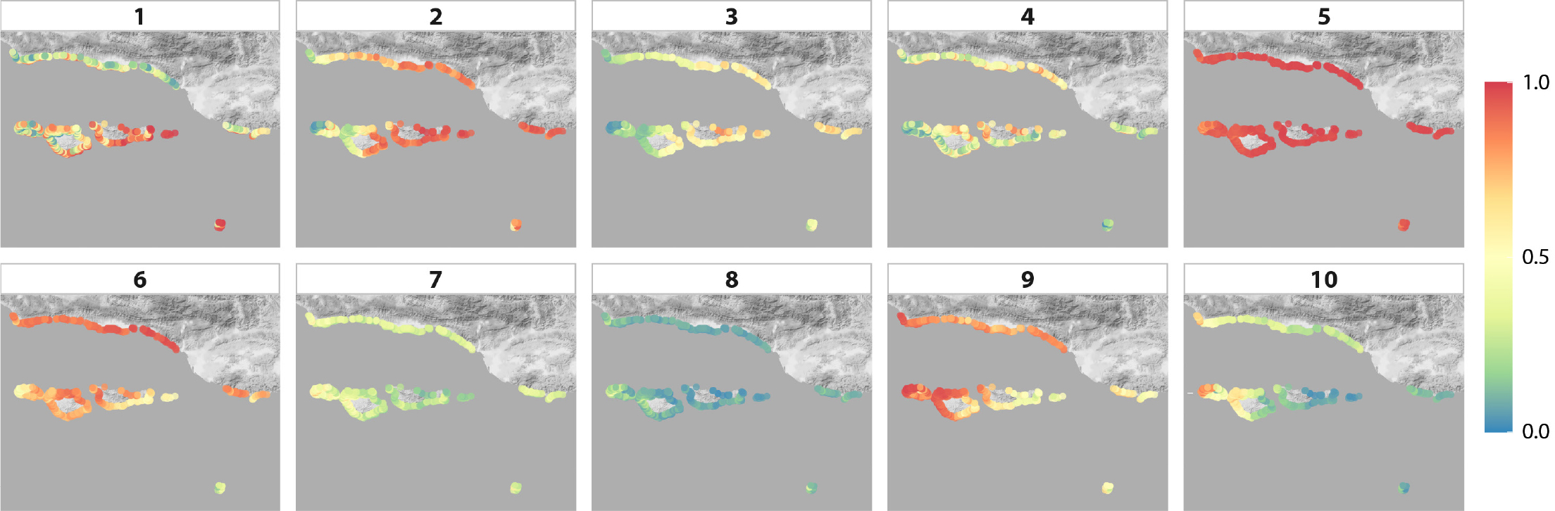
Figure 5. Maps of predicted occurrence of each of the 10 modeled species archetypes across the Santa Barbara Channel, based on 2014 conditions. The scale corresponds to the probability of occurrence. > High res figure

 

Discussion

The 82 species of macroalgae, invertebrates, and fish monitored in kelp forests across the Santa Barbara Channel fell into 10 archetypes, each comprising groups of species that had similar responses to environmental parameters. Half of the archetypes were strongly driven by water temperature, with three characterized by warm conditions and two by cold. The utility of the archetypes for providing surrogates for monitoring rare species was somewhat undermined by the fact that many uncommon species grouped together. Nevertheless, we could identify indicator species for these groups that are easy to detect. For example, archetype 8 was dominated by species occurring in ≤14% of surveys, but was best characterized by the presence of Sebastes rastrelliger, the grass rockfish, a conspicuous and easily counted species. Predictive maps of the distribution of species archetypes identified sites where multiple archetypes are likely common, suggesting high diversity, such as the zone between Santa Cruz and Santa Rosa Islands (Figure 4), as well as sites where rare species are more likely to occur (Figure 5). These results could be used to guide future monitoring and predictive efforts in the region, as well as management. Even the best marine monitoring programs have gaps between sampling locations, so managers are regularly forced to make decisions for such unmonitored locations; model predictions would provide useful information in such circumstances.

Although the mosaic of species responses was dominated by the strong SST gradient in the region, wave height, chlorophyll a, and turbidity were also important predictors, and the additional covariates substantially improved the predictive power of the model. The observed importance of temperature agrees with previous work in the region identifying SST as a dominant environmental gradient that structures subtidal communities (Lamy et al., 2018), and with a global analysis showing the primacy of SST as a predictor of marine biodiversity (Tittensor et al., 2010). The importance of wave height was also expected, particularly because it is known to influence giant kelp (Reed, 2011; Bell et al., 2015), a foundation species with cascading effects on rocky reef ecosystems (Miller et al., 2018; Lamy et al., 2020; Detmer et al., 2021). Although we could have included giant kelp abundance itself in the model, we opted to use kelp as one of the response variables rather than as a predictor because preliminary analyses suggested it would not have been a strong predictor. Chlorophyll a is in an indicator of phytoplankton, which support zooplankton and reef suspension feeders that in turn are prey for mobile invertebrates and fishes (Page et al., 2013). Turbidity may affect benthic communities by reducing light, a vital resource for benthic macrophytes (Miller et al., 2011). Climate change is predicted to affect all of these variables. Transient warming effects associated with El Niño and the warm “blob” event in 2013–2015 were observed in the region (Cavole et al., 2016; Reed et al., 2016), and such events may increase in frequency and intensity in the future (Di Lorenzo et al., 2016). Climate change is also predicted to alter the frequency and intensity of storms and waves in the Pacific, with increases in intense cyclones in the North Pacific (Graham and Diaz, 2001; Ulbrich et al., 2009). Interestingly, archetypes 1–3, characterized by warm water, tended to be negatively affected by maximum wave height, and the cold-water archetypes, 9 and 10, were positively associated with maximum wave height, suggesting conflicting effects of climate change on archetype dominance. Nevertheless, the temperature coefficients were much larger, and we predict that archetypes 1–3 will become more prevalent to the extent that the Santa Barbara Channel is increasingly impacted by marine heatwaves in the future.

Predictive performance varied across species, but SAMs were generally useful for predicting species presence. Strikingly, the model developed using data from KFMP had considerable ability to predict species occurrence at different locations in the region monitored by PISCO. Although accuracy was lower when the model was confronted with PISCO data, it is still impressive given differences in sampling methodology between the two programs. For example, KFMP samples fish in timed swims where a diver roves over a 2,000 m² area, while PISCO samples in more traditional 60 m² transects, yielding significantly different estimates of fish species diversity (Rassweiler et al., 2020). Furthermore, the PISCO data set includes mainland sites outside the area where training data were collected (Figure 1), although the similar AUC scores for separate mainland and island models (Figure S4) suggest that the survey methods made more of a difference that the geographic distribution of sites.

Although the approach offered useful predictions for most species, there were several species for which predictions of distributions were less reliable. Several explanations may apply to these cases. First, the SAM approach relies on generalized linear models (GLMs) to describe the relationship between species distributions and environmental covariates. For some species, this relationship may be nonlinear, and thus difficult to fit with a GLM. A second potential cause of poor performance is the lack of inclusion of key covariates. Though an extensive suite of covariates were considered here, other environmental factors, including variation in larval delivery and habitat stability, have been shown to affect distributions of some species; for example, Storlazzi et al. (2013) found higher abundances of the sea star Patiria minata in more stable environments. The mechanism by which covariates affect species distributions also likely varies by species, and the way a specific covariate is included may not encompass species-specific mechanisms. For example, average SST in the coldest month preceding the biological survey, was selected from multiple SST summary variables (e.g., seasonal means, annual mean) as the best-performing SST variable for the full model. However, for individual species, the mechanism could involve a specific SST threshold that may not be well represented by SST in the coldest month, leading to poor predictive performance. Key covariates could also include biological interactions or food availability. Finally, like most models based on presence-absence data, the SAM implicitly assumes perfect detection (true absence), which is always an issue for survey data and may contribute to poor or inaccurate model fit, particularly for rare species (Wilkinson et al., 2019).

 

Conclusion

Unlike distance-based approaches for grouping species (Legendre and Legendre, 2012), the SAM uses a predictive approach to quantify and group multiple species’ responses to environmental gradients. In this case, the coefficients of scaled predictor variables (Figure 2) identify water temperature as the dominant environmental covariate driving species distributions in the region, but other covariates, particularly significant wave height, also frequently contribute. SAMs can easily be used to generate prediction maps (Figures 4 and 5) for regions that have not been sampled, providing valuable information about likely species distributions to guide spatial management and monitoring. Similarly, SAMs could be used to forecast future species distributions based on predicted environmental conditions and to identify the species most likely to be affected by different types of environmental change. Given that intact communities and ecosystems are needed to ensure their continued functioning and provisioning of goods and services, such forecasts should be of wide interest to managers and policymakers.

 

Acknowledgments

This research was supported by the NOAA National Centers for Coastal Ocean Science and by the National Aeronautics and Space Administration, Biodiversity and Ecological Forecasting Program (Grant NNX14AR62A); the Bureau of Ocean Energy Management, Environmental Studies Program (BOEM Agreements MC15AC00006 and M11AC00012); and the National Oceanic and Atmospheric Administration in support of the Southern California Bight Marine Biodiversity Observation Network. We thank Channel Islands National Park and the Partnership for Interdisciplinary Studies of Coastal Oceans (PISCO), funded by the David and Lucile Packard Foundation, for making data available for this study. Piers Dunstan provided valuable help in the application of the SpeciesMix package. We dedicate this manuscript to the late Brian Kinlan, who played a vital role in initiating this study and guiding its beginning.

Rognstad, R.L., A. Rassweiler, D.C. Reed, L. Kui, and R.J. Miller. 2021. Species archetype models of kelp forest communities reveal diverse responses to environmental gradients. Oceanography 34(2):92–101, https://doi.org/10.5670/oceanog.2021.217.

> Table S1 and Figures S1–S4 (316 KB pdf)

Akima, H., A. Gebhardt, T. Petzold, and M. Maechler. 2016. akima: Interpolation of irregularly and regularly spaced data. R package version 0.6-2, https://cran.r-project.org/web/packages/akima/.

Arkema, K.K., S.C. Abramson, and B.M. Dewsbury. 2006. Marine ecosystem-based management: From characterization to implementation. Frontiers in Ecology and the Environment 4(10):525–532, https://doi.org/10.1890/1540-9295(2006)4​[525:​MEMFCT]2.0.CO;2.

Bal, P., A.I. Tulloch, P.F. Addison, E. McDonald-Madden, and J.R. Rhodes. 2018. Selecting indicator species for biodiversity management. Frontiers in Ecology and the Environment 16(10):589–598, https://doi.org/10.1002/fee.1972.

Barbier, E.B., E.W. Koch, B.R. Silliman, S.D. Hacker, E. Wolanski, J. Primavera, E.F. Granek, S. Polasky, S. Aswani, L.A. Cramer, and D.M. Stoms. 2008. Coastal ecosystem-based management with nonlinear ecological functions and values. Science 319(5861):321–323, https://doi.org/10.1126/science.1150349.

Barbosa, A.M., J.A. Brown, A. Jimenez-Valverde, and R. Real. 2016. modEvA: Model Evaluation and Analysis. R package version 1.3.2, https://CRAN.​R-project.org/package=modEvA.

Bell, T.W., K.C. Cavanaugh, D.C. Reed, and D.A. Siegel. 2015. Geographical variability in the controls of giant kelp biomass dynamics. Journal of Biogeography 42:2,010–2,021, https://doi.org/​10.1111/jbi.12550.

Bell, T., K. Cavanaugh, and D. Siegel. 2020. SBC LTER: Time series of quarterly NetCDF files of kelp biomass in the canopy from Landsat 5, 7 and 8, since 1984 (ongoing), ver 11. Environmental Data Initiative, https://doi.org/10.6073/pasta/e9b4a902ba84c72d173e09686f0dd3f8.

Carignan, V., and M.A. Villard. 2002. Selecting indicator species to monitor ecological integrity: A review. Environmental Monitoring and Assessment 78(1):45–61, https://doi.org/​10.1023/​A:1016136723584.

Caro, T. 2010. Conservation by Proxy: Indicator, Umbrella, Keystone, Flagship, and Other Surrogate Species. Island Press, 400 pp.

Carr, M.H., J.E. Caselle, K. Koehn, and D. Malone. 2020. PISCO Kelp Forest Community Surveys. PISCO MN, https://doi.org/10.6085/AA/PISCO_​kelpforest.1.6.

Cavole, L.M., A.M. Demko, R.E. Diner, A. Giddings, I. Koester, C.M. Pagniello, M.L. Paulsen, A. Ramirez-Valdez, S.M. Schwenck, N.K. Yen, and others. 2016. Biological impacts of the 2013–2015 warm-​water anomaly in the Northeast Pacific: Winners, losers, and the future. Oceanography 29(2):273–285, https://doi.org/10.5670/oceanog.2016.32.

Clements, F.E. 1916. Plant Succession: An Analysis of the Development of Vegetation. Publication No. 242, Carnegie Institution of Washington, 512 pp.

Contreras, C., E. Niklitschek, C. Molinet, P. Díaz, and M. Díaz. 2019. Benthic fauna associated with Loxechinus albus beds in Northwest Patagonia: Spatial patterns and species archetypes. Marine Biodiversity 49(6):2,535–2,548, https://doi.org/​10.1007/​s12526-019-00977-5.

Detmer, A.R., R.J. Miller, D.C. Reed, T.W. Bell, A.C. Stier, and H.V. Moeller. 2021. Variation in disturbance to a foundation species structures the dynamics of a benthic reef community. Ecology 102(5), e03304, https://doi.org/10.1002/ecy.3304.

Di Lorenzo, E., G. Liguori, and N. Mantua. 2016. Climate interpretation of the North Pacific marine heatwave of 2013–2015. US CLIVAR Variations 14(2):13–18.

Dunstan, P.K., S.D. Foster, and R. Darnell. 2011. Model based grouping of species across environmental gradients. Ecological Modelling 222:955–963, https://doi.org/10.1016/j.ecolmodel.2010.11.030.

Dunstan, P., S. Foster, and R. Darnell. 2016. SpeciesMix: Fit Mixtures of Archetype Species. R package version 0.3.4, https://github.com/cran/SpeciesMix.

Ellingsen, K.E., N.G. Yoccoz, T. Tveraa, J.E. Hewitt, and S.F. Thrush. 2017. Long-term environmental monitoring for assessment of change: Measurement inconsistencies over time and potential solutions. Environmental Monitoring and Assessment 189(11), 595, https://doi.org/10.1007/s10661-017-6317-4.

Gaston, K., and T. Blackburn. 2008. Pattern and Process in Macroecology. John Wiley & Sons, 377 pp., https://doi.org/10.1002/9780470999592.

Gleason, H.A. 1926. The individualistic concept of the plant association. Bulletin of the Torrey Botanical Club 53(1):7–26, https://doi.org/10.2307/2479933.

Graham, N.E., and H.F. Diaz. 2001. Evidence for intensification of North Pacific winter cyclones since 1948. Bulletin of the American Meteorological Society 82(9):1,869–1,894, https://doi.org/10.1175/1520-0477(2001)082​<1869:EFIONP>2.3.CO;2.

Grumbine, R.E. 1994. What is ecosystem management? Conservation Biology 8(1):27–38, https://doi.org/​10.1046/j.1523-1739.1994.08010027.x.

Harms, S., and C.D. Winant. 1998. Characteristic patterns of the circulation in the Santa Barbara Channel. Journal of Geophysical Research 130:3,041–3,065, https://doi.org/​10.1029/97JC02393.

Hendershott, M.C., and C.D. Winant. 1996. Surface circulation in the Santa Barbara Channel. Oceanography 9:114–121, https://doi.org/10.5670/oceanog.1996.14.

Hewatt, W.G. 1946. Marine ecological studies on Santa Cruz island, California. Ecological Monographs 16(3):185–210, https://doi.org/​10.2307/1948649.

Hickey, B.M. 1992. Circulation over the Santa Monica-San Pedro Basin and Shelf. Progress in Oceanography 30:37–115, https://doi.org/​10.1016/​0079-6611(92)90009-O.

Hubbell, S.P. 2005. Neutral theory in community ecology and the hypothesis of functional equivalence. Functional Ecology 19(1):166–172, https://doi.org/​10.1111/​j.0269-8463.2005.00965.x.

Hui, F.K.C., D.I. Warton, S.D. Foster, and P.K. Dunstan. 2013. To mix or not to mix: Comparing the predictive performance of mixture models vs. separate species distribution models. Ecology 94:1,913–1,919, https://doi.org/10.1890/12-1322.1.

Kahru, M., R.M. Kudela, M. Manzano-Sarabia, and B.G. Mitchell. 2012. Trends in the surface chlorophyll of the California Current: Merging data from multiple ocean color satellites. Deep Sea Research Part II 77–80:89–98, https://doi.org/10.1016/j.dsr2.​2012.04.007.

Kahru, M., R.M. Kudela, C.R. Anderson, and B.G. Mitchell. 2015. Optimized merger of ocean chlorophyll algorithms of MODIS-Aqua and VIIRS. IEEE Geoscience and Remote Sensing Letters 12:2,282–2,285, https://doi.org/10.1109/LGRS.2015.2470250.

Kushner, D.J., A. Rassweiler, J.P. McLaughlin, and K.D. Lafferty. 2013. A multi-decade time series of kelp forest community structure at the California Channel Islands. Ecology 94:2,655 (abstract), https://doi.org/10.1890/13-0562R.1.

Lamy, T., D.C. Reed, A. Rassweiler, D.A. Siegel, L. Kui, T.W. Bell, R.D. Simons, and R.J. Miller. 2018. Scale-specific drivers of kelp forest communities. Oecologia 186(1):217–233, https://doi.org/10.1007/s00442-017-3994-1.

Lamy, T., C. Koenigs, S.J. Holbrook, R.J. Miller, A.C. Stier, and D.C. Reed. 2020. Foundation species promote community stability by increasing diversity in a giant kelp forest. Ecology 101(5):e02987, https://doi.org/10.1002/ecy.2987.

Leaper, R., P.K. Dunstan, S.D. Foster, N.S. Barrett, and G.J. Edgar. 2014. Do communities exist? Complex patterns of overlapping marine species distributions. Ecology 95:2,016–2,025, https://doi.org/​10.1890/​13-0789.1.

Legendre, P., and Legendre, L.F. 2012. Numerical Ecology, vol. 24, 3^rd ed. Elsevier, 1,006 pp.

Leslie, H.M., and K.L. McLeod. 2007. Confronting the challenges of implementing marine ecosystem-​based management. Frontiers in Ecology and the Environment 5(10):540–548, https://doi.org/​10.1890/060093.

Levin, P.S., M.J. Fogarty, S.A. Murawski, and D. Fluharty. 2009. Integrated ecosystem assessments: Developing the scientific basis for ecosystem-​based management of the ocean. PLoS Biology 7(1), e1000014, https://doi.org/10.1371/​journal.pbio.1000014.

Lindenmayer, D., J. Pierson, P. Barton, M. Beger, C. Branquinho, A. Calhoun, T. Caro, H. Greig, J. Gross, J. Heino, and others. 2015. A new framework for selecting environmental surrogates. Science of the Total Environment 538:1,029–1,038, https://doi.org/10.1016/j.scitotenv.2015.08.056.

MacKenzie, D.I., J.D. Nichols, N. Sutton, K. Kawanishi, and L.L. Bailey. 2005. Improving inferences in population studies of rare species that are detected imperfectly. Ecology 86(5):1,101–1,113, https://doi.org/​10.1890/04-1060.

Magurran, A.E., and P.A. Henderson. 2003. Explaining the excess of rare species in natural species abundance distributions. Nature 422(6933):714–716, https://doi.org/10.1038/nature01547.

Malone, D.P., K. Davis, S.I. Lonhart, A. Parsons-Field, J.E. Caselle, and M.H. Carr. In Press. Large scale, multi-decade monitoring data from kelp forest ecosystems in California and Oregon (USA). Ecology.

Menge, B.A., K. Milligan, J.E. Caselle, J.A. Barth, C.A. Blanchette, M.H. Carr, F. Chan, R.K. Cowen, M. Denny, S.D. Gaines, and G.E. Hofmann. 2019. PISCO: Advances made through the formation of a large-scale, long-term consortium for integrated understanding of coastal ecosystem dynamics. Oceanography 32(3):16–25, https://doi.org/​10.5670/oceanog.2019.307.

Miller, R.J., D.C. Reed, and M.A. Brzezinski. 2011. Partitioning of primary production among giant kelp (Macrocystis pyrifera), understory macroalgae, and phytoplankton on a temperate reef. Limnology and Oceanography 56(1):119–132, https://doi.org/​10.4319/lo.2011.56.1.0119.

Miller, R.J., K.D. Lafferty, T. Lamy, L. Kui, A. Rassweiler, and D.C. Reed. 2018. Giant kelp, Macrocystis pyrifera, increases faunal diversity through physical engineering. Proceedings of the Royal Society B: Biological Sciences 285(1874), 20172571, https://doi.org/​10.1098/rspb.2017.2571.

Murillo, F.J., E. Kenchington, G. Tompkins, L. Beazley, E. Baker, A. Knudby, and W. Walkusz. 2018. Sponge assemblages and predicted archetypes in the eastern Canadian Arctic. Marine Ecology Progress Series 597:115–135, https://doi.org/10.3354/meps12589.

O’Reilly, W.C., C.B. Olfe, J. Thomas, R.J. Seymour, and R.T. Guza. 2016. The California coastal wave monitoring and prediction system. Coastal Engineering 116:118–132, https://doi.org/10.1016/​j.coastaleng.2016.06.005.

Page, H.M., A.J. Brooks, M. Kulbicki, R. Galzin, R.J. Miller, D.C. Reed, R.J. Schmitt, S.J. Holbrook, and C. Koenigs. 2013. Stable isotopes reveal trophic relationships and diet of consumers in temperate kelp forest and coral reef ecosystems. Oceanography 26(3):180–189, https://doi.org/​10.5670/oceanog.2013.61.

Rassweiler, A., C. Costello, and D.A. Siegel. 2012. Marine protected areas and the value of spatially optimized fishery management. Proceedings of the National Academy of Sciences of the United States of America 109:11,884–11,889, https://doi.org/​10.1073/pnas.1116193109.

Rassweiler, A., A.K. Dubel, G. Hernan, D.J. Kushner, J.E. Caselle, J.L. Sprague, L. Kui, T. Lamy, S.E. Lester, and R.J. Miller. 2020. Roving divers surveying fish in fixed areas capture similar patterns in biogeography but different estimates of density when compared with belt transects. Frontiers in Marine Science 7, 272, https://doi.org/10.3389/fmars.2020.00272.

Reed, D.C., A. Rassweiler, M.H. Carr, K.C. Cavanaugh, D.P. Malone, and D.A. Siegel. 2011. Wave disturbance overwhelms top-down and bottom-up control of primary production in California kelp forests. Ecology 92(11):2,108–2,116, https://www.jstor.org/stable/23034943.

Reed, D., L. Washburn, A. Rassweiler, R. Miller, T. Bell, and S. Harrer. 2016. Extreme warming challenges sentinel status of kelp forests as indicators of climate change. Nature Communications 7, 13757, https://doi.org/10.1038/ncomms13757.

Ricklefs, R.E. 2000. Rarity and diversity in Amazonian forest trees. Trends in Ecology & Evolution 15(3):83–84, https://doi.org/10.1016/S0169-5347(99)01718-8.

SCB MBON (Southern California Bight Marine Biodiversity Observation Network), R. Miller, A. Rassweiler, J. Caselle, D. Kushner, D. Reed, K. Lafferty, L. Kui, and M. O’Brien. 2021a. Santa Barbara Channel Marine BON: Nearshore kelp forest integrated fish, 1981-ongoing ver 4. Environmental Data Initiative, https://doi.org/10.6073/pasta/dbf98d8ddc5f48c4bc074ae4293d8d7c.

SCB MBON, R. Miller, A. Rassweiler, J. Caselle, D. Kushner, D. Reed, K. Lafferty, L. Kui, and M. O’Brien. 2021b. Santa Barbara Channel Marine BON: Nearshore kelp forest integrated quad and swath survey, 1980-ongoing ver 4. Environmental Data Initiative, https://doi.org/10.6073/pasta/75ea73fd5ffbe37aeff4aee78cd85581.

SCB MBON, R. Miller, A. Rassweiler, J. Caselle, D. Kushner, D. Reed, K. Lafferty, L. Kui, and M. O’Brien. 2021c. Santa Barbara Channel Marine BON: Nearshore kelp forest integrated benthic cover, 1980-ongoing ver 9. Environmental Data Initiative, https://doi.org/10.6073/pasta/6cf47d3a8310368f62c75e6b6e63076a.

SCB MBON, R. Miller, A. Rassweiler, J. Caselle, D. Kushner, D. Reed, K. Lafferty, L. Kui, and M. O’Brien. 2021d. Santa Barbara Channel Marine BON: Nearshore kelp forest integrated taxa, 1980-ongoing ver 4. Environmental Data Initiative, https://doi.org/10.6073/pasta/eb16a01a1b9b24a3ebb46170745f9e72.

Schiel, D.R., and M.S. Foster. 2015. The Biology and Ecology of Giant Kelp Forests. University of California Press, 395 pp.

Shipley, B., and P.A. Keddy. 1987. The individualistic and community-unit concepts as falsifiable hypotheses. Pp. 47–55 in Theory and Models in Vegetation Science. Springer, Dordrecht.

Siddig, A.A., A.M. Ellison, A. Ochs, C. Villar-Leeman, and M.K. Lau. 2016. How do ecologists select and use indicator species to monitor ecological change? Insights from 14 years of publication in Ecological Indicators. Ecological Indicators 60:223–230, https://doi.org/10.1016/​j.ecolind.2015.06.036.

Slocombe, D.S. 1993. Implementing ecosystem-based management: Development of theory, practice, and research for planning and managing a region. BioScience 43(9):612–622, https://doi.org/​10.2307/1312148.

Storlazzi, C.D., T.A. Fregoso, J.D. Figurski, J. Freiwald, S.I. Lonhart, and D.P. Finlayson. 2013. Burial and exhumation of temperate bedrock reefs as elucidated by repetitive high-resolution sea floor sonar surveys: Spatial patterns and impacts to species’ richness and diversity. Continental Shelf Research 55:40–51, https://doi.org/10.1016/​j.csr.2013.01.013.

Thompson, W., ed. 2013. Sampling Rare or Elusive Species: Concepts, Designs, and Techniques for Estimating Population Parameters, Island Press, 429 pp.

Thrush, S.F., K.E. Ellingsen, and K. Davis. 2016. Implications of fisheries impacts to seabed biodiversity and ecosystem-based management. ICES Journal of Marine Science 73(suppl_1):i44–i50, https://doi.org/10.1093/icesjms/fsv114.

Tittensor, D.P., C. Mora, W. Jetz, H.K. Lotze, D. Ricard, E.V. Berghe, and B. Worm. 2010. Global patterns and predictors of marine biodiversity across taxa. Nature 466(7310):1,098–1,101, https://doi.org/​10.1038/nature09329.

Townsend, M., K. Davies, N. Hanley, J.E. Hewitt, C.J. Lundquist, and A.M. Lohrer. 2018. The challenge of implementing the marine ecosystem service concept. Frontiers in Marine Science 5, 359, https://doi.org/10.3389/fmars.2018.00359.

Tulloch, A.I.T., I. Chadès, Y. Dujardin, M.J. Westgate, P.W. Lane, and D. Lindenmayer. 2016. Dynamic species co-occurrence networks require dynamic biodiversity surrogates. Ecography 39:1,185–1,196, https://doi.org/10.1111/ecog.02143.

Ulbrich, U., G.C. Leckebusch, and J.G. Pinto. 2009. Extra-tropical cyclones in the present and future climate: A review. Theoretical and Applied Climatology 96(1–2):117–131, https://doi.org/10.1007/s00704-008-0083-8.

Whittaker, R.H. 1975. Communities and Ecosystems. MacMillan, 372 pp.

Wilkinson, D.P., N. Golding, G. Guillera-Arroita, R. Tingley, and M.A. McCarthy. 2019. A comparison of joint species distribution models for presence-absence data. Methods in Ecology and Evolution 10(2):198–211, https://doi.org/​10.1111/2041-210X.13106.

Woolley, S.N., A.W. McCallum, R. Wilson, T.D. O’Hara, and P.K. Dunstan. 2013. Fathom out: Biogeographical subdivision across the Western Australian continental margin – A multispecies modelling approach. Diversity and Distributions 19:1,506–1,517, https://doi.org/10.1111/ddi.12119.

This is an open access article made available under the terms of the Creative Commons Attribution 4.0 International License (https://creativecommons.org/licenses/by/4.0/), which permits use, sharing, adaptation, distribution, and reproduction in any medium or format as long as users cite the materials appropriately, provide a link to the Creative Commons license, and indicate the changes that were made to the original content. Images, animations, videos, or other third-party material used in articles are included in the Creative Commons license unless indicated otherwise in a credit line to the material. If the material is not included in the article’s Creative Commons license, users will need to obtain permission directly from the license holder to reproduce the material.