As Earth’s climate warms, rising sea levels are becoming a great concern. Providing substantiated and well-informed guidance on the amount and rate of future sea level rise is important, but remains challenging. Observations of the Greenland and Antarctic Ice Sheets—Earth’s largest freshwater reservoirs—reveal their ongoing, rapid, and complex changes in response to an evolving climate. The improved understanding of ice sheet behavior resulting from observations is driving the development of ice sheet models, and is allowing better simulation of past, present, and future ice sheet evolution. However, insight into future changes requires a better understanding of how ice sheets interact with other components of the Earth system and associated feedbacks. As climate models start to include dynamical ice sheet components, our understanding of such interactions and the feedback mechanisms will advance. These new developments in ice sheet modeling and their implementation in climate models are timely, as observations indicate an accelerating contribution of ice sheets to sea level rise.

 

Jakobshavn Glacier, Greenland Ice Sheet, July 2014. Photo credit: Thomas Overly. > Full res figure

INTRODUCTION

Thoughts of sea level and climate change often conjure up images of rapidly melting glaciers and disintegrating ice sheets. Indeed, the Greenland and Antarctic Ice Sheets currently account for one-third of the rate of global mean sea level rise (~3 mm yr^–1), an increase from just one-tenth in less than two decades (Shepherd and Nowicki, 2017). The recent Intergovernmental Panel Climate Change (IPCC) reports consider ice sheets to be a key dynamic source of sea level rise by the end of the century (Meehl et al., 2007; Church et al., 2013). This is in sharp contrast to the perception, reported in the early IPCC documents, that ice sheets were minor Earth system contributors to sea level rise (Warrick et al., 1990, 1996). This revised view of ice sheets resulted from observations of unexpected outlet glacier accelerations in the late twentieth century (Rignot, 1998). We now know that ice sheets can respond to changes on timescales that range from hours (response to tides, see review from Padman et al., 2018) to millennia (response to past climate, Dutton et al., 2015; DeConto and Pollard, 2016).

Ice sheet changes remain the most uncertain sources of future sea level rise: projected contributions for the year 2100 range from 21 cm to 1.3 m (Church et al., 2013; DeConto and Pollard, 2016). This large uncertainty highlights the potentially significant responses of both the Greenland and Antarctic Ice Sheets to changes in atmospheric and oceanic conditions in the twenty-first century. In Antarctica, outlet glaciers are vulnerable to marine ice sheet instability if they rest on bedrock that lies below sea level and slopes downward inland (Schoof, 2007), and to marine ice cliff instability if unstable ice cliffs with heights above 90 m are created following the collapse of ice shelves through hydrofracturing (DeConto and Pollard, 2016). Changes in oceanic conditions are the main triggers of these processes (Jacobs et al., 2011).

Over 20 million people currently reside on land potentially vulnerable to flooding from sea level rise within the United States (Strauss et al., 2015). Reducing the uncertainty in future sea level rise therefore is key to planning and adaptation. Over the last few decades, our understanding of ice sheet behavior has greatly improved due to the longer observational period and new observations over the polar regions. Models are now beginning to simulate ice sheet behavior and are being included as a dynamic component in climate models (Eyring et al., 2016; Nowicki et al., 2016). Here, we review recent developments in observations and in ice sheet models (ISMs), and provide examples of remaining challenges that need to be resolved in order to fully understand how ice sheets and sea level will evolve in a changing climate.

 

CONTEMPORARY CHANGES IN ICE SHEETS

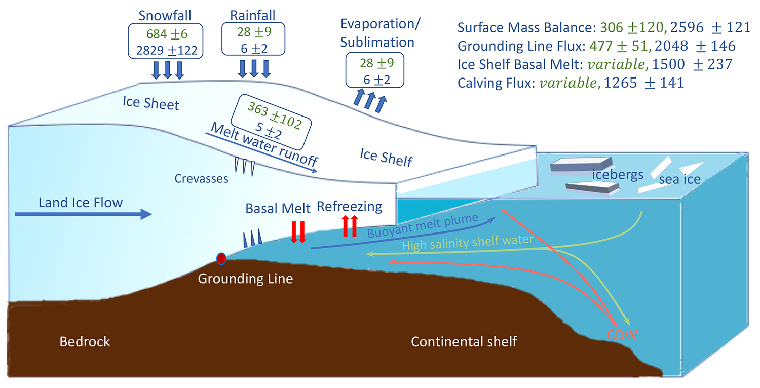
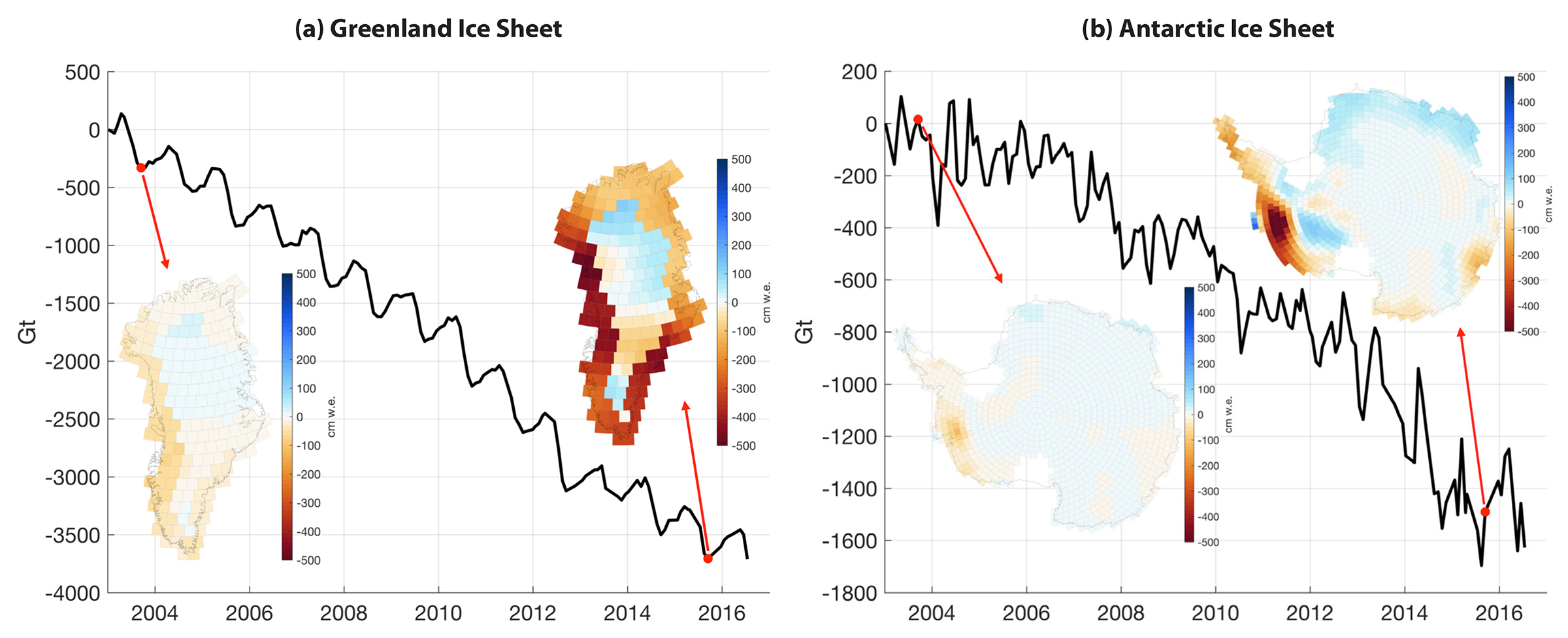
Ice sheets contain the largest reservoirs of freshwater on Earth, and the mass fluxes between ice sheets, atmosphere, and ocean are complex (Figure 1). Ice sheets gain mass due to snowfall and accretion beneath ice shelves, and lose mass via melting and iceberg calving (Cuffey and Paterson, 2010). Figure 2 shows the complexity of spatiotemporal mass changes that result from interannual variations in surface mass balance (SMB) and ice dynamics. Ice dynamics refers to changes in ice sheet flow, and is generally concentrated along outlet glaciers. In contrast, SMB changes occur across the entire ice sheet and arise from surface processes (evaporation, surface melt, and accumulation). Although surface melting and meltwater runoff are increasingly large components of the Greenland Ice Sheet surface mass balance, they are limited to the margins in Antarctica (Rignot et al., 2013; Enderlin et al., 2014; van den Broeke et al., 2016).

 

Figure 1. Schematic representation of ice sheet mass exchange with the atmosphere and ocean. Typical mass fluxes for the Antarctic (blue) and Greenland (green) Ice Sheets are in Gt yr–1 (360 Gt = 1 mm of sea level). Sub-shelf basal melt and calving flux for Greenland are uncertain and variable, hence excluded. Sources: van den Broeke et al. (2016), Rignot et al. (2013). > Full res figure

 

Figure 2. Mass change over the Greenland (a) and Antarctic (b) ice sheets as observed by NASA’s Gravity Recovery and Climate Experiment (GRACE). The time evolution of the mass loss (black) seen by GRACE is due to both dynamical mass loss and fluctuations in surface mass balance. The maps show changes from the start of the time series to the end of the melt seasons in 2003 and 2015, respectively. These reveal significant Greenland ice mass losses along the coast and moderate mass increases in the northern interior over the course of the GRACE mission, along with increasing significant mass loss over West Antarctica. Results shown are computed from the NASA GSFC mascons v2.4. Courtesy of Bryant Loomis, NASA Goddard Space Flight Center. > Full res figure

 

Three distinct remote-sensing techniques are currently used to study the mass change of ice sheets (Shepherd et al., 2012): (1) altimetry (based on ice sheet elevation changes), (2) gravimetry (based on gravity field changes), and (3) the input-output method (estimation of the difference between ice gain from accumulation and ice loss from surface runoff and ice discharge at the periphery). These methods resulted in a spread of ice sheet mass change estimates (−72 Gt yr^–1 to 684 Gt yr^–1) that motivated the Ice Sheet Mass Balance Intercomparison Experiment (IMBIE; Shepherd et al., 2012). IMBIE’s aim was to reconcile differences in satellite measurements of ice sheets mass balance from 1992 to 2011, and IMBIE2 extended this record to 2017 for Antarctica (Shepherd et al., 2018).

The Greenland Ice Sheet was in equilibrium with climate conditions in the early 1990s, and it therefore did not contribute significantly to sea level rise at that time. Its sea level contribution increased to 142 ± 49 Gt yr^–1 during 1992–2011, accelerating from 51 ± 65 Gt yr^–1 in 1992–2000 to 211 ± 37 Gt yr^–1 in 2000–2011 (Shepherd et al., 2012). The mass loss was equally split between increased ice discharge and greater surface meltwater runoff from 1996 to 2008; however, surface runoff changes increased to two-thirds of the mass loss in 2009–2012 (Enderlin et al., 2014). Although most outlet glaciers are thinning, at times there are episodes of thickening (Csatho et al., 2014). A similar story is revealed with ice velocity observations, with glaciers generally speeding up, but sometimes slowing down (Moon et al., 2012). Adjacent glaciers may evolve differently, as illustrated by Willis et al. (2018, in this issue) for Greenland’s Tracy and Heilprin Glaciers.

For the Antarctic Ice Sheet, the reconciled IMBIE2 mass losses were 109 ± 56 Gt yr^–1 for 1992–2017, with 76 ± 59 Gt yr^–1 during 1992–2011 and 219 ± 43 Gt yr^–1 between 2012 and 2017 (Shepherd et al., 2018). The Antarctic Peninsula was close to balance in the 1990s, but observations revealed increased dynamical mass loss following, for example, calving front retreat and disintegration of the Larsen B Ice Shelf in 2002 (Berthier et al., 2012). West Antarctica is the leading source of Antarctic mass loss throughout the IMBIE2 observational record (94 ± 27 Gt yr^–1), due to rapid acceleration, thinning, and grounding line retreat of the glaciers feeding the Amundsen Sea sector (Rignot et al., 2008; Shepherd et al., 2012). However, not all regions of West Antarctica are losing mass: the Kamb Ice Stream stagnated about 160 years ago (Retzlaff and Bentley, 1993) and is now gaining mass at a rate of 18 Gt yr^–1 (Rignot et al., 2008). Localized ice dynamical mass loss is also occurring in some parts of East Antarctica, such as the Totten and Cook Glaciers (Pritchard et al., 2009). However, these dynamic mass losses are smaller than the mass gain from snowfall over a large area (Figure 2), such that East Antarctica might have been gaining mass at an average rate of 5 ± 46 Gt yr^–1 over the 25-year observational record (Shepherd et al., 2018).

 

AN IMPROVED GENERATION OF MODELS

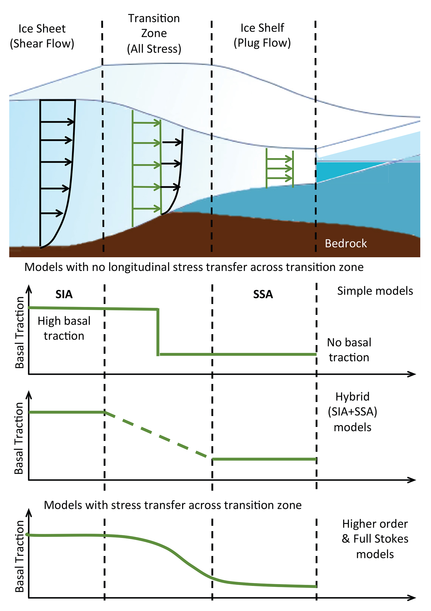
In its fourth assessment report (Meehl et al., 2007), the IPCC criticized the sea level projections from ISMs, as they could not replicate the observed rapid changes. As a result, several key features of ice flow models have improved greatly, including: (1) the approximation used for the stress balance equations (Figure 3), (2) the discretization of model domains (Figure 4), and (3) the representation of grounding lines and ice front migration. This section summarizes these improvements; for more details on recent ISM development, we refer readers to Goelzer et al. (2017) and Pattyn et al. (2017).

 

Figure 3. Illustration of a hierarchy of stress balance approximations available in ice sheet models. The Shallow Ice Approximation (SIA) assumes that flow is dominated by vertical shear stress, while the Shallow Shelf Approximation (SSA) assumes that flow is dominated by horizontal stress gradients. Hybrid models combine solutions from SIA and SSA. Higher order (HO) models include additional stresses to allow stress transmission across floating and grounded ice, while Full-Stokes (FS) models resolve all stresses. Adapted from Pattyn et al. (2006). > Full res figure

 

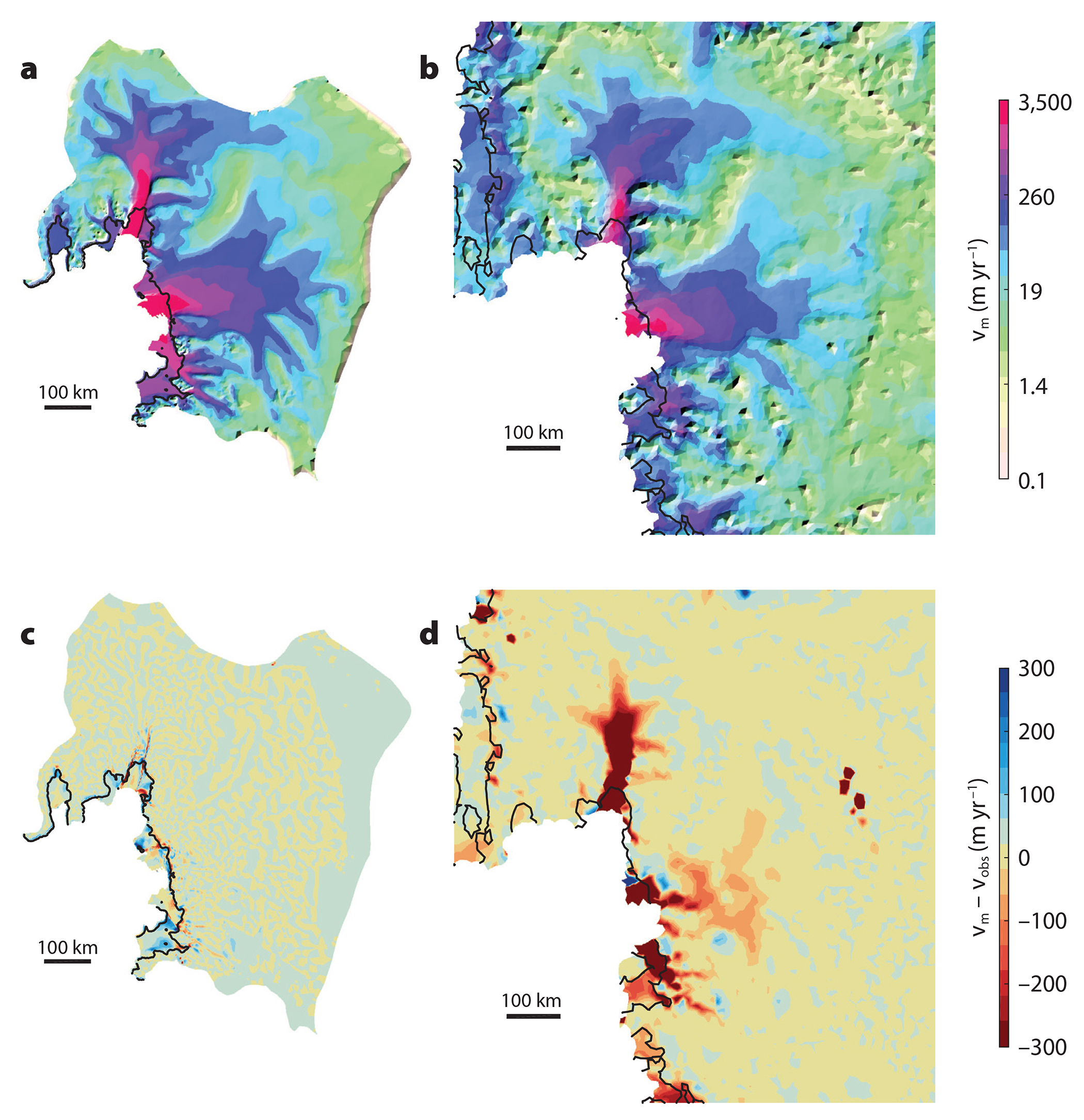
Figure 4. Impact of model resolution on models of the Amundsen Sea Sector. Modeled ice surface velocity after optimization (a,b) and difference between the modeled and observed velocity used in the optimization (c,d). Comparison of a regional model with a mesh resolution varying between 500 m and 5 km (a,c) and a continental scale Antarctic model with a 10 km resolution (b,d), obtained using the Ice Sheet System Model (Larour et al., 2012).  > Full res figure

 

To reproduce the rapid changes in the flow of the Antarctic and Greenland Ice Sheets, approximations of the Stokes equations that are valid in fast-flowing outlet glaciers, ice streams, and ice shelves were implemented. As Figure 3 shows, these new approximations replace the Shallow Ice Approximation (Hutter, 1982), which only represents vertical shear, and range from the Shelfy-Stream Approximation (MacAyeal, 1989) that captures the motion of ice shelves and fast-flowing ice streams to the complete Stokes equations that combine the momentum and incompressibility equations. To optimize the computational time, higher order models that neglect some components of the momentum balance equations, but that are valid in most regions (Pattyn, 2003; Schoof and Hindmarsh, 2010), and combinations thereof (Seroussi et al., 2012; Ahlkrona et al., 2016) were also developed. These improved stress balance approximations permit better simulation of rapidly changing glaciers (Morlighem et al., 2010).

Simultaneously, significant improvements were achieved in the discretization of ice flow domains. Thanks to the increased computational power and parallelization of ISMs (Larour et al., 2012), the typical grid resolution of continental-​scale models decreased from several tens or hundreds of kilometers to 10 km or less, improving the representation of tributary glaciers, shear margins, and critical areas, as well as the agreement with observations (see Figure 4). The introduction of a mesh with varying resolution (Morlighem et al., 2010) allowed models to combine fine resolution in critical areas with coarser resolutions in stagnant areas, and some models allow this refinement to evolve with time using adaptive remeshing techniques (Cornford et al., 2013). These refinements led to an almost doubling of grounding line retreat and to ice mass loss up to an order of magnitude higher (Cornford et al., 2013).

Accurate modeling of grounding line migration is critical, as this process is a major control on the stability of marine ice sheets and their mass loss (Durand et al., 2009). This field is another where substantial progress has been made: early models only included the grounded part of ice sheets, as ice shelf buttressing was thought not to influence the flow of grounded ice (Whillans and van der Veen, 1993). To capture the impact of changes in the ice shelves, Schoof (2007) proposed a grounding line flux parameterization that was implemented in several large-scale models (Pollard and Deconto, 2012). Most ISMs, however, determine grounding line positions directly, based on hydrostatic equilibrium. Refined grounding line position based on subgrid parameterizations (Pattyn et al., 2006; Seroussi et al., 2014) improved the ability of models to accurately simulate its position while limiting the need for high grid resolution. Models implementing the Stokes equations include a nonhydrostatic grounding line representation based on contact mechanics (Nowicki and Wingham, 2008; Durand et al., 2009). The Marine Ice Sheet Intercomparison Projects (MISMIP, Pattyn et al., 2012; MISMIP3D, Pattyn et al., 2013; MISMIP+, Asay-Davis et al., 2016) are advancing our ability to improve the representation of grounding line motion in numerical models, and to define minimum requirements to correctly include this process.

Modeling ice front evolution poses significant challenges both in terms of numerical implementation and understanding of calving. Numerical implementation of moving boundaries was performed in a number of models, either with subgrid parameterization (Albrecht et al., 2011) or level-set methods (conceptual frameworks for computing and analyzing the motion of an interface, here the ice front; Pralong and Funk, 2004; Bondzio et al., 2017). Such numerical schemes enable models to simulate the impact of ice front position on ice dynamics (Martin et al., 2011; Bondzio et al., 2017). The physical processes driving calving, however, remain poorly understood, as discussed in a recent review of calving (Benn et al., 2017).

Our understanding of ice sheets is constantly evolving with the discovery of new processes such as ice shelf damage (Borstad et al., 2016), subglacial hydrology (Creyts and Schoof, 2009), and cryo-hydrologic warming (Phillips et al., 2010), as well as with knowledge of the nature of the underlying bed (Christianson et al., 2013) and the evolution in properties of basal conditions (Gillet-Chaulet et al., 2016). Such processes and understanding are starting to be implemented in regional ISMs and should be more systematically included in future simulations.

 

LINKING MODELS AND OBSERVATIONS

In the past decade, we witnessed a shift from a world with very limited modern observations to an era with abundant high temporal and spatial resolution data. Newly acquired data and improved models influence each other in terms of requirements, areas studied, and limitations. The launch of several satellite and airborne missions made available a wide range of large-scale observations that are being used to better initialize, constrain, and validate ISMs. Prior to the first complete maps of ice surface velocity (published fewer than 10 years ago; Joughin et al., 2010; Rignot et al., 2011), it was impossible to compare one of the main model diagnostics, ice velocity, with large-scale observations. The improved description of geometry was directly included in ISMs to define their initial states (Bamber et al., 2013; Fretwell et al., 2013). The opportunities offered by these new observations, however, go well beyond their simple use as model inputs. Using data assimilation methods, modelers were able to infer ice properties that cannot be directly observed, such as basal conditions that are buried under kilometers of ice, or rigidity of ice shelves (MacAyeal, 1992; Joughin et al., 2001; Goelzer et al., 2018).

The systematic use of observations went even further: ISMs started to combine observations with model physics to evaluate ice parameters in areas where observations are lacking. Large errors resulting from a limited coverage of ice geometry made these observational data sets difficult to use in models (Seroussi et al., 2011). As a result, mass conservation algorithms that estimate ice thickness from ice surface velocities, existing (but sparse) thickness measurements, surface mass balance, and surface elevation changes were developed (Morlighem et al., 2011). The maps created provide additional details about bedrock topography and show that Greenland fjords extend deeper and further inland than previously thought, making them more vulnerable to ocean warming (Morlighem et al., 2014).

All these improvements greatly enhanced the models’ ability to reproduce current ice sheet characteristics, especially for outlet glaciers (Figure 4), where changes are the most significant (Seroussi et al., 2017). Because models are now able to replicate observed changes over the past couple of decades, hindcasting is becoming possible (Aschwanden et al., 2013). Observations are also used to calibrate projections of ice sheet changes over the coming centuries in ensemble runs, such that simulations with the best agreement to the past evolution are given a higher weight in the projections (Ritz et al., 2015). However, accurately simulating the future evolution of ice sheets remains very challenging, as models’ initial states (Goelzer et al., 2018) and external forcings need to be better constrained.

 

SEA LEVEL PROJECTIONS: BEYOND AN ICE SHEET MODEL PROBLEM

Credible ice sheet projections rely not only on ISMs, but also on knowledge of boundary conditions and future climatic forcing. Thus, reducing the uncertainty in future sea level rise resulting from ice sheet melting requires advances in and tighter collaborations with other disciplines. In an attempt to bridge the gap between the ice sheet and climate communities, the Coupled Model Intercomparison Project Phase 6 (CMIP6) endorsed the Ice Sheet Model Intercomparison for CMIP6 (ISMIP6; Nowicki et al., 2016; Eyring et al., 2016). ISMIP6 experimental protocol combines simulations of stand-alone ISMs driven offline from forcings generated from coupled atmosphere-ocean climate models and simulations generated from coupled ice sheet-atmosphere-ocean models.

Much progress has been made in recent years, with global climate models beginning to generate SMBs that compare well with regional climate models (Vizcaino et al., 2013; Lenaerts et al., 2016). These simulations, in which ice sheet extent and elevation are fixed in the climate model, focus on improving surface processes and polar climate over the ice sheets. Nonetheless, challenges in representing ice-atmosphere interactions and SMB remain, and we refer the reader to recent reviews in this field (Favier et al., 2017, van den Broeke et al., 2017). Simulations in which ice sheets fully interact with the atmosphere in climate models show promising results and demonstrate the importance of ice sheets as an interactive component of climate models. For example, allowing for elevation-SMB feedback increases the surface runoff at lower elevations and thus the contribution of the Greenland Ice Sheet to sea level rise (Vizcaino et al., 2015).

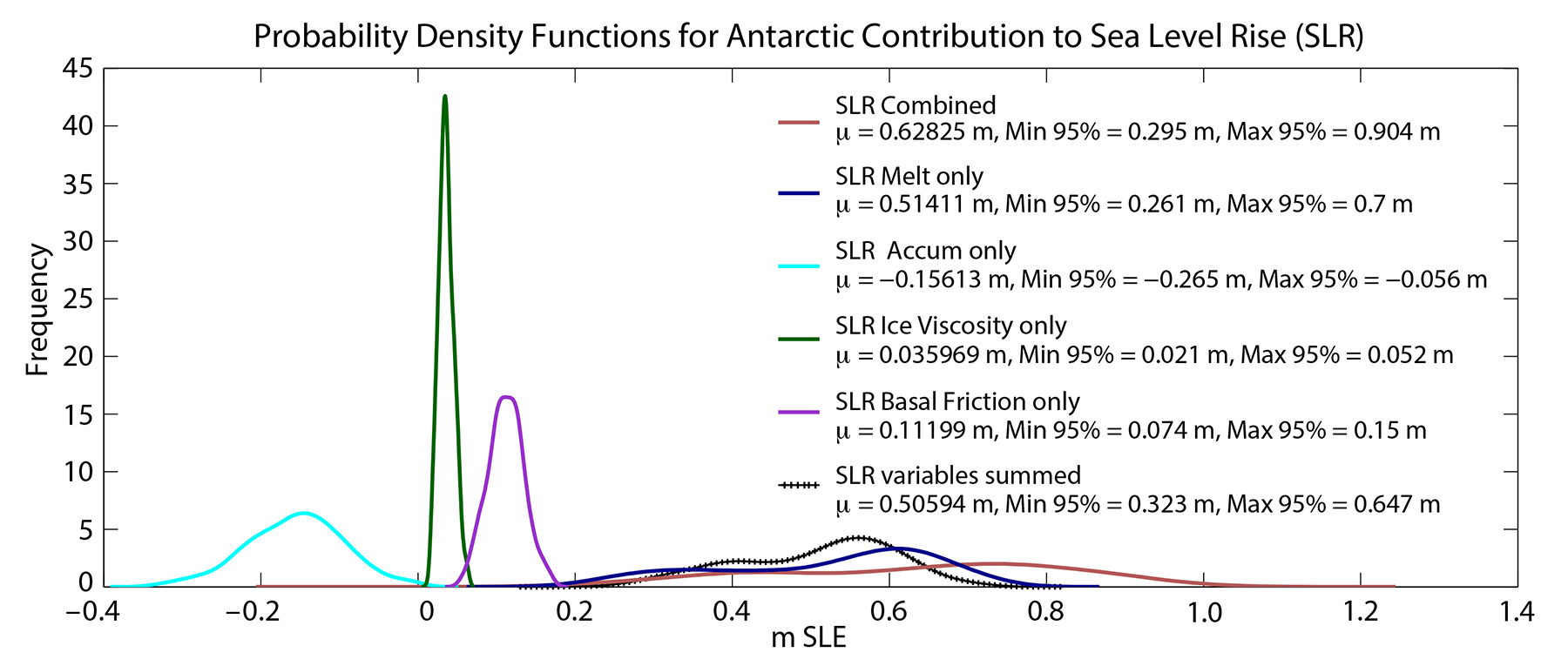
Representing ice-ocean interactions accurately in ISMs is critical, as changes in oceanic conditions have the potential to impact ice sheet dynamics on interannual (Steig et al., 2012; Greene et al., 2017) to centennial (Rahmstorf, 2002; Alley et al., 2005) timescales through evolving melt rates under ice shelves and along calving fronts. An exploration of the sensitivity of Antarctica’s contribution to sea level rise in response to uncertainties in external forcing, boundary conditions, and input parameters shows that uncertainties in ice shelf melt rates dominate the continent’s sea level contribution and its uncertainty over the next 100 years (Figure 5 and Schlegel et al., 2018). Studies on fast-flowing glaciers in the Amundsen Sea sector came to a similar conclusion regarding the dominant role ocean-induced melting plays in controlling ice dynamics, as higher melt rates reduce ice shelf buttressing and accelerate grounding line retreats (Favier et al., 2014; Seroussi et al., 2017). An accurate representation of oceanic forcing is, however, challenging because of the technical difficulty of coupling ice sheet and ocean models with a dynamic boundary, the limited understanding of physical processes governing ice-ocean interactions, and the limited number of oceanic observations in ice shelf cavities, including observations of oceanic properties and also bathymetry and bedrock under both floating and grounded ice (Colloni et al., 2018).

 

Figure 5. Probability distributions of the Antarctic Ice Sheet contribution to sea level rise in 2100, based on 800 simulation ensembles sampled within a given uniform distribution of error. Solid lines show the impact of uncertainties in the ocean-induced melting rate (dark blue), surface mass balance (light blue), ice viscosity (green), basal friction (purple), and the combination of these four parameters (red). The black crossed line shows the sum of the four independent ensembles. The legend indicates the mean, lower 95%, and upper 95% distribution values for each ensemble. Adapted from Schlegel et al. (2018). > Full res figure

 

Understanding the feedback between ice sheets and large-scale ocean circulation, as well as the impacts of their variability, requires models to interactively couple these two systems (Fyke et al., 2018). The first studies relying on coupled ice-ocean models show that simulations performed with parameterizations of ice shelf melt tend to overestimate glacier changes and mass loss compared to simulations performed with coupled ice-ocean models (De Rydt and Gudmundsson, 2016; Seroussi et al., 2017). The coupled models agree better with observations of real glacier changes and grounding line retreat, in particular (Seroussi et al., 2017). Developing Earth system models that couple the atmosphere, ocean, land, ice, and biosphere would be the best approach to accurately simulating these interactions, but these models have coarse resolutions (~ 50–100 km in the polar regions) that limit their accuracy in critical areas such as narrow glacier fjords around Greenland, and no model of the CMIP5 ensemble resolved the ocean circulation in ice shelf cavities (Flato et al., 2013; Straneo et al., 2013). Furthermore, these models do not include dynamic boundaries for their different components, which are critical for representing ice shelf cavity evolution or ice front retreat. The only solution so far for including large-scale ocean changes in ocean forcings for the ice sheets is to translate these changes into parameterizations based on oceanic conditions and ice sheet configurations (Asay-Davis et al., 2017), but neglecting the feedbacks between these systems.

A challenge for any simulation of sea level change from ISMs is obtaining an accurate initial state. Two distinct methods were traditionally used for stand-alone ISMs, spin-ups and data assimilation (Nowicki et al., 2013), but we are now seeing approaches that combine these two methods (Goelzer et al., 2018). Spin-up methods that permit ISMs to be in equilibrium with climatic forcing or to retain some transient memory of previous climatic changes are currently available for the Greenland and the Antarctic Ice Sheets. However, spin-ups often result in an ice sheet geometry that differs from that of the present day (Nowicki et al., 2013; Goelzer et al., 2018). Data assimilation in most ISMs relies on assimilating snapshots of observations and assumes a steady state for the present-day ice sheet. A path forward for obtaining a time-​evolving state would be to combine existing observational time series into a reanalysis, similar to what is being done in physical oceanography to provide the best possible ocean state estimates (Menemenlis et al., 2008). A few studies have been performed by assimilating time series of observations (Goldberg and Heimbach, 2013; Larour et al., 2014). They show that forecasting is much improved when models are initialized not with a snapshot of observations but with longer time series. Many ISMs are working toward this goal, and we can expect to see a lot of progress along this line over the coming decade. Another emerging area of research is how to best initialize ISMs within fully coupled Earth system models (Nowicki et al., 2016; Fyke et al., 2018).

 

CONCLUSIONS

The collection of annual to weekly observations of ice sheet surface velocity, surface elevation, and mass change (Mouginot et al., 2014; Mililo et al., 2017; Csatho et al., 2014) marks the start of a new era for ice flow modeling. We recently switched from a no-data world to one with an abundance of observations, but modelers are challenged when these observations do not agree, as illustrated by the IMBIE efforts and the need to reconcile observations of ice sheet mass change. We are also reaching an era when ISMs can provide insight on observations (type, scope, location, and resolution) that are most needed for improving projections. An example is the sparsity of bedrock topography data under ice streams (in particular, in the vicinity of grounding lines) and beneath ice shelves. There is an urgent need for observation-based scientists and modelers to increase their collaborations in order to fully understand the drivers of observed changes over the polar regions and to analyze which processes, interactions, and feedback are crucial and which ones can be ignored in models.

What can be expected in terms of projections of future sea level? Considering the rapid ISM developments that have occurred over the last decades, a major challenge is obtaining realistic atmospheric and oceanic forcing for ice sheets. Thus, there is an urgent need for improved polar climate representation from Earth system models, which is also necessary for the coupling of ice sheet-climate models. The inclusion of ISMs in Earth system models has resulted in a focus on improving the SMB generated by these models and a better understanding of ice-atmosphere interactions. Modeling ice-ocean interactions and coupling ISMs to ocean models remain extremely challenging, in part due to the difficulties in collecting observations beneath the ice shelves, our poor knowledge of the bathymetry beneath ice shelf cavities, and the numerical challenge of creating ocean models that have the capability to adjust their domains as the ice sheet evolves. Reducing uncertainties in sea level contributions from ice sheets is therefore becoming a problem that is no longer simply an ice sheet modeling problem.

Nowicki, S., and H. Seroussi. 2018. Projections of future sea level contributions from the Greenland and Antarctic Ice Sheets: Challenges beyond dynamical ice sheet modeling. Oceanography 31(2):109–117, https://doi.org/10.5670/oceanog.2018.216.

Ahlkrona, J., P. Lotstedt, N. Kirchner, and T. Zwinger. 2016. Dynamically coupling the non-linear Stokes equations with the shallow ice approximation in glaciology: Description and first applications of the ISCAL method. Journal of Computational Physics 308, https://doi.org/10.1016/​j.jcp.2015.​12.025.

Albrecht, T., M. Martin, M. Haselo, R. Winkelmann, and A. Levermann. 2011. Parameterization for subgrid-scale motion of ice-shelf calving fronts. Cryosphere 5(1):35–44, https://doi.org/10.5194/tc-5-35-2011.

Alley, R., P. Clark, P. Huybrechts, and I. Joughin. 2005. Ice-sheet and sea-level changes. Science 310(5747):456–460, https://doi.org/10.1126/science.1114613.

Asay-Davis, X., S.L. Cornford, G. Durand, B.K. Galton-Fenzi, R.M. Gladstone, G.H. Gudmundsson, T. Hattermann, D.M. Holland, D. Holland, P.R. Holland, and others. 2016. Experimental design for three interrelated Marine Ice-Sheet and Ocean Model Intercomparison Projects: MISMIP v.3 (MISMIP+), ISOMIP v.2 (ISOMIP+) and MISOMIP v.1 (MISOMIP1). Geoscientific Model Development 9:2,471–2,497, https://doi.org/​10.5194/​gmd-9-2471-2016.

Asay-Davis, X.S., N.C. Jourdain, and Y. Nakayama. 2017. Developments in simulating and parameterizing interactions between the Southern Ocean and the Antarctic ice sheet. Current Climate Change Reports 3(4):316–329, https://doi.org/10.1007/s40641-017-0071-0.

Aschwanden, A., G. Adakgeirsdottir, and C. Khroulev. 2013. Hindcasting to measure ice sheet model sensitivity to initial states. Cryosphere 7(4):1,083–1,093, https://doi.org/10.5194/tc-7-1083-2013.

Bamber, J.L., J.A. Griggs, R.T.W.L. Hurkmans, J.A. Dowdeswell, S.P. Gogineni, I. Howat, J. Mouginot, J. Paden, S. Palmer, E. Rignot, and D. Steinhage. 2013. A new bed elevation dataset for Greenland. Cryosphere 7:499–510, https://doi.org/​10.5194/​tc-7-499-2013.

Benn, D.I., T. Cowton, J. Todd, and A. Luckman. 2017. Glacier calving in Greenland. Current Climate Change Reports 3:282–290, https://doi.org/​10.1007/s40641-017-0070-1.

Berthier, E., T. Scambos, and C. Shuman. 2012. Mass loss of Larsen B tributary glaciers (Antarctic Peninsula) unabated since 2002. Geophysical Research Letters 39, L13501, https://doi.org/​10.1029/2012GL051755.

Bondzio, J.H., M. Morlighem, H. Seroussi, T. Kleiner, M. Rückamp, J. Mouginot, T. Moon, E.Y. Larour, and A. Humbert. 2017. The mechanisms behind Jakobshavn Isbrea’s acceleration and mass loss: A 3-D thermomechanical model study. Geophysical Research Letters 44:6,252–6,260, https://doi.org/​10.1002/​2017GL073309.

Borstad, C., A. Khazendar, B. Scheuchl, M. Morlighem, E. Larour, and E. Rignot. 2016. A constitutive framework for predicting weakening and reduced buttressing of ice-shelves based on observations of the progressive deterioration of the remnant Larsen B ice shelf. Geophysical Research Letters 43(5):2,027–2,035, https://doi.org/​10.1002/2015GL067365.

Christianson, K., B.R. Parizek, R.B. Alley, H.W. Horgan, R.W. Jacobel, S. Anandakrishnan, B.A. Keisling, B.D. Craig, and A. Muto. 2013. Ice sheet grounding zone stabilization due to till compaction. Geophysical Research Letters 40(20):5,406–5,411, https://doi.org/10.1002/2013gl057447.

Church, J.A., P.U. Clark, A. Cazenave, J.M. Gregory, S. Jevrejeva, A. Levermann, M.A. Merrifield, G.A. Milne, R.S. Nerem, P.D. Nunn, and others. 2013. Sea level change. Pp. 1,137–1,216 in Climate Change 2013: The Physical Science Basis. Contribution of Working Group I to the Fifth Assessment Report of the Intergovernmental Panel on Climate Change. T.F. Stocker, D. Qin, G.-K. Plattner, M. Tignor, S.K. Allen, J. Boschung, A. Nauels, Y. Xia, V. Bex, and P.M. Midgley, eds, Cambridge University Press, Cambridge, UK, and New York, NY, USA, https://doi.org/10.1017/CBO9781107415324.026.

Colloni, F., L. De Santis, C.S. Siddoway, A. Bergamasco, N.R. Golledge, G. Lohmann, S. Passchier, and M.J. Siegert. 2018. Spatio-temporal variability of processes across Antarctic ice-bed-ocean interfaces. Nature Communications 9(2289):2,041–1,723, https://doi.org/​10.1038/s41467-018-04583-0.

Cornford, S.L., D.F. Martin, D.T. Graves, D.F. Ranken, A.M. Le Brocq, R.M. Gladstone, A.J. Payne, E.G. Ng, and W.H. Lipscomb. 2103. Adaptive mesh, finite volume modeling of marine ice-sheets. Journal of Computational Physics 232(1):529–549, https://doi.org/​10.1016/j.jcp.2012.08.037.

Creyts, T.T., and C.G. Schoof. 2009. Drainage through subglacial water sheets. Journal of Geophysical Research 114:1–18, https://doi.org/​10.1029/2008JF001215.

Csatho, B.M., A.F. Schenk, C.J. van der Veen, G. Babonis, K. Duncan, S. Rezvanbehbahani, M.R. van den Broeke, S.B. Simonsen, S. Nagarajan, and J.H. van Angelen. 2014. Laser altimetry reveals complex pattern of Greenland ice sheet dynamics. Proceedings of the National Academy of Sciences of the United States of America 111(52):18,478–18,483, https://doi.org/​10.1073/pnas.1411680112.

Cuffey, K.M., and W.S.B Paterson. 2010. The Physics of Glaciers, 4th ed. Academic Press Amsterdam, 704 pp.

DeConto, R., and D. Pollard. 2016. Contribution of Antarctica to past and future sea-level rise. Nature 531:591–597, https://doi.org/10.1038/nature17145.

De Rydt, J., and G.H. Gudmundsson. 2016. Coupled ice shelf-ocean modeling and complex grounding line retreat from a seabed ridge. Journal of Geophysical Research 121:865­–880, https://doi.org/​10.1002/​2015JF003791.

Durand, G., O. Gagliardini, B. de Fleurian, T. Zwinger, and E. Le Meur. 2009. Marine ice sheet dynamics: Hysteresis and neutral equilibrium. Journal of Geophysical Research 114, F03009, https://doi.org/​10.1029/2008JF001170.

Dutton, A., A.E. Carlson, A.J. Long, G.A. Milne, P.U. Clark, R. DeConto, B.P. Horton, S. Rahmstorf, and M.E. Raymo. 2015. Sea-level rise due to polar ice-sheet mass loss during past warm periods. Science 349(6244):aaa4019, https://doi.org/10.1126/science.aaa4019.

Enderlin, E.M., I.M. Howat, S. Jeong, M.-J. Noh, J.H. van Angelen, and M.R. van den Broeke. 2014. An improved mass budget for the Greenland ice sheet. Geophysical Research Letters 41(3):866–872, https://doi.org/​10.1002/​2013GL059010.

Eyring, V., S. Bony, G.A. Meehl, C.A. Senior, B. Stevens, R.J. Stouffer, and K.E. Taylor. 2016. Overview of the coupled model intercomparison project phase 6 (CMIP6) experimental design and organization. Geoscientific Model Development 9(5):1,937–1,958, https://doi.org/​10.5194/gmd-9-1937-2016.

Favier, L., G. Durand, S.L. Conford. G.H. Gudmundsson, O. Gagliardini, F. Gillet-Chaulet, T. Zwinger, A.J. Payne, and A.M. Le Brocq. 2014. Retreat of Pine Island Glacier controlled by marine ice-sheet instability. Nature Climate Change 4:117–121, https://doi.org/10.1038/NCLIMATE2094.

Favier, V., G. Krinner, C. Amory, H. Gallée, J. Beaumet, and C. Agosta. 2017. Antarctica-regional climate and surface mass budget. Current Climate Change Reports 3(4):303–315, https://doi.org/10.1007/s40641-017-0072-z.

Flato, G., J. Marotzke, B. Abiodun, P. Braconnot, S.C. Chou, W. Collins, P. Cox, F. Driouech, S. Emori, V. Eyring, and others. 2013. Evaluation of climate models. Pp. 741–866 in Climate Change 2013: The Physical Science Basis. Contribution of Working Group I to the Fifth Assessment Report of the Intergovernmental Panel on Climate Change. T.F. Stocker, D. Qin, G.-K. Plattner, M. Tignor, S.K. Allen, J. Boschung, A. Nauels, Y. Xia, V. Bex, and P.M. Midgley, eds, Cambridge University Press, Cambridge, UK, and New York, NY, USA, https://doi.org/​10.1017/​CBO9781107415324.020.

Fretwell, P., H.D. Pritchard, D.G. Vaughan, J.L. Bamber, N.E. Barrand, R. Bell, C. Bianchi, R.G. Bingham, D.D. Blankenship, G. Casassa, and others. 2013. Bedmap2: Improved ice bed, surface and thickness datasets for Antarctica. Cryosphere 7(1):375–393, https://doi.org/10.5194/tc-7-375-2013.

Fyke, J., O. Sergienko, M. Lofverstrom, S. Price, and J. Lenaerts. 2018. An overview of interactions and feedbacks between ice sheets and the Earth system. Reviews of Geophysics 56, https://doi.org/​10.1029/2018RG000600.

Gillet-Chaulet, F., G. Durand, O. Gagliardini, C. Mosbeux, J. Mouginot, F. Rémy, and C. Ritz. 2016. Assimilation of surface velocities acquired between 1996 and 2010 to constrain the form of the basal friction law under Pine Island Glacier. Geophysical Research Letters 43:10,311–10,321, https://doi.org/10.1002/2016GL069937.

Goelzer, H., S. Nowicki, T. Edwards, M. Beckley, A. Abe-Ouchi, A. Aschwanden, R. Calov, O. Gagliardini, F. Gillet-Chaulet, N.R. Golledge, and others. 2018. Design and results of the ice sheet model initialisation experiments initMIP-Greenland: An ISMIP6 intercomparison. Cryosphere 12:1,433-1,460, https://doi.org/10.5194/tc-2017-129.

Goelzer, H., A. Robinson, H. Seroussi, and R.S.W. van de Wal. 2017. Recent progress in Greenland ice sheet modeling. Current Climate Change Reports 3(4):291–302, https://doi.org/10.1007/s40641-017-0073-y.

Goldberg, D.N., and P. Heimbach. 2013. Parameter and state estimation with a time-​dependent adjoint marine ice sheet model. Cryosphere 17:1,659–1,678, https://doi.org/10.5194/tc-7-1659-2013.

Greene, C.A., D.D. Blankenship, D.E. Gwyther, A. Silvano, and E. van Wijk. 2017. Wind causes Totten Ice Shelf melt and acceleration. Science Advances 3(11):e1701681, https://doi.org/10.1126/sciadv.1701681.

Hutter, K. 1982. Dynamics of glaciers and large ice masses. Annual Review of Fluid Mechanics 14:87–130, https://doi.org/10.1146/annurev.fl.14.010182.000511.

Jacobs, S.S., A. Jenkins, C.F. Giulivi, and P. Dutrieux. 2011. Stronger ocean circulation and increased melting under Pine Island Glacier ice shelf. Nature Geosciences 4(8):519–523, https://doi.org/10.1038/NGEO1188.

Joughin, I., M. Fahnestock, D. MacAyeal, J. Bamber, and P. Gogineni. 2001. Observation and analysis of ice flow in the large Greenland ice stream. Journal of Geophysical Research 106(D24):34,021–34,034, https://doi.org/10.1029/2001JD900087.

Joughin, I., B. Smith, I. Howat, T. Scambos, and T. Moon. 2010. Greenland flow variability from ice-sheet-wide velocity mapping. Journal of Glaciology 56:416–430, https://doi.org/​10.3189/​002214310792447734.

Larour, E., H. Seroussi, M. Morlighem, and E. Rignot. 2012. Continental scale, high order, high spatial resolution, ice sheet modeling using the Ice Sheet System Model (ISSM). Journal of Geophysical Research 117, F01022, https://doi.org/​10.1029/2011JF002140.

Larour, E., J. Utke, B. Csatho, A. Schenk, H. Seroussi, M. Morlighem, E. Rignot, N. Schlegel, and A. Khazendar. 2014. Inferred basal friction and surface mass balance of the Northeast Greenland Ice Stream using data assimilation of ICESat (Ice Cloud and land Elevation Satellite) surface altimetry and ISSM (Ice Sheet System Model). Cryosphere 8(6):2,335–2,351, https://doi.org/​10.5194/tc-8-2335-2014.

Lenaerts, J., M. Vizcaino, J. Fyke, L. van Kampenhout, and M. van den Broeke. 2016. Present-day and future Antarctic ice sheet climate and surface mass balance in the Community Earth System Model. Climate Dynamics 5-6:1,367–1,381, https://doi.org/​10.1007/s00382-015-2907-4.

MacAyeal, D.R. 1989. Large-scale ice flow over a viscous basal sediment: Theory and application to Ice Stream B, Antarctica. Journal of Geophysical Research 94(B4):4,071–4,087, https://doi.org/​10.1029/​JB094iB04p04071.

MacAyeal, D.R. 1992. The basal stress distribution of Ice Stream E, Antarctica, inferred by control methods. Journal of Geophysical Research 97(B1):595–603, https://doi.org/​10.1029/91JB02454.

Martin, M.A., R. Winkelmann, M. Haseloff, T. Albrecht, E. Bueler, C. Khroulev, and A. Levermann. 2011. The Potsdam Parallel Ice Sheet Model (PISM-PIK): Part 2. Dynamic equilibrium simulation of the Antarctic ice sheet. Cryosphere 5(3):727–740, https://doi.org/10.5194/tc-5-727-2011.

Meehl, G.A., T.F. Stocker, W.D. Collins, P. Friedlingstein, A.T. Gaye, J.M. Gregory, A. Kitoh, R. Knutti, J.M. Murphy, A. Noda, and others. 2007. Global climate projections. Pp. 747–845 in Climate Change 2007: The Physical Science Basis. Contribution of Working Group I to the Fourth Assessment Report of the Intergovernmental Panel on Climate Change. S. Solomon, D. Qin, M. Manning, Z. Chen, M. Marquis, K.B. Averyt, M. Tignor, and H.L. Miller, eds, Cambridge University Press, Cambridge, UK, and New York, NY, USA.

Menemenlis, D., J.-M. Campin, P. Heimbach, C. Hill, T. Lee, A. Nguyen, M. Schodlok, and H. Zhang. 2008. ECCO 2: High resolution global ocean and sea ice data synthesis. Mercator Ocean Quarternary Newsletter 31:13–21.

Milillo, P., E. Rignot, J. Mouginot, B. Scheuchl, M. Morlighem, X. Li, and J.T. Salzer. 2017. On the short-term grounding zone dynamics of Pine Island glacier, West Antarctica, observed with COSMO-SkyMed interferometric data. Geophysical Research Letters 44:10,436–10,444, https://doi.org/​10.1002/2017GL074320.

Moon, T., I. Joughin, B. Smith, and I. Howat. 2012. 21st-century evolution of Greenland outlet glacier velocities. Science 336(6081):576–578, https://doi.org/​10.1126/​science.1219985.

Morlighem, M., E. Rignot, J. Mouginot, H. Seroussi, and E. Larour. 2014. High-resolution ice thickness mapping in South Greenland. Annals of Glaciology 55(67):64–70, https://doi.org/​10.3189/​2014AoG67A088.

Morlighem, M., E. Rignot, H. Seroussi, E. Larour, H.B. Dhia, and D. Aubry. 2010. Spatial patterns of basal drag inferred using control methods from a full-Stokes and simpler models for Pine Island Glacier, West Antarctica. Geophysical Research Letters 37, L14502, https://doi.org/​10.1029/​2010GL043853.

Morlighem, M., E. Rignot, H. Seroussi, E. Larour, H.B. Dhia, and D. Aubry. 2011. A mass conservation approach for mapping glacier ice thickness. Geophysical Research Letters 38, L19503, https://doi.org/​10.1029/2011GL048659.

Mouginot, J., E. Rignot, and B. Scheuchl. 2014. Sustained increase in ice discharge from the Amundsen Sea embayment, West Antarctica, from 1973 to 2013. Geophysical Research Letters 41:1–9, https://doi.org/10.1002/2013GL059069.

Nowicki, S., R.A. Bindschadler, A. Abe-Ouchi, A. Aschwanden, E. Bueier, H. Choi, J. Fastook, G. Granzow, R. Greve, G. Gutowski, and others. 2013. Insights into spatial sensitivities of ice mass response to environmental change from the SeaRISE ice sheet modeling project I: Antarctica. Journal of Geophysical Research 118:1,002–1,024, https://doi.org/10.1002/jgrf.20081.

Nowicki, S.M.J., A. Payne, E. Larour, H. Seroussi, H. Goelzer, W. Lipscomb, J. Gregory, A. Abe-Ouchi, and A. Shepherd. 2016. Ice Sheet Model Intercomparison Project (ISMIP6) contribution to CMIP6. Geoscientific Model Development 9:4,521–4,545, https://doi.org/​10.5194/gmd-9-4521-2016.

Nowicki, S., and D.J. Wingham. 2008. Conditions for a steady ice sheet-ice shelf junction. Earth and Planetary Science Letters 265(1-2):246–255, https://doi.org/10.1016/j.epsl.2007.10.018.

Padman, L., M.R. Siegert, and H.A. Fricker. 2018. Ocean tide influences on the Antarctic and Greenland ice sheets. Reviews of Geophysics 56, https://doi.org/10.1002/2016RG000546.

Pattyn, F., 2003. A new three-dimensional higher-​order thermomechanical ice sheet model: Basic sensitivity, ice stream development, and ice flow across subglacial lakes. Journal of Geophysical Research 108(B8), https://doi.org/​10.1029/2002JB002329.

Pattyn, F., L. Favier, S. Sun, and G. Durand. 2017. Progress in numerical modeling of Antarctic ice-sheet dynamics. Current Climate Change Reports 3(4):174–184, https://doi.org/10.1007/s40641-017-0069-7.

Pattyn, F., A. Huyghe, S. De Brabander, and B. De Smedt. 2006. Role of transition zones in marine ice sheet dynamics. Journal of Geophysical Research 111(F2):1–10, https://doi.org/​10.1029/2005JF000394.

Pattyn, F., L. Perichon, G. Durand, and L. Favier. 2013. Grounding-line migration in plan-view marine ice-sheet models: Results of the ice2sea MISMIP3d intercomparison. Journal of Glaciology 59(215):410–422, https://doi.org/​10.3189/2013JoG12J129.

Pattyn, F., C. Schoof, L. Perichon, R.C.A. Hindmarsh, E. Bueler, B. de Fleurian, G. Durand, O. Gagliardini, R. Gladstone, D. Goldberg, and others. 2012. Results of the Marine Ice Sheet Model Intercomparison Project, MISMIP. Cryosphere 6(3):573–588, https://doi.org/10.5194/tc-6-573-2012.

Phillips, T., H. Rajaram, and K. Steffen. 2010. Cryo-hydrologic warming: A potential mechanism for rapid thermal response of ice sheets. Geophysical Research Letters 7:1–5, https://doi.org/​10.1029/​2010GL044397.

Pollard, D., and R.M. DeConto. 2012. A simple inverse method for the distribution of basal sliding coefficients under ice sheets, applied to Antarctica. Cryosphere 6(5):953–971, https://doi.org/10.5194/tc-6-953-2012.

Pralong, A., and M. Funk. 2004. A level-set method for modeling the evolution of glacier geometry. Journal of Glaciology 50(171):485–491, https://doi.org/​10.3189/​172756504781829774.

Pritchard, H., R. Arthern, D. Vaughan, and L. Edwards. 2009. Extensive dynamic thinning on the margins of the Greenland and Antarctic ice sheets. Nature 461:971–975, https://doi.org/10.1038/nature08471.

Rahmstorf, S. 2002. Ocean circulation and climate during the past 120,000 years. Nature 419:207–214, https://doi.org/10.1038/nature01090.

Retzlaff, R., and C. Bentley. 1993. Timing of stagnation of Ice Stream C, West Antarctica, from short-pulse radar studies of buried surface crevasses. Journal of Glaciology 39(133):553–561, https://doi.org/​10.3189/​S0022143000016440.

Rignot, E. 1998. Fast recession of a West Antarctic glacier. Science 281(5376):549–551, https://doi.org/​10.1126/science.281.5376.549.

Rignot, E., J.L. Bamber. M.R. van den Broeke, C. Davis, Y. Li, W.J. van de Berg, and E. van Meijgaard. 2008. Recent Antarctic ice mass loss from radar interferometry and regional climate modeling. Nature Geoscience 1(2):106–110, https://doi.org/10.1038/ngeo102.

Rignot, E., S. Jacobs, J. Mouginot, and B. Scheuchl. 2013. Ice-shelf melting around Antarctica. Science 341(6143):266–270, https://doi.org/10.1126/science.1235798.

Rignot, E., I. Velicogna, M. van den Broeke, A. Monaghan, and J. Lenaerts. 2011. Acceleration of the contribution of the Greenland and Antarctic ice sheets to sea-level rise. Geophysical Research Letters 38:1–5, https://doi.org/​10.1029/​2011GL046583.

Ritz, C., T.L. Edwards, G. Durand, A.J. Payne, V. Peyaud, and R.C.A. Hindmarsh. 2015. Potential sea-level rise from Antarctic ice-sheet instability constrained by observations. Nature 528(7580):1150118, https://doi.org/10.1038/nature16147.

Schlegel, N., H. Seroussi, M.P. Schodlok, E.Y. Larour, C. Boening, D. Limonadi, M.M. Watkins, M. Morlighem, and M.R. van den Broeke. 2018. Exploration of the Antarctic ice-sheet 100-year contribution to sea level rise and associated model uncertainties using the ISSM framework. The Cryosphere Discussions, https://doi.org/​10.5194/​tc-2018-105.

Schoof, C. 2007. Ice sheet grounding line dynamics: Steady states, stability, and hysteresis. Journal of Geophysical Research 112, F03S28, https://doi.org/​10.1029/​2006JF000664.

Schoof, C., and R.C.A. Hindmarsh, 2010. Thin-film flows with wall slip: An asymptotic analysis of higher order glacier flow models. Quarternary Journal of Mechanics and Applied Mathematics 63:73–114, https://doi.org/10.1093/qjmam/hbp025.

Seroussi, H., H.B. Dhia, M. Morlighem, E. Larour, E. Rignot, and D. Aubry. 2012. Coupling ice flow models of varying order of complexity with the Tiling Method. Journal of Glaciology 58(210):776–786, https://doi.org/​10.3189/2012JoG11J195.

Seroussi, H., M. Morlighem, E. Larour, E. Rignot, and A. Khazendar. 2014. Hydrostatic grounding line parameterization in ice-sheet models. Cryosphere 8(6):2,075–2,087, https://doi.org/​10.5194/tc-8-2075-2014.

Seroussi, H., M. Morlighem, E. Rignot, E. Larour, D. Aubry, H.B. Dhia, and S.S. Kristensen. 2011. Ice flux divergence anomalies on 79north Glacier, Greenland. Geophysical Research Letters 38, L09501, https://doi.org/10.1029/2011GL047338.

Seroussi, H., Y. Nakayama, E. Larour, D. Menemenlis, M. Morlighem, E. Rignot, and A. Khazendar. 2017. Continued retreat of Thwaites Glacier, West Antarctica, controlled by bed topography and ocean circulation. Geophysical Research Letters 44:6,191–6,199, https://doi.org/​10.1002/​2017GL072910.

Shepherd, A., E.R. Ivins, A. Geruo, V.R. Barletta, M.J. Bentley, S. Bettadpur, K.H. Briggs, D.H. Bromwich, R. Forsberg, N. Galin, and others. 2012. A reconciled estimate of ice-sheet mass balance. Science 338(6111):1,183–1,189, https://doi.org/​10.1126/​science.1228102.

Shepherd, A., E. Ivins, E. Rignot, B. Smith, M. van den Broeke, I. Velicogna, P. Whitehouse, K. Briggs, I. Joughin, G. Krinner, and others. 2018. Mass balance of the Antarctic Ice Sheet from 1992 to 2017. Nature 558:219–222, https://doi.org/10.1038/s41586-018-0179-y.

Shepherd, A., and S. Nowicki. 2017. Improvements in ice-sheet sea-level projections. Nature Climate Change 7:672–674, https://doi.org/10.1038/nclimate3400.

Steig, E.J., Q. Ding, D.S. Battisti, and A. Jenkins. 2012. Tropical forcing of Circumpolar Deep Water inflow and outlet glacier thinning in the Amundsen Sea Embayment, West Antarctica. Annals of Glaciology 53(60), https://doi.org/​10.3189/​2012AoG60A110.

Straneo, F. 2013. Challenges to understanding the dynamic response of Greenland’s marine terminating glaciers to oceanic and atmospheric forcing. Bulletin of the American Meteorological Society 94(8):1,131–1,144, https://doi.org/10.1175/BAMS-D-12-00100.1.

Strauss, B.H., S. Kulp, and A. Levermann. 2015. Carbon choices determine US cities committed to futures below sea level. Proceedings of the National Academy of Sciences of the United States of America 112(44):13,508–13,513, https://doi.org/​10.1073/pnas.1511186112.

van den Broeke, J. Box, X. Fettweis, E. Hanna, B. Noël, M. Tedesco, D. van As, W.J. van de Berg, and L. van Kampenhout. 2017. Greenland ice sheet surface mass loss: Recent developments in observation and modeling. Current Climate Change Reports 3(4):345–356, https://doi.org/10.1007/s40641-017-0084-8.

van den Broeke, E.M. Enderlin, I.M. Howat, P. Kuipers Munneke, B.P.Y. Noël, W.J. van de Berg, E. van Meijgaard, and B. Wouters. 2016. On the recent contribution of the Greenland ice sheet to sea level change. Cryosphere 10:1,933–1,946, https://doi.org/​10.5194/​tc-10-1933-2016.

Vizcaino, M., W.H. Lipscomb, W.J. Sacks, and M. van den Broeke. 2013. Greenland surface mass balance as simulated by the Community Earth System Model: Part II. 21st century changes. Journal of Climate 27:215–226, https://doi.org/10.1175/jcli-d-12-00588.1.

Vizcaino, M., W. Mikolajawicz, F. Ziemen, C.B. Rodehacke, R. Greve, and M.R. van den Broeke. 2015. Coupled simulations of Greenland ice sheet and climate change up to A.D. 2300. Geophysical Research Letters 42:3,927–3,935, https://doi.org/10.1002/2014GL061142.

Warrick, R.A., C. Le Provost, M.F. Meier, J. Oerlemans, R.B. Alley, R.A. Bindschadler, C.R. Bentley, R.J. Braithwaite, J.R. de Wolde, B.C. Douglas, and others. 1996. Changes in sea level. Pp. 359–405 in Climate Change 1995: The Science of Climate Change. Contribution of WGI to the Second Assessment Report of the Intergovernmental Panel on Climate Change, J.T. Houghton, L.G. Meira Filho, B.A. Callander, N. Harris, A. Kattenberg, and K. Maskell, eds, Cambridge University Press.

Warrick, R.A., J. Oerlemans, P. Beaumont, R.J. Braithwaite, D.J. Drewery, V. Gornitz, J.M. Grove, W. Haeberli, A. Higasi, J.C. Leiva, and others. 1990. Sea level rise. Pp. 257–282 in Climate Change: The IPCC Scientific Assessment. J.T. Houghton, G.J. Jenkins, and J.J. Ephraums, eds, Cambridge University Press.

Whillans, I.M., and C. van der Veen. 1993. Patterns of calculated basal drag on ice streams B and C, Antarctica. Journal of Glaciology 39(133):437–446,
https://doi.org/10.3189/S0022143000016324.

Willis, J.K., D. Carroll, I. Fenty, G. Kohli, A. Khazendar, M. Rutherford, N. Trenholm, and M. Morlighem. 2018. Ocean-ice interactions in Inglefield Gulf: Early results from NASA’s Oceans Melting Greenland mission. Oceanography 31(2), https://doi.org/​10.5670/​oceanog.2018.211.

This is an open access article made available under the terms of the Creative Commons Attribution 4.0 International License (https://creativecommons.org/licenses/by/4.0/), which permits use, sharing, adaptation, distribution, and reproduction in any medium or format as long as users cite the materials appropriately, provide a link to the Creative Commons license, and indicate the changes that were made to the original content. Images, animations, videos, or other third-party material used in articles are included in the Creative Commons license unless indicated otherwise in a credit line to the material. If the material is not included in the article’s Creative Commons license, users will need to obtain permission directly from the license holder to reproduce the material.