Acquiring marine biodiversity data is difficult, costly, and time-​consuming, making it challenging to understand the distribution and abundance of life in the ocean. Historically, approaches to biodiversity sampling over large geographic scales have advocated for equivalent effort across multiple sites to minimize comparative bias. When effort cannot be equalized, techniques such as rarefaction have been applied to minimize biases by reverting diversity estimates to equivalent numbers of samples or individuals. This often results in oversampling and wasted resources or inaccurately characterized communities due to undersampling. How, then, can we better determine an optimal survey design for characterizing species richness and community composition across a range of conditions and capacities without compromising taxonomic resolution and statistical power? Researchers in the Marine Biodiversity Observation Network Pole to Pole of the Americas (MBON Pole to Pole) are surveying rocky shore macroinvertebrates and algal communities spanning ~107° of latitude and 10 biogeographic ecoregions to address this question. Here, we apply existing techniques in the form of fixed-coverage subsampling and a complementary multivariate analysis to determine the optimal effort necessary for characterizing species richness and community composition across the network sampling sites. We show that oversampling for species richness varied between ~20% and 400% at over half of studied areas, while some locations were undersampled by up to 50%. Multivariate error analysis also revealed that most of the localities were oversampled by several-fold for benthic community composition. From this analysis, we advocate for an unbalanced sampling approach to support field programs in the collection of high-quality data, where preliminary information is used to set the minimum required effort to generate robust values of diversity and composition on a site-to-site basis. As part of this recommendation, we provide statistical tools in the open-source R statistical software to aid researchers in implementing optimization strategies and expanding the geographic footprint or sampling frequency of regional biodiversity survey programs.

Photo of Fernando de Noronha, Brazil, one of the monitoring sites of the Marine Biodiversity Observation Network Pole to Pole of the Americas. Photo credit: iStock.com/Stephanie Kenner.

INTRODUCTION

Human society has long been interested in understanding the patterns, drivers, and consequences of biodiversity change both in specific locations and across the globe (Mittelbach et al., 2007; Barnosky et al., 2011; Dornelas et al., 2014). Monitoring biodiversity across any ecosystem is a preeminent challenge due to the time, cost, and effort necessary to provide robust observations over a planetary extent (Lõhmus et al., 2018). Fine-scale and reliable biodiversity assessments imply intensive fieldwork and demand financial and human resources, and thus require optimization (Callaghan et al., 2019). New statistical methods have been proposed to scale biodiversity estimates by sampling effort (Chase et al., 2019; Hoffmann et al., 2019). These methods can be adapted to answer the inverse question: how much sampling effort is needed to survey a given amount of biodiversity? The answer will help to allocate resources to characterize biodiversity patterns in an area despite limitations set by funding, time, and access to sites.

Historically, approaches to biodiversity sampling have advocated equivalent effort across the entire range of sampling units or sites to limit any bias between those sites (Underwood, 1996; Caughlan and Oakley, 2001; Allen and Gillooly, 2006; Beninger et al., 2012). Where effort cannot be equalized, rarefaction techniques have been applied to minimize biases by reverting diversity estimates to equivalent numbers of samples or individuals (Hessler and Sanders, 1967). Such approaches often result in considerable loss of hard-earned information and thus wasted effort. They also fail to detect and report undersampling, and do not provide information about where more samples are needed to adequately characterize biodiversity.

The fixed-coverage (or shareholder quorum) method allows for the interpolation and extrapolation of biodiversity estimates based on effort. This technique helps understand where observations fall along the spectrum of diversity implied by the data (i.e., the sample coverage) and whether more or fewer samples are required to capture the most accurate level of biodiversity in nature (Alroy, 2010; Chao and Jost, 2012; Shimadzu, 2018). The method also works to estimate other community properties, such as abundances and species composition (i.e., multivariate dissimilarity; Anderson and Santana-Garcon, 2015).

Defining sampling effort is paramount when designing quantitative biodiversity studies (Lengyel et al., 2018). The minimum number of sampled sites required to ensure geographical representativeness is also an important consideration in the design of large-scale biodiversity studies (Brown et al., 2015). Effort is a particular challenge for multinational research networks that seek to employ standardized sampling protocols but whose participants vary in capacity to systematically deploy the personnel necessary to support dedicated monitoring. These disparities are especially problematic given that resources for scientific research are generally lowest in less wealthy, tropical nations where biodiversity levels are often higher (Titley et al., 2017). Over broad geographic scales, the use of a common sampling effort strategy likely results in underrepresentation of diversity at some sites and unnecessary fieldwork and data processing costs at others.

We adapted existing methods to examine the level of sampling effort required to characterize the biodiversity of sessile and slow-moving macro-​invertebrates and algae of rocky intertidal areas along the Atlantic and Pacific coasts of the Americas. The collaboration between different groups was part of the Marine Biodiversity Observation Network Pole to Pole of the Americas project (MBON Pole to Pole; Canonico et al., 2019). An empirical toolkit was developed to help participants optimize sampling given expected changes in biodiversity through space (i.e., the latitudinal diversity gradient and species-area relationships; Rosenzweig, 1995; Turner and Tjørve, 2005; Mittelbach et al., 2007; Chaudhary et al., 2016; Edgar et al., 2017) and in response to regional and local environmental forcing (Cornell and Harrison, 2013). When applied to large-​scale studies, our toolkit employs an unbalanced approach, helping researchers to collect the minimum number of samples necessary to characterize the biodiversity of their particular localities. Our results highlight the importance of evaluating sampling efficiency across scales of sustained marine biodiversity observing networks.

 

STUDY AREA

The study conducted as part of the MBON Pole to Pole program (Figure 1) seeks to facilitate cooperation among nations to understand how and why marine biodiversity is changing over space and time, and to provide useful and easy-to-use data and information for decision-making. The program builds on previous international efforts led by the Natural Geography in Shore Areas (NaGISA) project of the Census of Marine Life and by the South American Research Group on Coastal Ecosystems (SARCE) (Miloslavich et al., 2010, 2011; Cruz-Motta et al., 2020). MBON strives to develop a community of practice dedicated to the monitoring of biodiversity using standardized approaches and therefore depends on international cooperation (Duffy et al., 2013; Muller-Karger et al., 2014). The network has developed sampling protocols and best practices for rocky intertidal and sandy beach biodiversity monitoring aimed at detecting rapid changes in species richness and relative abundance of dominant taxa. These protocols are available on the Ocean Best Practices System of the Intergovernmental Oceanographic Commission of UNESCO (Pearlman et al., 2019) and are currently applied routinely throughout the Americas to enable comparison between monitoring sites and across temporal scales (SARCE, 2012; Canonico et al., 2019).

 

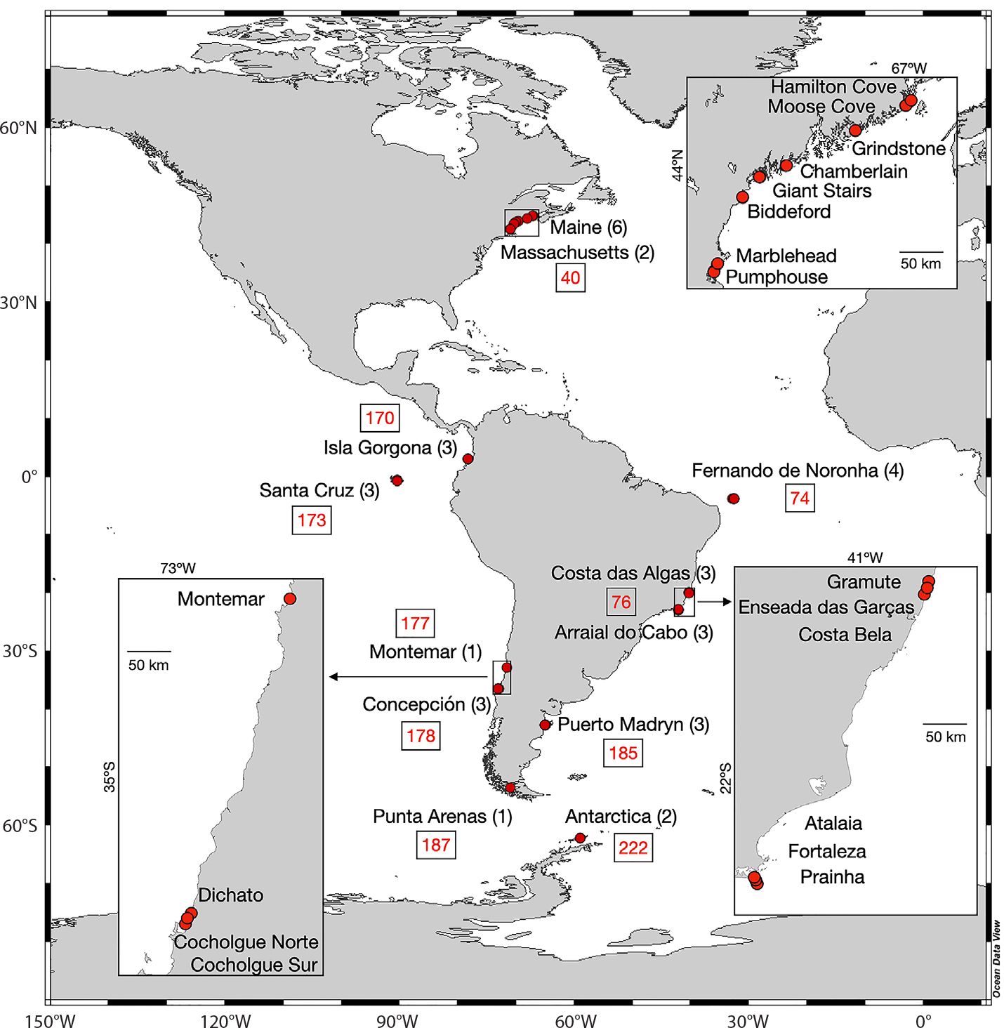
Figure 1. Marine Biodiversity Observation Network Pole to Pole of the Americas (MBON Pole to Pole) localities contributing data to this study. Surveys were carried out in the United States, Colombia, Ecuador (Galápagos Islands), Brazil, Argentina, Chile, and Antarctica (see Table 1) encompassing ten Marine Ecoregions of the World (MEOW) highlighted with red numbers: Gulf of Maine (40), Panama Bight (170), Eastern Galápagos Islands (173), Fernando de Noronha and Atol das Rocas (74), Eastern Brazil (76), Central Chile (177), Araucanian (178), Patagonian Shelf (185), Channels and Fjords of Southern Chile (187), and South Shetland Islands (222). Numbers in parentheses indicate the number of sampling sites surveyed at each locality. Inset maps show areas highlighted with rectangles containing sampled localities separated by more than 10 km within a country. > High res figure

 

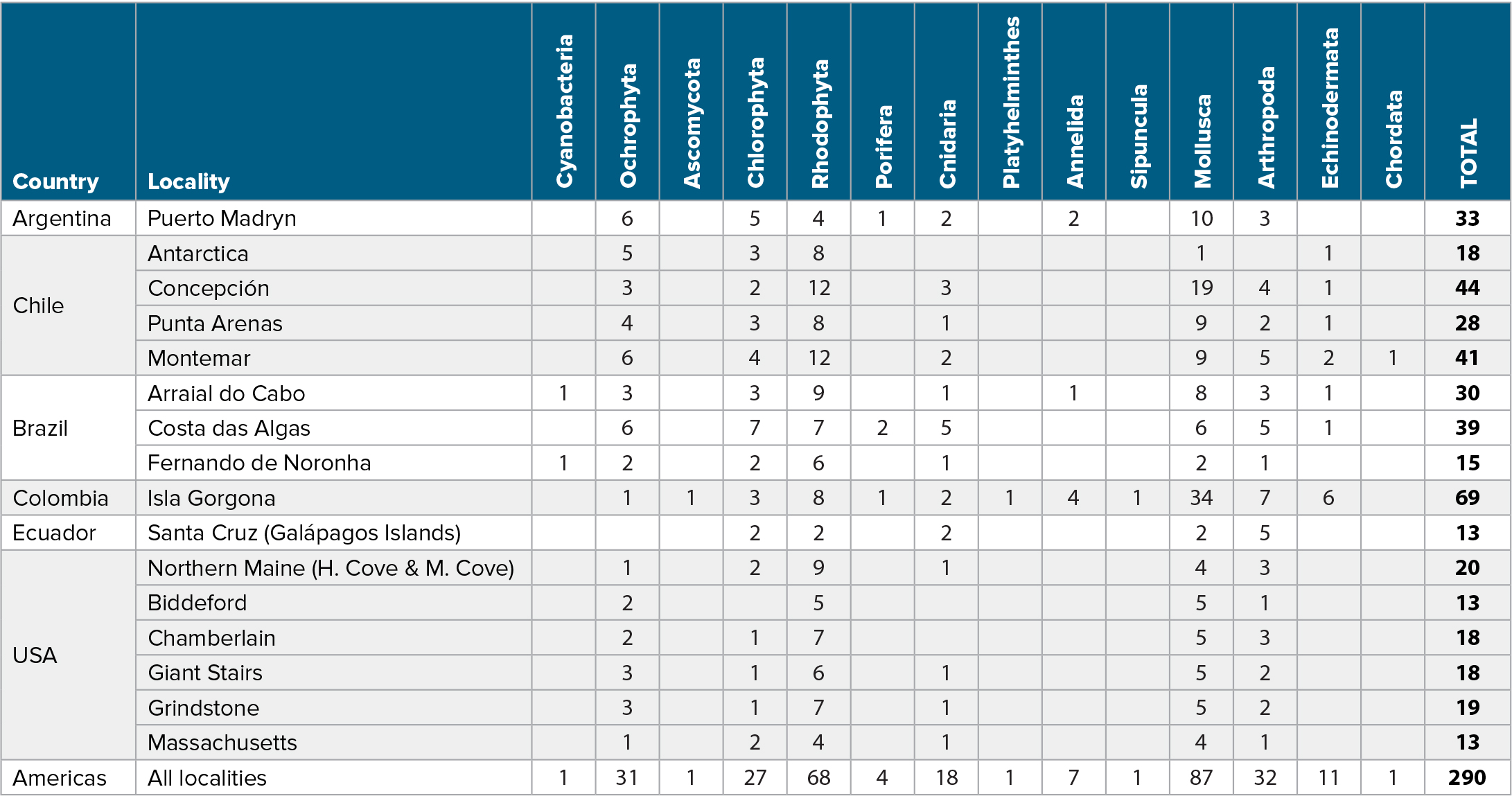
Table 1. Taxonomic records per phylum (or equivalent) collected across surveyed sites. > High res table

 

METHODS

Rocky Intertidal Biodiversity Surveys

Sessile and slow-moving macroinvertebrates and algal communities from 34 sites distributed across 16 localities that occupy 10 biogeographic ecoregions of the Marine Ecoregions of the World classification (MEOW; Spalding et al. 2007) were surveyed from July 13, 2018, through March 29, 2019 (Figure 1, Table S1). Surveys were carried out following a standardized protocol of the SARCE program (SARCE, 2012; Miloslavich et al., 2010, 2011; Cruz-Motta et al., 2020) and modified by the participants in the MBON Pole to Pole program. In each country, one or several localities separated by 30–100 km were surveyed. Within each locality, up to three sites separated by no more than 5 km were sampled. Sites were chosen to be representative of locations/regions based on previous knowledge of investigators and available literature regarding local patterns of rocky shore diversity, aiming to be representative of local intertidal fauna and flora. Recommendations on similarities in oceanographic and geomorphological features among sites within localities were also assessed previous to site selection. In general, all sites are semi-exposed shores with similar aspects within locations. Criteria of ease of access, level of protection (e.g., marine protected areas), and previous sampled sites were also considered in selection but not mandatory or decisive for site choice. All those recommendations are described in the revised version of the SARCE protocol cited above (i.e., Cruz-Motta et al., 2020).

At each site, ten 0.5 × 0.5 m quadrats were randomly distributed across tidal strata (high, mid, and low) for a total of 30 quadrat observations collected per site, with few exceptions (see Table S1). On average, quadrats were placed between ~1 and several tens of meters apart, depending on the geomorphological characteristics of surveyed sites and accessibility of sampled areas. Each site was divided into three strata (tidal levels) parallel to the coastline using the almost universal biologically based characteristics of rocky shores of high, mid, and low zones. For example, in central Chile (Montemar; Figure 1), the presence of Mazzaella laminarioides is used as an indicator species of the mid-tide level, barnacle species such as Balanus leavis or Jhelius cirratus are representative for high tide, and Fissurella crassa for low tide. In Brazil, the classification for intertidal zones was based on Coutinho (1995), where the zone dominated by the barnacle Chthamalus bisinuatus marks the upper limit of the mid-​littoral, the barnacle Tetraclita stalactifera indicates the middle part of the mid-littoral, and the upper limit of the macro-algae Sargassum spp. indicates the lower boundary of the intertidal zone. In Isla Gorgona (Colombia), species like Nerita scabricosta and various litorinids demark the ranges of the high intertidal, whereas the mid intertidal is characterized by the presence of Vassula melones and Nerita funiculata, and the low intertidal by the presence of several small green and red algae and the snail Turbo saxosus. The US sites were surveyed at high- and mid-tide habitats only due to logistical challenges of sampling in the low intertidal zone at sites with very large (up to 6–7 m) tidal amplitudes.

Number of organisms and percent cover of major taxonomic entities were reported for each quadrat by using the point intercept method in a 10 × 10 grid with 100 intersect points evenly spaced. Percent cover estimates included sessile organisms such as barnacles, mussels, some colonial invertebrates (including zoanthids and ascidians), and algal turfs or macroalgae. Only organisms below intersect points were registered with this protocol. Rare species were recorded if they were present below the intersection point within each quadrat. This method is primarily intended for assessing rapid changes in the relative abundance of dominant species and is limited in its power for detecting minute compositional changes. Organisms were visually identified in the field to the lowest possible taxonomic level (see Figure S1). For this study, we only used presence/absence information. Data from the surveys were uploaded and made available for public use on OBIS (see http://ipt.iobis.org/mbon/rss.do).

 

Coverage-Based Stopping of Biodiversity Data

To identify the minimum number of samples (e.g., quadrats) needed to characterize the biodiversity of a site, we implemented the coverage-based stopping rule from Chao and Jost (2012). This rule is based on the notion of sample coverage, or the completeness of the sampling. With data from a community composed of individuals, each belonging to a certain species, it is possible to compute the probability that collecting an additional sample would yield a new species. This value is based on the number of singletons and doubletons (i.e., samples with one or two species, respectively; Chao and Jost, 2012). A high proportion value implies that additional samples might yield new “information,” because the system appears to have many rare species. In this case, the survey would be considered to have “low coverage” because it is not complete with respect to the total biodiversity implied by the data.

The species-sampling or rarefaction curve (Simberloff, 1978; Magurran, 2003; Chiarucci et al., 2008) of such sites would show a steep slope as counts start, uncovering many new species (i.e., the expected increase in diversity per quadrat taken). Eventually, however, the community will have been exhaustively censused, and further sampling will yield fewer new species: this is the point along the curve where the slope will approach zero (i.e., the saturation point). A sample with low coverage would fall along the steep part of the curve, where the slope is largest and the probability of uncovering new information is highest. A sample with high coverage would fall along the end of the curve, where the slope is smallest. A sample with total coverage (100%) would occur at the saturation point.

Chao and Jost (2012) proposed interpolating (rarefying) and extrapolating biodiversity estimates to quantify the entirety of the curve, including a bootstrapping procedure to determine confidence intervals. They argued that coverage can be computed for any degree of sampling effort, regardless of whether effort was to be expanded. A stopping point for sampling would be identified as the number of samples where coverage reaches a certain level. This point will vary depending on the rarefaction curve: if the curve rises rapidly, high or total coverage may occur with few samples, whereas if the curve is more gradual, many more samples (quadrats) would need to be collected to acquire the same degree of coverage.

We constructed interpolation-extrapolation curves using the iNEXT package in R using data from all 10 quadrats in each strata and site per locality (i.e., unnested) as the sample unit (Hsieh et al., 2016). Rarefaction curves computed with iNEXT are based on samples (quadrats), not individuals, and correspond to Chao2 estimates (and respective sample coverage). We set a stopping point at 90% coverage (i.e., 90% probability that repeated sampling would not yield any new species) and applied this threshold to a subset of our data. We implemented an open-source function (covstop) in R to identify the stopping point as number of quadrats (i.e., samples) for any user-​specified level of coverage.

 

Variation in Species Composition

In addition to total richness, the variability in taxa composition within and among communities can also be estimated. To optimize the sampling effort necessary for characterizing species composition of communities with a certain degree of precision, we calculated the multivariate standard error (MultSE; Anderson and Santana-Garcon 2015). This metric represents the precision with which the position of the centroid in a multivariate community space (using an appropriate dissimilarity index) is guaranteed for a specific sampling effort.

The process draws a random number of samples from a community and computes the MultSE. This procedure is repeated for an increasing number of samples. For few samples, each draw is likely to capture different species such that repeated draws would result in a highly variable positioning of the centroid in the multivariate space (i.e., low precision). As sample size increases, new samples reinforce the relative composition of species that are already represented by other samples in the multivariate space, and the MultSE converges toward zero (i.e., maximum precision). Reaching this value will imply a very high sampling effort. Hence, a compromise between minimum precision required and sampling cost must be defined a priori. The goal is to restrict the minimum sample size to that where MultSE is acceptable and affordable. By using this approach, we assume that different communities sampled with acceptable precision are inter-comparable regardless of the sampling effort applied to each.

Local variability in species composition strongly affects MultSE. This means that regions with high β diversity require more sampling effort than regions with low β diversity (Anderson and Santana-Garcon, 2015). Because the objective here is to compare changes in species composition along the rocky shores of the Americas, we propose that community composition estimates should be made using a common bounded measure of dissimilarity (i.e., Jaccard) and a common level of precision (i.e., 0.1). This provides two advantages: (1) the data are treated as presence/absence because only changes in species composition are of interest and trends in magnitude of abundances of dominant species will not affect the analysis, and (2) this index is constrained between 0 and 1 and thus interpretable in terms of proportion of shared species. With these, estimates of MultSE among very different sites can be compared, and optimal sampling efforts could be specified for each site with a survey-wide acceptable MultSE defined a priori (e.g., 0.1, which is roughly analogous to a 90% level of coverage). Simulation and resampling procedures were conducted using the SSP R package (Guerra-Castro et al., 2021).

 

RESULTS

The number of taxonomic records collected in each of the 34 MBON Pole to Pole survey sites varied between a minimum of 24 at Ratonera (Santa Cruz, Galápagos Islands in Ecuador) to a maximum of 215 in Arraial do Cabo in Brazil and Puerto Madryn in Argentina (Figure 2 and Table S1). Sampling effort was generally comparable among localities, with an average of ~25 quadrats collected per survey over the three strata: high, mid, and low tide. The highest and lowest taxonomic richness readings were observed at Isla Gorgona (Colombia; 69 species), and in the Galápagos Islands (Ecuador; 13 species) (Table 1). The second lowest species richness was observed in the island of Fernando de Noronha (Brazil). On average, ~78% of taxonomic records collected in this study were identified to species level, ~19% to genus, and less than 3% to a higher taxonomic rank (Figure S1).

 

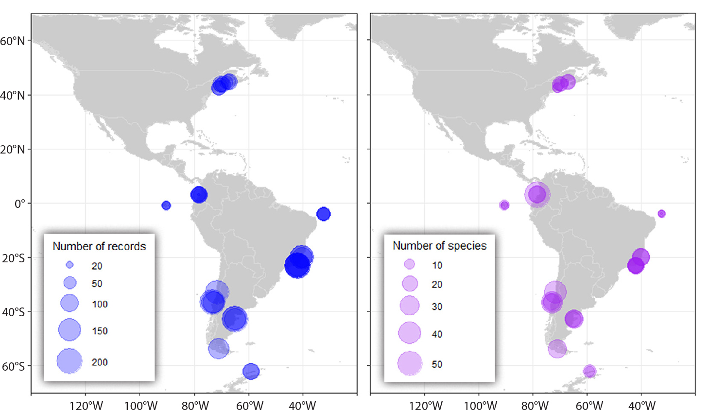
Figure 2. Number of taxonomic occurrences (records; left panel) collected at 16 localities across the region. Localities have more than one survey site, except for two localities in Chile and four localities in the United States. Right panel shows total number of species (richness) observed during these surveys at corresponding localities shown in Figure 1. > High res figure

 

Rarefaction curves derived from survey data indicate varying levels of species richness coverage at sampled localities (Figure 3). On average, species richness coverage at high- and mid-tide strata was ~90% relative to maximum extrapolation values (end of dotted line in Figure 3). This value dropped to ~84% in the low tide stratum. At most localities, surveys detected >80% of the species, except within specific strata in Santa Cruz, Biddeford, Isla Gorgona, and Montemar where coverage values were ≤76%, suggesting under­sampling with respect to the total amount of implied biodiversity. Results also suggest a large degree of oversampling in a number of localities as evidenced by the number of samples collected beyond asymptotic points of species saturation curves (Figure 3). For example, Antarctica and Fernando de Noronha appeared to be significantly oversampled at high- and mid-tide strata by at least twofold, where ~5 or fewer quadrats would allow detection of at least 90% of the species in these communities. These results are further supported by simulation experiments showing that species richness values in randomly selected samples over increasing sampling effort are in good agreement, and within similar ranges, with rarefaction curves computed with the iNEXT package (Figure S2).

 

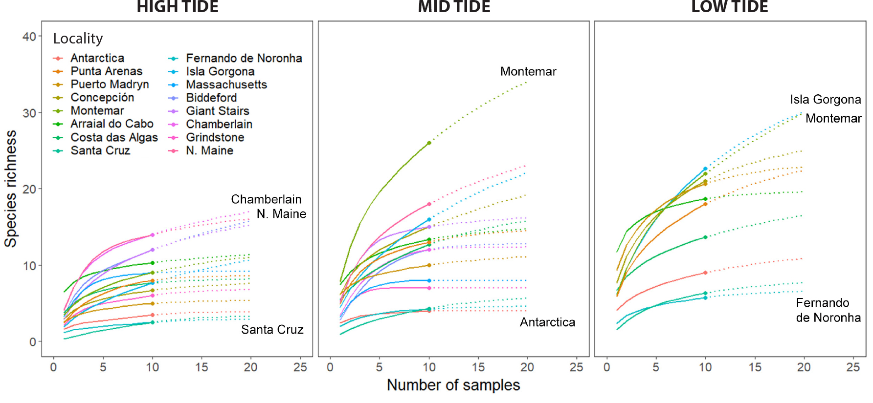
Figure 3. Rarefaction curves showing interpolated and extrapolated species richness (continuous and dotted lines, respectively) as a function of the number of samples (quadrats) taken at each locality, and further parsed by vertical strata (high, mid, and low intertidal). Dots on each curve represent the actual number of samples collected. > High res figure

 

By applying coverage-based stopping, the minimum number of samples required to estimate species richness at each locality was lower than the actual number of quadrats collected, indicating that there was significant oversampling across surveyed areas (Figure 4). Over-collection of samples varied between ~20% and several fold over the minimum required value, which was as high as ~fivefold at the high- and low-tide strata in Arraial do Cabo, Brazil. Twenty-five percent of localities were under­sampled by as much as ~50% (mid-tide stratum of Montemar and Isla Gorgona) with respect to the 90% coverage-based stopping value (Figure 4; see Table S2). Of these, Isla Gorgona (Colombia) was consistently undersampled at all strata, followed by Montemar in Chile, and the high- and mid-tide strata within several localities in Maine (USA) exhibited comparable undersampling levels.

 

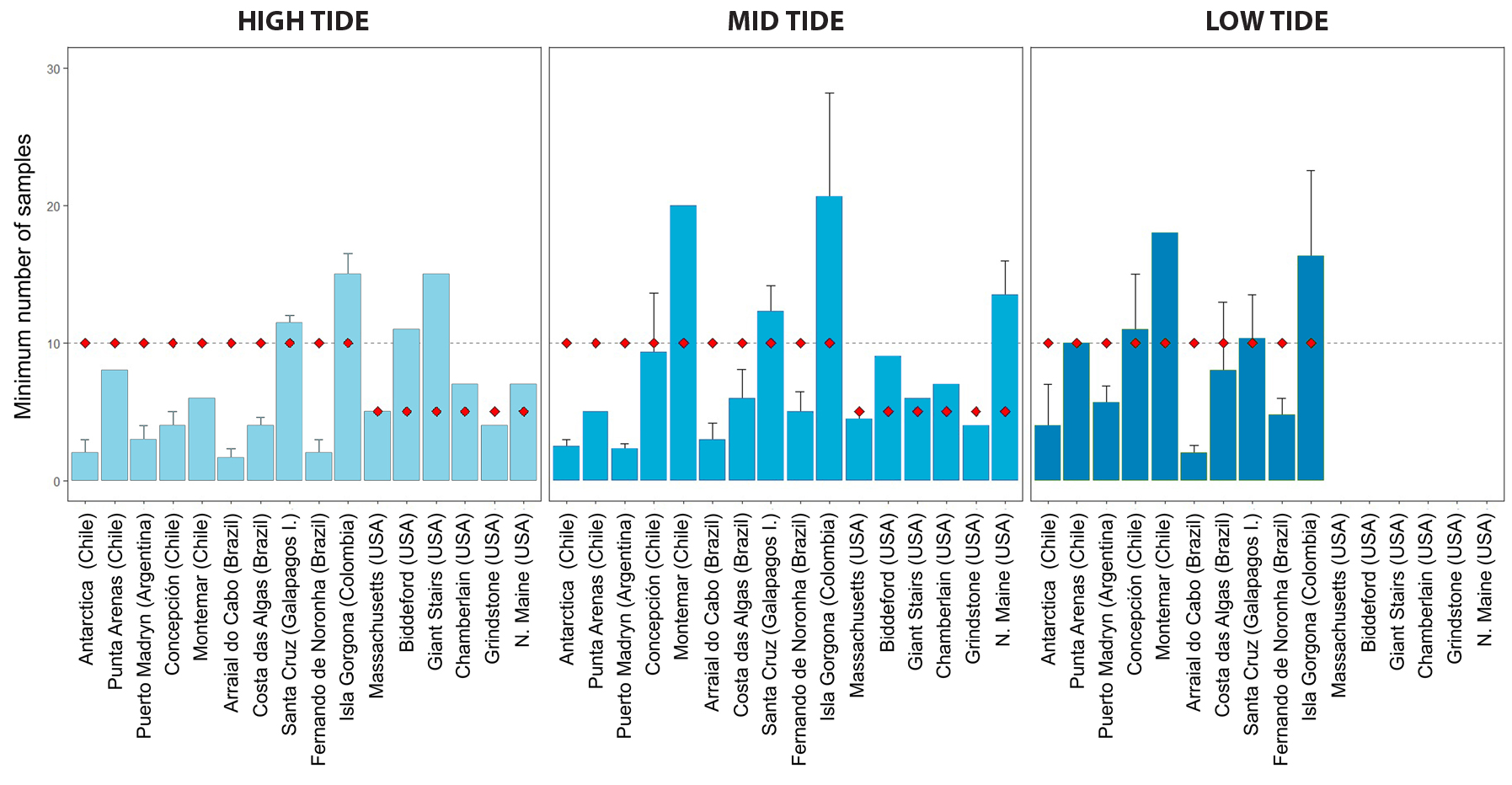
Figure 4. Bar plots showing predicted number of samples (based on coverage-​based stopping; see description in text) required at each locality to reach 90% coverage of species richness using the Covstop R function. The horizontal dashed line indicates the standard number of samples (n = 10) recommended by the sampling protocol, and the red diamonds indicate the actual number of samples collected at each locality. Bars are plotted from left to right according to latitude. > High res figure

 

Two localities showed MultSE <0.1 within the high-tide strata with two quadrats only (i.e., high tide in Grindstone, USA, and Fernando de Noronha, Brazil; Figure 5). Chamberlain (USA; high tide), Montemar (Chile; mid tide), and Isla Gorgona (Colombia; low tide) required the highest number of samples, with up to 16 quadrats, to achieve a MultSE uncertainty of 10%. The required sampling effort at low tide, where species richness is generally highest, was comparable at all localities. This is apparent by MultSE curves being closer in most low tide strata than in higher strata (Figure 5). Nonetheless, the majority of localities were oversampled, especially those for which the MultSE curves never intersected the 0.1 threshold.

 

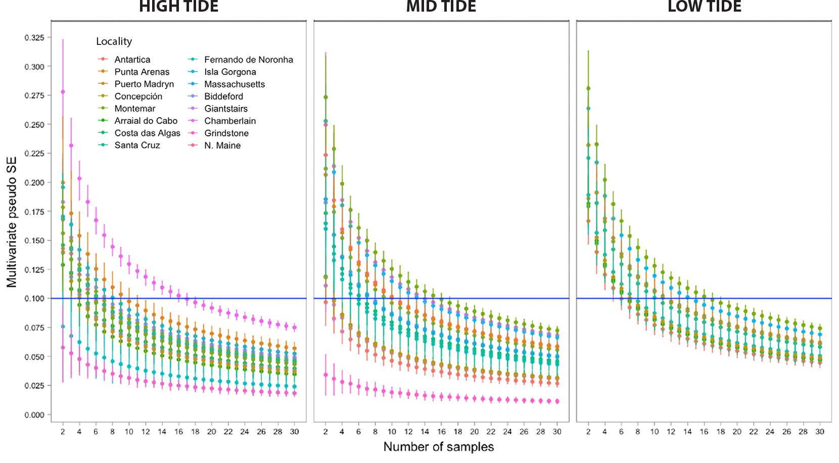
Figure 5. Number of samples required to characterize benthic community composition for sites in each locality with uncertainty levels below 0.1 multivariate pseudo standard error (MultSE) estimated using simulations and Jaccard dissimilarities. Symbols indicate MultSE versus sampling effort (number of samples) at the three strata per locality. Most localities have more than two sites sampled; for these cases, the MultSE was obtained using the residuals of a linear model as variance. Symbols are colored according to locality. Error bars show upper and lower limits of MultSE based on randomized resampling over simulated data at the corresponding sampling effort level. The horizontal blue line indicates the 0.1% MultSE threshold. > High res figure

 

DISCUSSION

We demonstrate that it is often easy to oversample during surveys of benthic biodiversity and community composition across rocky shores. However, at some sites, undersampling is also common. Therefore, a simple and quick method to assess sampling effort can help optimize resources. Such an approach will be “front loaded,” requiring adoption of these methods the first time a site is sampled. They can then provide guidance for repeated sampling at that same location over time.

The approach presented here is driven as much by practical limitations as by statistical or ecological ones. It is not possible to deploy equivalent effort everywhere (Adenle et al., 2015; Titley et al., 2017), even though many rocky shores are biodiversity “hotspots” that are in greatest need of standardized monitoring (Kim and Byrne, 2006; Giam et al., 2010). If we start from this perspective—that due to varying capacity and institutional support, effort must and, indeed, already does differ from locality to locality—then our proposed approach is not only advisable but unavoidable. The key advance consists in using validated statistical methods, such as fixed-coverage stopping and MultSE, to produce data-driven recommendations on replication and generate unbiased indicators of biodiversity. To that end, R packages used in this study will aid others in making defensible and cost-effective decisions in deploying or adjusting ongoing biodiversity monitoring.

We note that there is an additional opportunity to adopt an unbalanced sampling approach to reassign existing effort. For example, if participants at each site were previously asked to take n = 10 samples by strata, and our data suggest only a minimum of three to five samples is necessary, then each participant could conceivably reallocate the remaining samples to a different site or time, if they are still capable of collecting 10 samples. This solution, therefore, increases the potential spatial and temporal extent of the network while asking no more of partners than they were willing and able to contribute initially. It not only provides opportunity to expand the spatial and/or temporal footprint of the surveys but also may increase data collection along shores whose access is limited by extreme tides.

We advise some caution in implementing these two techniques, in that they are based on existing data. Drastic changes to the system—for example, through disturbance or invasive or range-expanding species—might dictate more or less sampling in subsequent years. We make two recommendations along these lines. First, we suggest building in a reasonable buffer to anticipate future changes by moderately increasing replication (say, by 10%–20%; see Table S2). Thus, if the suggested number of samples is n = 8, it would be advisable to take one to two extra samples as long as it is logistically feasible. Second, practitioners are advised to reevaluate their design after each survey period. By continually incorporating new data, the optimal suggested sample size will become more precise and less likely to under- or oversample changing communities at a particular locality. Finally, we acknowledge that in heavily skewed communities with many rare species and very low evenness, such methods are known to underperform (Brose et al., 2003), so we urge caution on the part of the investigators to consider the application of these techniques depending on the characteristics of their systems. The proposed approach should be carefully evaluated under extreme scenarios, for example, in highly uneven communities, where these methods (and indeed many others) could lead to inaccurate richness estimates and would likely fail to capture most (i.e., >60 %) of the actual diversity. Nonetheless, the likelihood of occurrence of extremely unbalanced communities is generally very low and, therefore, we are confident that these methods are appropriate for collaborative ecological survey networks such as MBON Pole to Pole.

 

Coverage-Based Stopping Versus MultSE Estimates

As expected, our analysis confirms that the level of sampling effort required to produce comparable measures of biodiversity for the rocky shores of the Americas varies between localities and tidal strata and depends on the diversity component used (species richness or α diversity, and species composition or β diversity). Nonetheless, while communities at most sites surveyed in this study are likely well characterized with the level of sampling effort recommended by the SARCE protocol (i.e., 30 quadrats per site), several of these sites appeared to be oversampled across different tidal strata whereas others were undersampled and thus remain not fully characterized for α and β diversity.

We identified a predictable relationship between sampling effort required for a desired sample coverage (e.g., 90%) and a desired MultSE below 0.1, with correlation coefficients (R) values varying between 0.75 and 0.93 (p << 0.01) in the mid- and low-tide strata, respectively (Figure 6). Correlation slopes above the 1:1 ratio indicate that characterizing α diversity with a 90% coverage would generally require more samples (quadrats) than for estimations of β diversity (species turnover) with a MultSE <0.1. Specifically, differences in sampling effort estimates between these approaches could be the result of three distinct scenarios. In the first one, local richness and multivariate dispersion increase moderately with each new quadrat sampled. This scenario reflects turnover of species in the entire community; such cases can be identified as points near to the dashed line in Figure 6. A second situation could show local richness increasing substantially with each new quadrat sampled while multivariate dispersion reaches an asymptote. In this scenario, moderate species turnover would occur with a significant proportion of singleton species. The effect of shared species over the multivariate dispersion is stabilization of MultSE with few samples regardless of the high frequency of singleton species. However, singleton species have a greater effect in the estimation of sample coverage and can therefore lead to a substantial difference in sampling effort estimates. This case corresponds to points far above the dashed line in Figure 6. In the third situation, local richness increases negligibly with each new quadrat, but multivariate dispersion keeps increasing. This scenario would translate into high local nestedness of species and corresponds to points far below the dashed line in Figure 6. Here, coverage-based stopping should yield comparatively lower number of quadrats needed. These results indicate that sampling effort may also vary depending on the diversity component of interest (e.g., α and β diversity). Hence, by applying the largest sampling effort estimate from either approach will allow to obtain the most accurate sampling effort at each locality (see Table S2).

 

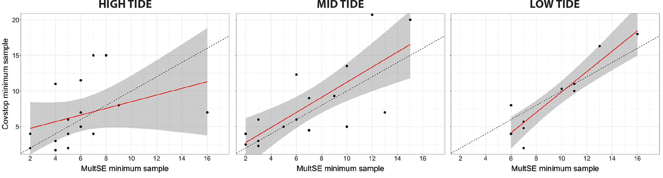
Figure 6. Minimum number of samples needed to characterize community composition with uncertainty levels below 10% multivariate pseudo standard error (MultSE) versus those required to achieve 90% coverage of species richness (coverage-based stopping), at high, mid, and low tide strata. The black dotted lines indicate the 1:1 baselines, the red lines show the linear regression between minimum samples from the two methods, and the shaded areas indicate the standard error of the regression. > High res figure

 

Latitudinal Diversity Patterns

We found that MBON Pole to Pole sites around the equator, specifically Santa Cruz (Galápagos Islands; 0.751°S, 90.315°W) and Fernando de Noronha (Brazil; 3.846°S, 32.418°W), showed the lowest richness values for rocky shore communities (Figure 7). Rocky intertidal zones in some tropical areas have been described as species poor and dominated by encrusting forms (Brosnan, 1992). Furthermore, Cruz-Motta et al. (2020) found that sessile macrofaunal communities of rocky intertidal zones along the Pacific and Atlantic coasts of South America show linear or unimodal latitudinal gradients in α diversity (species richness) of opposite direction to the expected inverse relationship with latitude; diversity appears to decrease from temperate to tropical latitudes. They also found a similar relationship between β diversity, a proxy for shifts in community composition, and latitude most likely driven by species turnover. A plausible explanation for the low diversity observed at these localities is that Fernando de Noronha and Santa Cruz are remote islands located at >300 km and >1,000 km from the continent, respectively, and therefore are subject to low immigration rates due to high degrees of geographic isolation (Quimbayo et al., 2019). Low species richness here could also result from high post-settlement mortality, which would inflate the role of local diversity and decrease the role of the regional species pool. Additionally, both island systems are of volcanic origin dating from Miocene and Pliocene epochs and thus are relatively young in terms of evolutionary timescales (Simkin, 1984; Mohriak, 2020). This is consistent with previous studies reporting low species richness in the Galápagos Islands relative to other tropical areas for fish and macroinvertebrates, likely resulting from geographic isolation and therefore low rates of species immigration (Stuart-Smith et al., 2013; Edgar et al., 2004; Barnes, 2017). Seasonal shifts in ocean productivity can also affect species richness and abundance in these islands. The Galápagos archipelago is characterized by marked seasonality with warm, nutrient-poor waters occupying the region during the austral summer and fall months, followed by cooler, nutrient-rich waters in the winter-spring season (Palacios, 2004). Therefore, low species richness observed in this study likely resulted from surveys being carried out during March 27–29, 2019, the peak of the warm season when productivity tends to be significantly lower than during subsequent colder and more productive months. Surveys reported by Gelin et al. (2003) observed considerably higher species richness in Santa Cruz, possibly due to higher recruitment levels and macro­algae percent cover, as surveys in their study were conducted during the onset of the productive season in the month of May (2001). Furthermore, surveys in Santa Cruz for this study were carried out in March 2019 and coinciding with El Niño (ONI +0.7) conditions. By contrast, we found that algal cover and overall biodiversity were notably greater in March 2021, when a weak La Niña (ONI –0.8) was present. Clearly, these rocky intertidal communities can exhibit major shifts in species richness and composition over seasonal cycles and interannually that should be accounted for when determining sampling effort with coverage-based stopping and MultSE estimates.

 

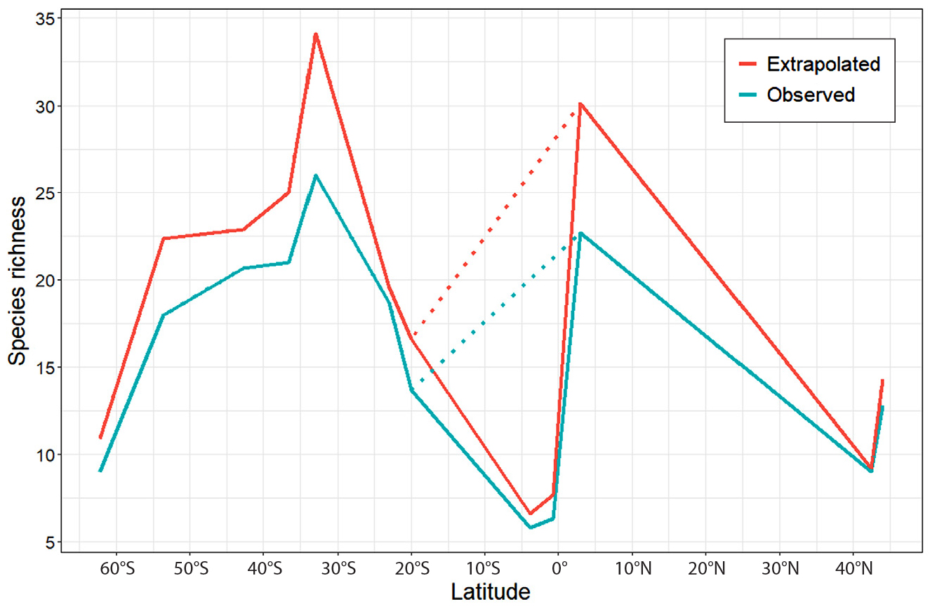
Figure 7. Species richness (observed and extrapolated) versus latitude. Extrapolated richness corresponds to maximum values across strata and averaged over sampled sites using the iNEXT package. Observed value corresponds to maximum richness values across strata and averaged over sampled sites (see Table S1). The dotted lines show distribution of species richness excluding site observations from remote island localities, Fernando de Noronha (Brazil) and Santa Cruz (Galápagos Islands). > High res figure

 

Species richness from surveys of this study was highest at ~33°S (Montemar, Chile). High species diversity in intertidal macro-invertebrate and algal communities of temperate zones has been attributed to the convergence of oceanic currents and the high productivity observed in these areas (Camus, 2008; Stuart-Smith et al., 2013; Gillman et al., 2015; Edgar et al., 2017; Cruz-Motta et al., 2020). Local properties such as isolation, environmental stress, and productivity appear to strongly influence diversity irrespective of the larger spatial gradient. Thus, adjusting sampling effort for each site or locality should be considered in monitoring designs.

 

Lessons Learned from a Collaborative Network

Demonstrating the utility of coverage-based stopping and MultSE analysis ultimately seeks to aid biodiversity monitoring programs in finetuning resources and augmenting their observational capacities to enhance sampling frequency and spatial coverage. Indeed, using the appropriate temporal scales is critical for avoiding aliasing and for effectively detecting biodiversity trends in rocky shore communities as well as associated drivers of change, as these habitats can be highly sensitive to seasonal environmental shifts and climate cycles (Rilov et al., 2021; Weitzman et al., 2021). As in other habitats, appropriate spatial scales and nested observations are crucial for accurately characterizing rocky intertidal communities over large geographic domains such as the Americas. While the field methodology adopted by MBON Pole to Pole aggregates observations over nested spatial units (from local to regional), the spatial resolution used is likely insufficient to accurately resolve horizontal variability of communities in regions with highly dynamic oceanographic regimes and strong seasonality, for example, the Galápagos Islands, Patagonia, or Antarctica. Furthermore, optimal extrapolation of species richness and species coverage estimates within a region requires that sampling localities be carefully selected based on well-defined environmental conditions in monitored areas, and that localities aggregate more than one site as small spatial representations of the characteristics of such region. When sharp environmental gradients are present, the hierarchical sampling design adopted by MBON Pole to Pole helps minimize spatial biases by pooling observations solely from distinct biomes. Tools for data-driven and objective sampling optimization presented in this study can enable the inclusion of additional “sites” and “localities” across the region to better resolve patterns of biodiversity within and across biomes along broad latitudinal gradients. Spatial biodiversity patterns reported in this study (and others; e.g., Cruz-Motta et al., 2020) should be periodically reexamined as more observations become available and with more complete knowledge of biodiversity distributions at surveyed sites and regions.

A key question is whether reducing the required number of samples needed to guarantee 90% of species coverage in oversampled localities translates into meaningful effort optimization for monitoring programs participating in collaborative networks like MBON Pole to Pole. We found that the time required for sampling often depends on the onset of the rising tide. For example, tidal rise is usually accompanied by strong wave action in localities with high-amplitude tidal ranges (i.e., Chile and the Gulf of Maine). Wave action can also be problematic in remote island localities like Fernando de Noronha where sea conditions challenge the completion of surveys within reasonable timeframes. In these areas, reducing the number of quadrats may help shorten survey times by several hours and ensure their completion. Moreover, collecting fewer samples can minimize the risk of surveys being delayed or interrupted for several consecutive days as a result of poor weather conditions. For example, in addition to high tidal range, heavy rain or exposure to high solar radiation at Isla Gorgona (Colombia) can affect sampling conditions for several hours or even days. This can be problematic as field expeditions must often be completed within a single day due to logistical or budgetary constraints. In areas with extreme weather conditions such as Antarctica, surveys are usually restricted to a very narrow time window, and thus collecting fewer samples at a site could enable increasing the spatial resolution by adding observations at new sites.

In most countries participating in MBON Pole to Pole, adding an extra day of fieldwork often translates into increasing costs to programs. Completing surveys quickly is a critical consideration for self- or partially funded efforts that would benefit from collecting additional observations and may enable the inclusion of surveys in habitats not constrained by tides (e.g., subtidal monitoring) in their study areas. Most of the investigators engaged in the MBON Pole to Pole network have been conducting surveys as supplementary or voluntary activities, and thus sampling optimization and site choice are critical considerations. The proposition of a reliable and adaptive methodology can help overcome these challenges, increase adherence and participation, and foster continuity of large-scale, collaborative monitoring efforts.

 

CONCLUSION

Applying equal sampling effort across monitoring sites is inefficient and, in some cases, may result in underestimation of the biodiversity of the areas. In the context of large-scale biodiversity networks, a unified balanced sampling design can be operationally unfeasible due to inequality of funding availability, personnel, and logistics, or ecological variance: heterogeneous regions, by their nature, require greater sampling effort than homogeneous regions. In this study, we provide two tools to compute optimal sample size based on species diversity and community composition. We highlight that future work should explore other measures of community variability and the use of simulations to extend inferences beyond observed data and assess uncertainty levels in the biodiversity of surveyed areas. As a consequence of our recommendation toward an unbalanced and adaptive survey design, we hope that more researchers, nations, and other entities are encouraged to become a part of such cooperative efforts. By potentially lowering the barrier to entry, networks may, paradoxically, generate more useful data overall than when asking participants to take a uniform number of samples. Ultimately, increased participation will lead to greater inventories of biodiversity through time and space, improving our understanding of this vital aspect of marine systems and providing the data necessary to properly conserve and manage it.

 

ACKNOWLEDGMENTS

This is a contribution to the Marine Biodiversity Observation Network (MBON) of the Group on Earth Observations Biodiversity Observation Network. The work was funded by NASA under the A.50 AmeriGEO Work Programme of the Group on Earth Observations with grant number 80NSSC18K0318 (Laying the foundations of the Pole-to-Pole Marine Biodiversity Observation Network of the Americas [MBON Pole to Pole]). The manuscript is also a contribution to the Integrated Marine Biosphere Research (IMBeR) project, which is supported by the Scientific Committee on Oceanic Research (SCOR) and Future Earth. Mention of trade names or commercial products does not constitute endorsement or recommendation for use by the US government. We would like to thank the Coordenação de Aperfeiçoamento de Pessoal de Nível Superior (CAPES), the Conselho Nacional de Desenvolvimento Científico e Tecnológico (CNPq), and the Long-term Program of Ecological Research (PELD) Coastal Habitats of Espírito Santo for the fellowship awarded to A.C.A. Mazzuco (88887.185758/2018–00; 88887.137932/2017–00; 031117341). Charles Darwin Foundation authors would like to thank the Gordon & Betty Moore Foundation for funding the staff time. This study was conducted under research permit GNPD No. PC-41-20. This publication is contribution number 2372 of the Charles Darwin Foundation for the Galápagos Islands. Financial support was received through Fondap-IDEAL grant 15150003 to E.C. Macaya. J.S. Lefcheck was supported by the Michael E. Tennenbaum Secretarial Scholar gift to the Smithsonian Institution. This is contribution no. 90 from the Smithsonian’s MarineGEO and Tennenbaum Marine Observatories Network. C.A.M.M. Cordeiro was supported by the fellowship granted by Fundação de Amparo a Pesquisa do Estado do Rio de Janeiro (FAPERJ - E-26/202.309/2019)

Montes, E., J.S. Lefcheck, E. Guerra-Castro, E. Klein, M.T. Kavanaugh, A.C.A. Mazzuco, G. Bigatti, C.A.M.M. Cordeiro, N. Simoes, E.C. Macaya, N. Moity, E. Londoño-Cruz, B. Helmuth, F. Choi, E.H. Soto, P. Miloslavich, and F.E. Muller-Karger. 2021. Optimizing large-scale biodiversity sampling effort: Toward an unbalanced survey design. Oceanography 34(2):80–91, https://doi.org/10.5670/oceanog.2021.216.

> Figures S1–S2 and Tables S1–S3 (977 KB pdf)

Adenle, A.A., C. Stevens, and P. Bridgewater. 2015. Global conservation and management of biodiversity in developing countries: An opportunity for a new approach. Environmental Science & Policy 45:104–108, https://doi.org/10.1016/​j.envsci.2014.10.002.

Allen, A.P., and J.F. Gillooly. 2006. Assessing latitudinal gradients in speciation rates and biodiversity at the global scale. Ecology Letters 9(8):947–954, https://doi.org/10.1111/j.1461-0248.2006.00946.x.

Alroy, J. 2010. Geographical, environmental and intrinsic biotic controls on Phanerozoic marine diversification. Palaeontology 53(6):1,211–1,235, https://doi.org/​10.1111/j.1475-4983.2010.01011.x.

Anderson, M.J., and J. Santana-Garcon. 2015. Measures of precision for dissimilarity-based multivariate analysis of ecological communities. Ecology Letters 18(1):66–73, https://doi.org/10.1111/ele.12385.

Barnes, D.K.A. 2017. Marine colonization and biodiversity at Ascension Island and remote islands. Journal of the Marine Biological Association of the United Kingdom 97(4):771–782, https://doi.org/​10.1017/S0025315415001526.

Barnosky, A.D., N. Matzke, S. Tomiya, G.O.U. Wogan, B. Swartz, T.B. Quental, C. Marshall, J.L. McGuire, E.L. Lindsey, K.C. Maguire, and others. 2011. Has the Earth’s sixth mass extinction already arrived? Nature 471:51–57, https://doi.org/10.1038/nature09678.

Beninger, P.G., I. Boldina, and S. Katsanevakis. 2012. Strengthening statistical usage in marine ecology. Journal of Experimental Marine Biology and Ecology 426–427:97–108, https://doi.org/10.1016/​j.jembe.2012.05.020.

Brose, U., N.D. Martinez, and R.J. Williams. 2003. Estimating species richness: Sensitivity to sample coverage and insensitivity to spatial patterns. Ecology 84:2,364–2,377, https://doi.org/​10.1890/​02-0558.

Brosnan, D.M. 1992. Ecology of tropical rocky shores: Plant-animal interactions in tropical and temperate latitudes. Pp. 101–131 in Plant-Animal Interactions in the Marine Benthos. D.M. John, S.J. Hawkins, and J.H. Price, eds, Oxford University Press, NY.

Brown, J.A., B.L. Robertson, and T. McDonald. 2015. Spatially balanced sampling: Application to environmental surveys. Pp. 6–9 in Procedia Environmental Sciences, vol. 27. A. Stein and D. Allards, eds, Special Issue on Spatial Statistics Conference 2015, https://doi.org/10.1016/​j.proenv.​2015.07.108.

Callaghan, C.T., A.G.B. Poore, R.E. Major, J.J.L. Rowley, and W.K. Cornwell. 2019. Optimizing future biodiversity sampling by citizen scientists. Proceedings, Biological Sciences 286(1912):20191487, https://doi.org/​10.1098/rspb.2019.1487.

Camus, P.A. 2008. Diversidad, distribución y abundancia de especies en ensambles intermareales rocosos. Revista de Biología Marina y Oceanografía 43(3):615–627, https://doi.org/​10.4067/S0718-19572008000300021.

Canonico, G., P.L. Buttigieg, E. Montes, F.E. Muller-Karger, C. Stepien, D. Wright, A. Benson, B. Helmuth, M. Costello, I. Sousa-Pinto, and others. 2019. Global observational needs and resources for marine biodiversity. Frontiers in Marine Science 6:367, https://doi.org/10.3389/fmars.2019.00367.

Caughlan, L., and K.L. Oakley. 2001. Cost considerations for long-term ecological monitoring. Ecological Indicators 1(2):123–134, https://doi.org/​10.1016/​S1470-160X(01)00015-2.

Chao, A., and L. Jost. 2012. Coverage-based rarefaction and extrapolation: Standardizing samples by completeness rather than size. Ecology 93(12):2,533–2,547, https://doi.org/​10.1890/11-1952.1.

Chase, J.M., B.J. McGill, P.L. Thompson, L.H. Antão, A.E. Bates, S.A. Blowes, M. Dornelas, A. Gonzalez, A.E. Magurran, S.R. Supp, and others. 2019. Species richness change across spatial scales. Oikos 128(8):1,079–1,091, https://doi.org/10.1111/oik.05968.

Chaudhary, C., H. Saeedi, and M.J. Costello. 2016. Bimodality of latitudinal gradients in marine species richness. Trends in Ecology & Evolution 31(9):670–676, https://doi.org/10.1016/​j.tree.2016.06.001.

Chiarucci, A., G. Bacaro, D. Rocchini, and L. Fattorini. 2008. Discovering and rediscovering the sample-​based rarefaction formula in the ecological literature. Community Ecology 9(1):121–123, https://doi.org/​10.1556/ComEc.9.2008.1.14.

Cornell, H.V., and S.P. Harrison. 2013. Regional effects as important determinants of local diversity in both marine and terrestrial systems. Oikos 122(2):288–297, https://doi.org/​10.1111/j.1600-0706.2012.20691.x.

Coutinho, R. 1995. Avaliação crítica das causas da zonação dos organismos bentônicos em costões rochosos. Oecologia Brasiliensis 1:259–271.

Cruz-Motta, J.J., P. Miloslavich, E. Guerra-Castro, A. Hernández-Agreda, C. Herrera, F. Barros, S.A. Navarrete, R.D. Sepúlveda, T.M. Glasby, G. Bigatti, and others. 2020. Latitudinal patterns of species diversity on South American rocky shores: Local processes lead to contrasting trends in regional and local species diversity. Journal of Biogeography 47(9):1,066–1,979, https://doi.org/​10.1111/jbi.13869.

Dornelas, M., N.J. Gotelli, B. McGill, H. Shimadzu, F. Moyes, C. Sievers, and A.E. Magurran. 2014. Assemblage time series reveal biodiversity change but not systematic loss. Science 344:296–299, https://doi.org/10.1126/science.1248484.

Duffy, J.E., L.A. Amaral-Zettler, D.G. Fautin, G. Paulay, T.A. Rynearson, H.M. Sosik, and J.J. Stachowicz. 2013. Envisioning a marine biodiversity observation network. BioScience 63(5):350–361, https://doi.org/​10.1525/bio.2013.63.5.8.

Edgar, G.J., S. Banks, J.M. Fariña, M. Calvopiña, and C. Martínez. 2004. Regional biogeography of shallow reef fish and macro-invertebrate communities in the Galápagos Archipelago. Journal of Biogeography 31(7):1,107–1,124, https://doi.org/​10.1111/j.1365-2699.2004.01055.x.

Edgar, G.J., T.J. Alexander, J.S. Lefcheck, A.E. Bates, S.J. Kininmonth, R.J. Thomson, J.E. Duffy, M.J. Costello, and R.D. Stuart-Smith. 2017. Abundance and local-scale processes contribute to multi-phyla gradients in global marine diversity. Science Advances 3(10):e1700419, https://doi.org/​10.1126/sciadv.1700419.

Giam, X., C.J.A. Bradshaw, H.T.W. Tan, and N.S. Sodhi. 2010. Future habitat loss and the conservation of plant biodiversity. Biological Conservation 143(7):1,594–1,602, https://doi.org/​10.1016/​j.biocon.2010.04.019.

Gillman, L.N., S.D. Wright, J. Cusens, P.D. McBride, Y. Malhi, and R.J. Whittaker. 2015. Latitude, productivity and species richness. Global Ecology and Biogeography 24(1):107–117, https://doi.org/10.1111/geb.12245.

Gelin, A., V. Gravez, and G.J. Edgar. 2003. Assessment of Jessica oil spill impacts on intertidal invertebrate communities. Marine Pollution Bulletin 46:1,377–1,384, https://doi.org/10.1016/S0025-326X(03)00368-0.

Guerra-Castro, E.J., J.C. Cajas, N. Simões, J.J. Cruz-Motta, and M. Mascaró. 2021. SSP: An R package to estimate sampling effort in studies of ecological communities. Ecography 44:561–573, https://doi.org/​​10.1111/ecog.05284.

Hessler, R., and H.L. Sanders. 1967. Faunal diversity in the deep-sea. Deep Sea Research and Oceanographic Abstracts 14(1):65–78, https://doi.org/​10.1016/0011-7471(67)90029-0.

Hoffmann, S., L. Steiner, A.H. Schweiger, A. Chiarucci, and C. Beierkuhnlein. 2019. Optimizing sampling effort and information content of biodiversity surveys: A case study of alpine grassland. Ecological Informatics 51:112–120, https://doi.org/10.1016/​j.ecoinf.2019.03.003.

Hsieh, T.C., K.H. Ma, and A. Chao. 2016. iNEXT: An R package for rarefaction and extrapolation of species diversity (Hill Numbers). Methods in Ecology and Evolution 7(12):1,451–1,456, https://doi.org/​10.1111/2041-210X.12613.

Kim, K.C., and L.B. Byrne. 2006. Biodiversity loss and the taxonomic bottleneck: Emerging biodiversity science. Ecological Research 21(6):794, https://doi.org/​10.1007/s11284-006-0035-7.

Lengyel, S., B. Kosztyi, D.S. Schmeller, P.-Y. Henry, M. Kotarac, Y.-P. Lin, and K. Henle. 2018. Evaluating and benchmarking biodiversity monitoring: Metadata-based indicators for sampling design, sampling effort and data analysis. Ecological Indicators 85:624–633, https://doi.org/10.1016/​j.ecolind.2017.11.012.

Lõhmus, A., P. Lõhmus, and K. Runnel. 2018. A simple survey protocol for assessing terrestrial biodiversity in a broad range of ecosystems. PLoS ONE 13(12):e0208535, https://doi.org/10.1371/​journal.pone.0208535.

Magurran, A.E. 2003. Measuring Biological Diversity, 1^st ed. Wiley-Blackwell, Malden, MA, 266 pp.

Miloslavich, P., J.M. Díaz, E. Klein, J.J. Alvarado, C. Díaz, J. Gobin, E. Escobar-Briones, J.J. Cruz-Motta, E. Weil, J. Cortés, and others. 2010. Marine biodiversity in the Caribbean: Regional estimates and distribution patterns. PLoS ONE 5(8):e11916, https://doi.org/10.1371/journal.pone.0011916.

Miloslavich, P., E. Klein, J.M. Díaz, C.E. Hernández, G. Bigatti, L. Campos, F. Artigas, J. Castillo, P.E. Penchaszadeh, P.E. Neill, and others. 2011. Marine biodiversity in the Atlantic and Pacific coasts of South America: Knowledge and gaps. PLoS ONE 6(1):e14631, https://doi.org/10.1371/​journal.pone.0014631.

Mittelbach, G.G., D.W. Schemske, H.V. Cornell, A.P. Allen, J.M. Brown, M.B. Bush, S.P. Harrison, A.H. Hurlbert, N. Knowlton, H.A. Lessios, and others. 2007. Evolution and the latitudinal diversity gradient: Speciation, extinction and biogeography. Ecology Letters 10(4):315–331, https://doi.org/​10.1111/j.1461-0248.2007.01020.x.

Mohriak, W. 2020. Genesis and evolution of the South Atlantic volcanic islands offshore Brazil. Geo-Marine Letters 40(1):1–33, https://doi.org/10.1007/s00367-019-00631-w.

Muller-Karger, F., M.T. Kavanaugh, E. Montes, W.M. Balch, M. Breitbart, F.P. Chavez, S.C. Doney, E.M. Johns, R.M. Letelier, M.W. Lomas, and others. 2014. A framework for a marine biodiversity observing network within changing continental shelf seascapes. Oceanography 27(2):18–23, https://doi.org/​10.5670/oceanog.2014.56.

Palacios, D.M. 2004. Seasonal patterns of sea-​​surface temperature and ocean color around the Galápagos: Regional and local influences. Deep Sea Research Part II 51(1–3):43–57, part of a special issue on Views of Ocean Processes from the Sea-viewing Wide Field-of-view Sensor (SeaWiFS) Mission: Volume 1, https://doi.org/10.1016/j.dsr2.​2003.08.001.

Pearlman, J., M. Bushnell, L. Coppola, J. Karstensen, P.L. Buttigieg, F. Pearlman, P. Simpson, M. Barbier, F.E. Muller-Karger, C. Munoz-Mas, and others. 2019. Evolving and sustaining ocean best practices and standards for the next decade. Frontiers in Marine Science 6:277, https://doi.org/10.3389/fmars.2019.00277.

Quimbayo, J.P., M.S. Dias, M. Kulbicki, T.C. Mendes, R.W. Lamb, A.F. Johnson, O. Aburto-Oropeza, J.J. Alvarado, A.A. Bocos, C.E.L. Ferreira, and others. 2019. Determinants of reef fish assemblages in tropical oceanic islands. Ecography 42(1):77–87, https://doi.org/10.1111/ecog.03506.

Rilov, G., N. David, T. Guy-Haim, D. Golomb, R. Arav, and S. Filin. 2021. Sea level rise can severely reduce biodiversity and community net production on rocky shores. Science of the Total Environment 791:148377, https://doi.org/10.1016/​j.scitotenv.2021.148377.

Rosenzweig, M.L. 1995. Species Diversity in Space and Time. Cambridge Core, Cambridge University Press, 460 pp., https://doi.org/10.1017/CBO9780511623387.

SARCE (South American Research Group on Coastal Ecosystems). 2012. Protocol and Sampling Design for Marine Diversity for the South American Research Group on Coastal Ecosystems. South American Research Group on Coastal Ecosystems, Caracas Venezuela, 12 pp., https://doi.org/​10.25607/​OBP-5.

Shimadzu, H. 2018. On species richness and rarefaction: Size- and coverage-based techniques quantify different characteristics of richness change in biodiversity. Journal of Mathematical Biology 77(5):1,363–1,381, https://doi.org/10.1007/s00285-018-1255-5.

Simberloff, D. 1978. Use of rarefaction and related methods in ecology. Pp. 150–165 in Biological Data in Water Pollution Assessment: Quantitative and Statistical Analyses. K. Dickson, J. Cairns, and R. Livingston, eds, ASTM International, West Conshohocken, PA, https://doi.org/10.1520/STP35663S.

Simkin, T. 1984. Geology of Galápagos. Biological Journal of the Linnean Society 21(1–2):61–75, https://doi.org/10.1111/j.1095-8312.1984.tb02053.x.

Spalding, M.D., H.E. Fox, G.R. Allen, N. Davidson, Z.A. Ferdaña, M. Finlayson, B.S. Halpern, M.A. Jorge, A. Lombana, S.A. Lourie, and others. 2007. Marine ecoregions of the world: A bioregionalization of coastal and shelf areas. BioScience 57(7):573–583, https://doi.org/10.1641/B570707.

Stuart-Smith, R.D., A.E. Bates, J.S. Lefcheck, J.E. Duffy, S.C. Baker, R.J. Thomson, J.F. Stuart-Smith, N.A. Hill, S.J. Kininmonth, L. Airoldi, and others. 2013. Integrating abundance and functional traits reveals new global hotspots of fish diversity. Nature 501(7468):539–542, https://doi.org/10.1038/nature12529.

Titley, M.A., J.L. Snaddon, and E.C. Turner. 2017. Scientific research on animal biodiversity is systematically biased towards vertebrates and temperate regions. PLoS ONE 12(12):e0189577, https://doi.org/​10.1371/journal.pone.0189577.

Turner, W.R., and E. Tjørve. 2005. Scale-dependence in species-area relationships. Ecography 28(6):721–730, https://doi.org/​10.1111/j.2005.0906-7590.04273.x.

Underwood, A.J. 1996. Experiments in Ecology: Their Logical Design and Interpretation Using Analysis of Variance. Cambridge University Press, Cambridge, 524 pp., https://doi.org/10.1017/CBO9780511806407.

Weitzman, B., B. Konar, K. Iken, H. Coletti, D. Monson, R. Suryan, T. Dean, D. Hondolero, and M. Lindeberg. 2021. Changes in rocky intertidal community structure during a marine heatwave in the northern Gulf of Alaska. Frontiers in Marine Science 8:115, https://doi.org/10.3389/fmars.2021.556820.

This is an open access article made available under the terms of the Creative Commons Attribution 4.0 International License (https://creativecommons.org/licenses/by/4.0/), which permits use, sharing, adaptation, distribution, and reproduction in any medium or format as long as users cite the materials appropriately, provide a link to the Creative Commons license, and indicate the changes that were made to the original content. Images, animations, videos, or other third-party material used in articles are included in the Creative Commons license unless indicated otherwise in a credit line to the material. If the material is not included in the article’s Creative Commons license, users will need to obtain permission directly from the license holder to reproduce the material.