Introduction
Earth is often defined by its extremes: the tallest mountain, the driest desert, the deepest ocean. In March 1875, during the first major expedition devoted primarily to the fledgling science of oceanography, the three-masted sailing corvette HMS Challenger of the Royal Navy discovered a deep depression in the seabed in the western Pacific Ocean—while en route to Guam, the ship had been blown off course to the west and serendipitously tracked over the southern end of the Mariana Trench. Traditional depth soundings were taken by the crew at regular intervals, the deepest of which indicated a depth of 8,140 m. Some 76 years later, during a three-year circumnavigation of Earth, HMS Challenger II, following its namesake, returned to the Mariana Trench, where its echo sounder recorded a depth of 10,863 m. To commemorate the discovery of the deepest trench in the world ocean by the two British ships, the deep depression in the southwestern Mariana Trench was named Challenger Deep.
While it is generally accepted that the deepest abyss in the ocean is indeed the Challenger Deep, the exact location and the depth of the very deepest spot are still topics of interest to the oceanographic research community. Much time, money, and intellectual energy have been invested in the development of techniques for measuring the deepest depth in the ocean (Gardner et al., 2014; Stewart and Jamieson, 2019), including the development of crewed submersibles capable of making the round trip to the bottom of the Challenger Deep. The first such descent was made on January 23, 1960, by the oceanographer Jacques Piccard and US Navy Lt. Don Walsh in the bathyscaphe Trieste (Piccard and Dietz, 1967; Walsh, 2009), whose onboard instruments indicated a depth of 11,521 m, although it was subsequently revised downward to 10,916 m. Over five decades later, on March 26, 2012, filmmaker and explorer James Cameron made the second crewed dive to the bottom of the Challenger Deep, a solo descent in his submersible DeepSea Challenger, and recorded a depth of 10,908 m (http://www.deepseachallenge.com/the-expedition/). More recently, on April 28, 2019, Victor Vescovo piloted his DSV Limiting Factor to a world record depth of 10,925 ± 4 m, and then made a second trip on May 1, 2019, becoming the first person to have descended to the bottom of the Challenger Deep twice (Cassie Bongiovanni, Caladan Oceanic, pers. comm., September 24, 2020; Stokstad, 2018; Fitzherbert, 2019; Taub, 2019;).
Since the 1951 Challenger II expedition, a wide range of estimates of the depth of the Challenger Deep have been reported in the peer-reviewed literature, mainstream periodicals, and cruise reports. In Figure 1, the published results are summarized while unpublished results are neglected for the sake of clarity. The published results are representative of the unpublished results, most of which come from cruise reports. The methods used to measure such extreme ocean depths, besides traditional sounding with a weighted rope or cable, have included explosives and stopwatches (Carruthers and Lawford, 1952; Gaskell et al., 1953), single-beam sonar (Hanson et al., 1959; Mantyla and Reid, 1978; Taira et al., 2004, 2005; Nakanishi and Hashimoto, 2011), multibeam sonar (Hydrographic Department and Japan Marine Safety Agency, 1984; Fujioka et al., 2002; Nakanishi and Hashimoto, 2011; Gardner et al., 2014; van Haren et al., 2017), side-scan sonar (Fryer et al., 2003), and pressure sensors (Piccard and Dietz, 1967; Todo et al., 2005; Bowen et al., 2009; 2012 James Cameron dive; Dziak et al., 2017; Fitzherbert, 2019). Gardner et al. (2014) and Stewart and Jamieson (2019) both provide a review of previous investigations of the deepest part of the ocean.
The seafloor in the Challenger Deep has been further divided into three distinct depressions, clearly evident from the clustering of measurements in Figure 1: the western, central, and eastern basins, each of which contend for the location of the greatest depth (see Figure 6 in Stewart and Jamieson, 2019, and Figure 3 in Gardner et al., 2014). Only one estimate of the corrected depth in the Challenger Deep exceeds 11,000 m. During the Soviet expeditions in 1957 and 1958 aboard R/V Vityaz, the vessel made several transects across the trench while operating a 10 kHz echo sounder (Hanson et al., 1959). Water-sampling bottles and thermometers were deployed to a depth of 10,200 m, acquiring temperature and salinity data from which a mean vertical sound speed profile was computed with the aid of an empirical equation (Hanson et al., 1959). The resultant estimate of the deepest depth was 11,034 ± 50 m. Taira et al. (2005), however, found that, when using the integrated sound speed profile as opposed to a water column average, a lower value of 10,983 ± 50 m is obtained, closer to the results of the numerous other investigators.
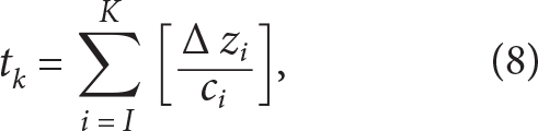
Figure 1. (a) Depth estimates in the West Basin (red), Central Basin (black), and East Basin (blue) of the Challenger Deep, Mariana Trench, and their uncertainties (if reported) taken from the peer-reviewed and popular literature, accompanied by (b) the respective positions of each measurement. The solid gray region is bounded by the 10,000 m depth contour and the area in the dashed outline is shown in (c)—the close-up of the Deep Sound Mk. II deployment and recovery positions, and the Deep Sound Mk. III deployment and approximate implosion positions. References: A = Carruthers and Lawford, 1952; Gaskell et al., 1953; Fisher, 1954. B = Hanson et al., 1959. C = Fisher and Hess, 1963. D = Piccard and Dietz, 1967; Nakanishi and Hashimoto, 2011. E = Fisher and Hess, 1963 (not shown); Fisher, 2009. F = Mantyla and Reid, 1978. G = Hydrographic Department and Japan Marine Safety Agency, 1984. H and I = Taira et al., 2005. J = Todo et al., 2005. K = Fryer et al., 2003. L = Fujioka et al., 2002. M = Nakanishi and Hashimoto, 2011. N = Bowen et al., 2009. O = Gardner et al., 2014. P = 2012 James Cameron dive. R = Dziak et al., 2017. S = van Haren et al., 2017. T and U = Cassie Bongiovanni, Caladan Oceanic, pers. comm., Sept. 24, 2020. (Note that the estimate in K was made using a combination of data from R/V Moana Wave in 1997 and R/V Melville in 2001. The position of E [R/V Spencer Baird, not shown] was made by a celestial fix, which can have errors of up to 2.2 km [Karl, 2007]; however, it was stated in Fisher and Hess [1963] that the measurement was in the western basin.) > High res figure
|
Time-of-flight measurements of impulsive acoustic signals from explosive shots and echo sounders require very well-constrained measurements of the speed of sound throughout the water column. In the past, before reliable deep-water-rated instruments were readily available, the sound speed profile over the full depth of the Challenger Deep was obtained from Matthew’s tables of sound speed (Matthews, 1939; Carruthers and Lawford, 1952; Mantyla and Reid, 1978; Zheng, 2015), comprising a compilation of historical measurements of water column chemistry by latitude and longitude. In modern times, direct measurements of the sound speed profile over the Challenger Deep have been made with conductivity, temperature, depth (CTD) sensors mounted on either deep submersibles or free-falling vehicles (Piccard and Dietz, 1967; Bowen et al., 2009; Taira et al., 2004; Barclay et al., 2017; Dziak et al., 2017; van Haren et al., 2017) and with expendable bathythermographs (XBTs; Fujioka et al., 2002; Gardner et al., 2014). Ideally, for depth estimation, such determinations of the sound speed profile should be concurrent with the acquisition of the time-of-flight data; otherwise, significant errors can arise in the acoustic estimate of the ocean depth (Beaudoin et al., 2009).
Here, we discuss how an imploding instrument enabled one of the deepest and most constrained estimates of the depth of the Challenger Deep. First, we discuss the expedition and the instruments used. We then outline the instrument deployment and implosion, followed by a discussion of the paths traveled by the shock wave generated by the implosion and the acoustic signal processing used to determine the time of arrival of multiple reflections of the shock wave. We then determine the depth of the Challenger Deep and the uncertainty in that depth estimate. Finally, we discuss how this estimate fits with other estimates of the Challenger Deep and the sources of uncertainty that can partially explain the discrepancies between different depth estimates.
The Expedition
In December 2014, a multidisciplinary expedition to the Mariana Trench on board Schmidt Ocean Institute’s R/V Falkor was led by Douglas Bartlett of Scripps Institution of Oceanography. Several autonomous, deep-diving instrument platforms were deployed in the central and eastern basins of the Challenger Deep with varying scientific objectives, including water sampling and CTD profiling throughout the water column, collection and video recording of hadal amphipods, and recording the broadband (5 Hz to 30 kHz) ambient sound over the full ocean depth on vertically and horizontally aligned pairs of hydrophones. Some of the findings from the expedition have been previously reported in the popular (Nestor, 2014) and scientific (Barclay et al., 2017; Lan et al., 2017) literature.
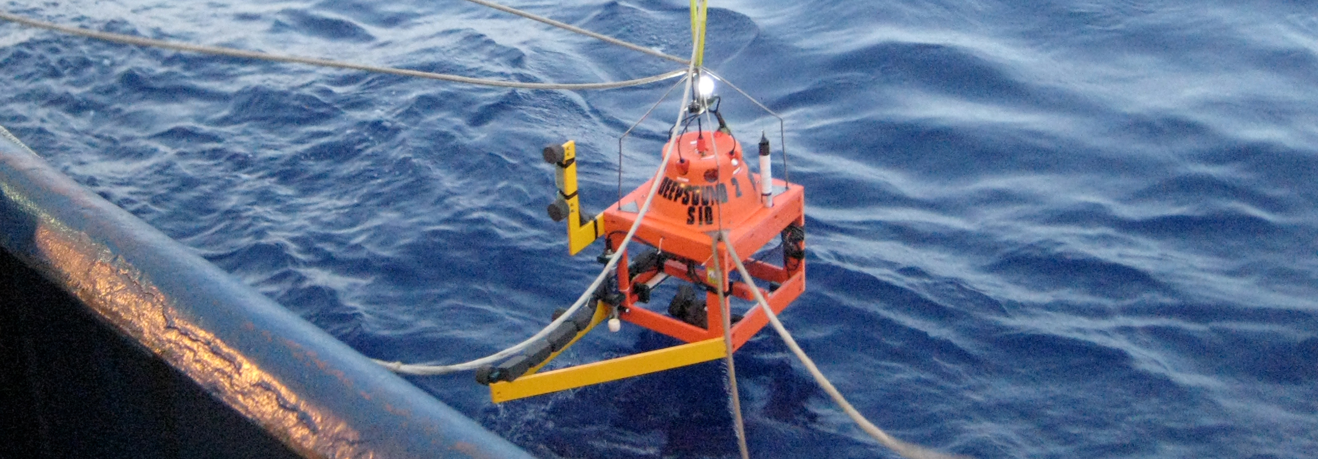
On December 17, 2014, we deployed two free-falling instrument platforms, designated Deep Sound Mk. II and Deep Sound Mk. III, into the Challenger Deep within about 25 minutes of one another. Each had a CTD profiler and multiple hydrophones on board, with system electronics contained in a 38 cm Vitrovex glass sphere pressure housing (Barclay and Buckingham, 2009). At a nominal depth of 9,000 m, during its descent to the bottom, the spherical pressure housing on Deep Sound Mk. III imploded, creating a highly energetic shock wave that reflected multiple times from the sea surface and the seafloor. The direct-path shock wave and several of the multi-path reflections were detected by the surviving instrument, Deep Sound Mk. II. The shock wave itself saturated the receivers on Deep Sound Mk. II and, consequentially, was unusable as a timing reference, but the arrivals of the multiply reflected impulses, which were much less energetic, provided accurate time-of-flight data for the full water column. When combined with the sound speed profile, obtained concurrently from the CTD on Deep Sound Mk. II, the multiple reflections provided the information necessary for estimating the depth of the Challenger Deep at the measurement site.
Deep Sound Mk. II and Mk. III
The Deep Sound instrument platforms (Figure 2) are deep-diving, autonomous profilers designed to descend under gravity until a pre-programmed condition is met, for instance, a pre-set depth, an elapsed time, or a minimum battery charge, at which point an iron drop weight is released, allowing the system to ascend to the surface under buoyancy, with a speed of 0.56 m s–1 in both directions. At the time of the R/V Falkor cruise in December 2014, the first of the Deep Sound systems, Mk. I, had been retired from service, but the remaining two, Mk. II and Mk. III, were both operational. The Vitrovex glass sphere installed on Mk. II was pressure rated to 9,000 m and that on Mk. III was specified to 11,000 m. Both systems had previously made successful descents to a depth of about 9,000 m (Barclay and Buckingham, 2014). In all three Deep Sound platforms, the control and data acquisition electronics, a bank of lithium-ion batteries, and the power management system are contained within the Vitrovex glass sphere, and a skeletal frame of titanium and high-density polyethylene (HDPE) provides an external structure on which various sensors, including hydrophones, could be mounted.
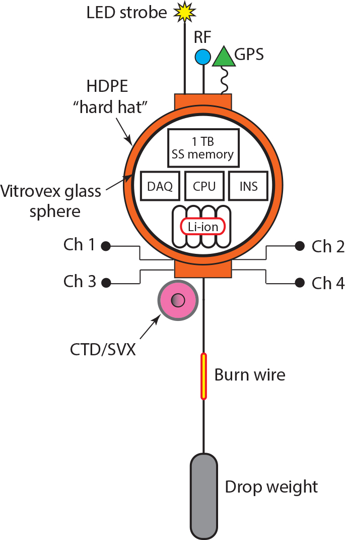
Figure 2. Schematic of Deep Sound Mk. III showing four hydrophone channels (not in operational configuration), three recovery antennas (LED, RF, GPS), and the CTD/SVX module. > High res figure
Ch X = Hydrophone channel number X
CPU = Central processing unit
CTD/SVX = CTD/sound velocity meter
GPS = Global Positioning System
HDPE = High-density polyethylene
DAQ = Data acquisition unit
INS = Inertial navigation system
LED = Light emitting diode
Li-ion = Lithium-ion batteries
RF = Radio frequency transponder
SS = Solid state
TB = Terabyte
|
During the deployment over the Challenger Deep, both platforms were carrying four HTI-99-DY (High Tech Inc.) hydrophones configured as an “L”-shaped array mounted outside the motion-induced turbulence of the main instrument package. Two of the sensors were aligned in the horizontal and three in the vertical (one was common to the two configurations). The acoustic bandwidth of the sensors is 5 Hz to 30 kHz. The hydrophones were connected through bulkheads in the spheres to the data acquisition system, which recorded continuous pressure time series simultaneously on the four channels at a sampling rate of 204.8 kHz per channel and a dynamic range of 24 bits and a sea state zero sensitivity of –157 dB re: 1V/µ Pa.
Mk. II had an externally mounted CTD (FSI Standard 2'' MCTD) for collecting water-property data, which allowed computing of the sound speed profile throughout the water column from a standard algorithm (see Sound Speed section below). Mk. III was carrying an integrated CTD and a sing-around sound velocity meter (Valeport MIDAS SVX2). The SVX2, in addition to the water properties from the CTD, provided a direct measure of the local sound speed. Both Mk. II and Mk. III carried surface activated satellite, radio frequency, and high-intensity strobe-light beacons to facilitate recovery. On a previous expedition, both instruments had descended to the bottom of the Tonga Trench to a depth in excess of 8,500 m and returned intact. More detail on their design and hardware specifications can be found in Barclay and Buckingham (2009, 2014).
Deployment and Implosion
Mk. III was deployed first, at 11°21.26'N, 142°27.24'E, followed by Mk. II 24 minutes and 50 seconds later at 11°21.60'N, 142°27.25'E, corresponding to a lateral separation of the two deployments of 626 m. Mk. II was recovered eight hours after it entered the water at 11°21.67'N, 142°26.46'E (Figure 1). A fortuitous event, at least in respect to this study, occurred during what was intended to be simultaneous passive acoustic measurements of the ambient noise field by both Mk. II and Mk. III. Mk. II was programmed to descend to 8,890 m before returning to the sea surface. Mk. III was to go deeper, to the seabed, recording ambient noise and water column data until the battery was nearly exhausted, and then ascend to the surface.
Circumstances intervened, however. The Mk. III platform catastrophically failed during the descent at a nominal depth of 8,600 m, when the glass sphere pressure housing imploded, creating a shock wave with multiple echoes from the seafloor and the sea surface, the sequence of which was recorded by the surviving instrument.
No precise underwater positioning data are available during the deployment, but it is assumed that the generation and reception of the implosion occurred within the area bounded by the deployment and recovery positions of the probes, shown in Figure 1. The hypothetical recovery position for Mk. III was projected by assuming a uniform flow regime in the region and an identical drift pattern for both instruments.
Figure 3 shows a schematic of the experiment geometry at the time of the implosion. The two instruments were separated by a horizontal distance r, and the imploding source was at height z1 above the seafloor, while the receiver was at depth z2. The depth of the Challenger Deep at the experiment site, which is to be determined, was Z.
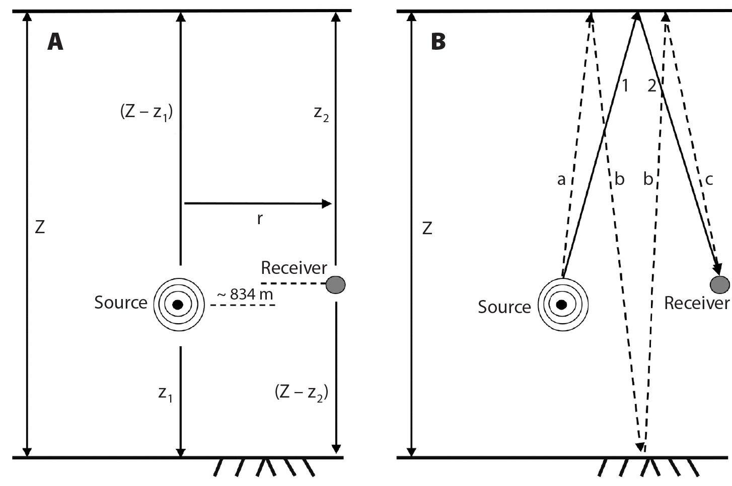
Figure 3. (A) The diagram of the paths taken by sound during the implosion and the variables describing those paths used in Equations 1–7, and (B) the diagram paths ps (solid line) and psbs (dashed line) accounting for the incident angle of the sound. > High res figure
|
The Paths Traveled by the Implosion Echoes
The implosion generated a very high amplitude, long pulse length, broadband pulse that was detectable even after multiple reflections from the seafloor and the surface (Figure 4a).
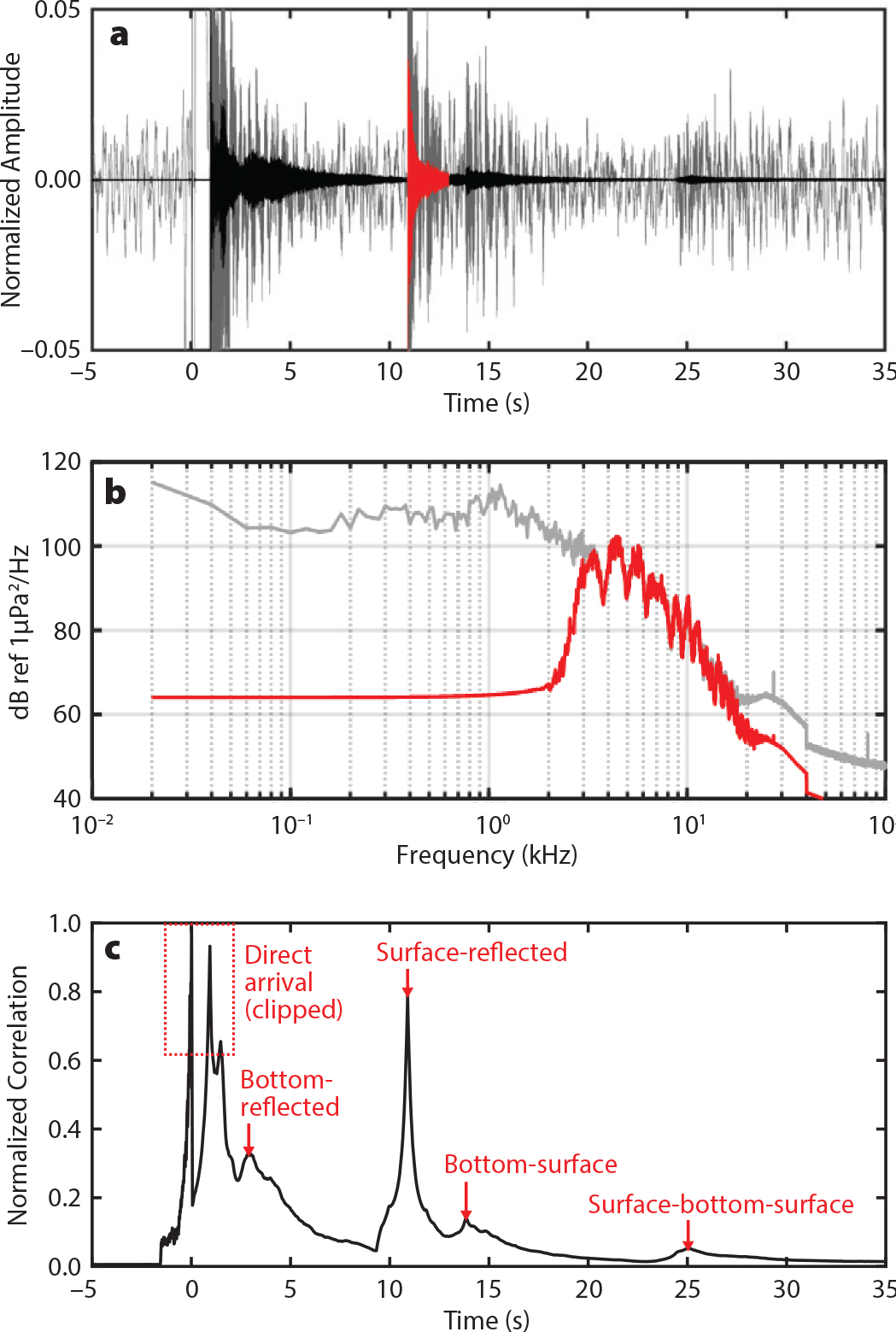
Figure 4. (a) The pressure time series recorded on Deep Sound Mk. II with the unfiltered raw signal (gray) and the band pass filtered signal (black), where the pseudo-transmit signal used in matched filter processing is highlighted (red). (b) The power spectra of the raw (gray) and band pass filtered pseudo-transmit signal (red), showing a pronounced peak and null structure in the pass band of the filtered signal. (c) The output of matched filter processing where the peaks in the correlation between the time series and the pseudo-transmit signal correspond to the arrival times of the shock wave as labeled. The mechanical saturation of the hydrophone and clipping during the digitization of the acoustic signal cause the direct arrival to appear as a group of three peaks in the matched filter output. > High res figure
|
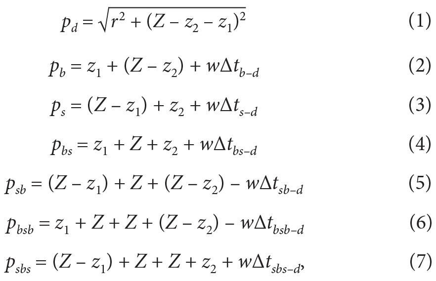
The paths traveled by the implosion pulse were: the direct path, pd, followed by the first bottom reflected path, pb, the first surface reflected path, ps, the bottom-surface reflected path, pbs, the surface-bottom reflected path, psb, the bottom-surface-bottom reflected path, pbsb, and finally the surface-bottom-surface reflected path, psbs. The paths are described by the following equations:
where Z is the unknown depth and w is the sinking rate of the receiver, 0.56 m s–1 with a standard deviation of 3 × 10⁻⁵ m s–1 over the time period of the recorded echoes. ∆tsbs–d is the difference in time between the arrival from path psbs and path pd.
Sound Speed Profile
The pressure, salinity, and temperature were recorded by Mk. II with a sampling rate of 1.83 Hz, corresponding to an average spatial resolution of 1.02 m, from the surface to its maximum deployment depth of 8,894 m. The sound speed was computed using both the Del Grosso equation (Del Grosso, 1974) and the TEOS-10 equation (IOC, SCOR, and IAPSO, 2010) for sound speed. The depth estimate resulting from the Del Grosso equation was 1 m shallower than that from the TEOS-10 equation, and therefore the more conservative estimate from the Del Grosso equation was chosen (Figure 5). More direct measurements of sound speed are needed at greater depths in trenches in order to evaluate the most appropriate model. CTD and sound velocity data collected during an earlier deployment in the Tonga Trench were used to compute the effective lags of each sensor on the CTD, either due to the mounting geometry of the probes with respect to the direction of motion or the characteristics of the probes themselves. The measurement uncertainty for each probe was reported by the manufacturer as 0.002°C for temperature, 0.0002 S m–1 for conductivity, and 0.02% for pressure. To predict the travel time for depths below 8,894 m, the sound speed profile was extended using a least-squares fit. Below 2,000 m, the sound speed profile is dominated by the increasing pressure and the relationship between depth and sound speed is well characterized. The sound speed profile from 2,000 m to 8,894 m was fitted with a second order polynomial (r2 > 0.9999, p < 0.0001), extending the profile to 12,000 m.
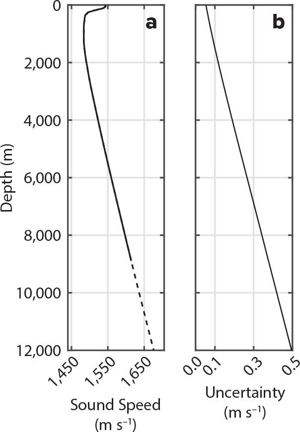
Figure 5. (a) The sound speed determined from measurements of temperature, salinity, and pressure from Deep Sound Mk. II and the Del Grosso (1974) equation, and (b) the uncertainty in the sound speed incorporating propagated measurement uncertainty and uncertainty in the Del Grosso equation (0.05 m s–1). > High res figure
|
Acoustic Signal Processing
Matched filter signal processing is a method used in radar and sonar systems to determine the time of arrival of an echo (see Turin, 1960; Lavery et al., 2010). A replica of the transmitted signal is correlated with the recorded time series, and maxima in the correlation are used to determine the arrival times of the reflected signal. Compared with the raw signal arrivals, the matched filter technique provides improved timing precision and higher processing gain. These performance metrics of matched filter processing improve with greater transmit signal bandwidth and frequency modulation (Chu and Stanton, 1998; Stanton and Chu, 2008; Lavery et al., 2010; Stanton et al., 2010). The distinct pattern generated by varying the instantaneous frequency is a poor match for Gaussian noise and deterministic signals with unrelated frequency content. In the case of this experiment, the implosion generated a highly energetic shock wave, which, although not frequency modulated, had a broad bandwidth spanning the entire frequency response band of the hydrophones. However, a distinct pattern of peaks and nulls in the frequency content of the implosion (Figure 4b) was sufficiently robust to permit the detection of echoes that traveled as far as the surface-bottom-surface reflected path, psbs. The direct-path arrival of the very high amplitude shock wave was clipped before saturating the hydrophones completely (Figure 4a time, t = 0–1 second), thereby precluding it as an effective timing reference. Accordingly, only the echoes from the surface and bottom boundaries were included in the matched-filter correlations.
Eleven seconds after the direct arrival, the surface-reflected echo arrived separated in time from the preceding and following echoes (Figure 4a). Showing a distinct peak and null structure in the frequency band from 3 kHz to 24 kHz (Figure 4b) and isolated in time from other arrivals, this segment of the time series was suitable for use as the template (transmit) signal in the matched filter processing. The time series and matched filter segment were filtered using a sixth order Butterworth filter with a pass band from 3 kHz to 24 kHz, highlighting the peak and null structure in the spectrum.
Identifying the Echoes in the Time Series
The output of the matched filter shows four discernible peaks, which, as shown in Figure 4c, may be identified as multipath arrivals. Preceding the first of these echoes, the three peaks labeled as “clipped” are associated with the direct-path arrival of the shock wave. As mentioned earlier, the distortion in this initial arrival renders it unsuitable as a precision timing tool, although it is adequate for providing a rough estimate of the travel times of the echoes.
To determine the likely path related to each peak, the travel time along each path was estimated and the arrival times were determined by computing tk, the discretely integrated time of flight
where ∆zi is the width of the depth bin and ci is measured sound speed at zi, I is the starting depth of integration, and K is the end depth. The depth bin size was constrained by vertical resolution of the measured sound speed profile, which was set by the sampling frequency of the CTD aboard Mk. II, as well as the instrument’s descent rate.
Using a nominal depth, Z, of 10,984 m, along with estimates of z1 and z2, it was possible to identify the four peaks in Figure 4c. The depth of the receiver, z2, was estimated to be 8,259 m at the time of the implosion, based on the CTD data and the pressure sensor on Mk. II using the Gibbs Sea Water package (IOC, SCOR, and IAPSO, 2010). Using the known descent rate of the source, 0.56 m s–1, and the time of the implosion, the depth of the source was estimated to be 9,093 m, (Z – z1). The time of the implosion was approximated by visually determining the time of arrival of the direct path at the receiver, and assuming the horizontal distance between the source and the receiver was 626 m, the same as the distance between their deployment locations.
Approximating the time of arrival for each echo revealed that the peaks in Figure 4c were the first bottom reflected echo, pb, the first surface reflected echo, ps, the bottom-surface reflected echo, pbs, and the surface-bottom-surface reflected echo, psbs. The surface-bottom reflected echo, psb, and the bottom-surface-bottom reflected echo, pbsb, were not detected.
The signal from pbs masked the signal from psb, which was estimated to arrive 0.27 s afterwards, while the pbs arrival was still active. However, pbs arrived first and was easily discerned from the ambient noise. The pbsb signal was the only pulse in the series that would have reflected off the seafloor twice and, assuming that the seafloor was a weaker scatterer than the sea surface, pbsb was likely to be masked by either psbs or the ambient noise. The fact that the surface return from ps at about 11 s in Figure 4a had a much higher amplitude than the other paths that reflect from the seafloor lends credence to the assumption that the seafloor was a weaker scatterer of sound compared to the surface.
The Depth of the Challenger Deep
Without knowledge of the exact time of the implosion (t0) or exact a priori knowledge of the length of pd, it is impossible to determine the absolute arrival time of any individual path. Therefore, analysis was restricted to evaluating the differences in arrival times among the four peaks. The only echoes necessary for determining Z were the surface-bottom-surface echo, psbs, and the first surface echo ps,
To determine the depth Z, Equation 8 was computed from the surface (i = 0) to the bottom (K = Z) while iteratively increasing K until tk was equal to the difference in the arrival times between psbs and ps, accounting for the distance traveled by the receiver array, w∆tsbs–b. Four estimates of Z were made by this method (one from the time series recorded on each of the four hydrophones), and it was found that Z = 10,980 m with a standard deviation of 5.0 m.
Accounting for Assumptions
Figure 3A and Equations 1–7 are simplifications of the paths traveled by the sound generated by the implosion. It was assumed that the ratio of the horizontal distance between Mk. II and Mk. III to the depth of Mk. II and Mk. III was sufficiently small to allow the paths to be approximated as being perpendicular to the sea surface and the seafloor. The actual paths traveled by the shock wave would each be the shortest path corresponding to a refracted ray at some angle determined by the sound speed profile gradient, the depths of Mk. II and Mk. III, and the horizontal distance between the probes. Figure 3B outlines a more realistic view of the paths traveled by the implosion pulse. In determining Z, it was assumed that differences between paths a and 1 and paths c and 2 were negligible. It was also assumed that the difference between Z and path b was negligible. It is possible to test these assumptions using nominal values for the depths of Mk. II and Mk. III and the distance between them. The difference between the slant range, line b in Figure 3B, and water depth Z was determined using nominal values for the depths of Mk. II and Mk. III (8,259 m and 9,093 m, respectively) and for the water depth (10,984 m). Using these nominal values and assuming that the source and receiver maintained a horizontal separation of 626 m, the difference between the slant range path and the vertical path (where r = 0) translates to a depth estimate difference of 3 m (see online supplementary materials). The estimate of Z in this study was accordingly increased by 3 m to 10,983 m to account for this potential path length difference.
While the potential error for the slant range correction for Z was only about 1 m, potential errors for reflections from the seafloor (z1 and Z – z2 in Figure 3A) due to uncertainties about the depth and, more importantly, the distance between the probes, were potentially more pronounced than for the first surface and later reflections. For these reflections, the ratio of horizontal distance between instruments to the range from the instruments to the seafloor was much larger, and the uncertainty in the horizontal distance made estimates of z1 and z2 obtained from paths pb and pbs uncertain.
Uncertainty Analysis
The uncertainty of the estimate of the depth of the Challenger Deep in this study came from two main sources: the uncertainty in measured arrival times from the hydrophone time series and the uncertainty in the modeled travel time. The modeled travel times rely on the empirical equation of state for seawater (IOC, SCOR, and IAPSO, 2010) and the Del Grosso equation (Del Grosso, 1974), from which the depth and sound speed can be computed from measurements made by the pressure, salinity, and temperature sensors, each of which has some associated uncertainty.
The sound speed profile was modeled according to Del Grosso (1974) using values measured by the pressure, salinity, and temperature probes. Del Grosso’s empirically derived relationship relies on regression fits to a library of previously collected data sets and describes their uncertainty as 0.05 m s–1. The depths of the sound speed profile measurements were determined using the TEOS-10 pressure-to-depth conversion equation that accounts for the dynamic height anomaly and the geopotential at zero pressure and has an error of less than 0.1 m (IOC, SCOR, and IAPSO, 2010). The uncertainties in the two models were combined with the instrument uncertainty to determine the complete propagated uncertainty in the modeled travel time (see online supplementary materials).
For the peak picking methodology, the uncertainty is assumed to be fully described by the standard deviation of the estimates of the travel times from the four hydrophones. The standard deviation between the estimates of the difference in arrival times between psbs and ps was 3.1 ms, which gives a difference in Z of 5.0 m.
The uncertainties in the peak picking methodology, the slant range calculation, and the modeled travel were combined to determine the total propagated uncertainty in the depth estimate. The total propagated uncertainty amounts to 3.5 ms, which corresponds to a depth uncertainty of ± 6 m (see online supplementary materials). Therefore, the estimate of the depth of Challenger Deep is 10,983 ± 6 m.
Discussion and Conclusion
The estimate of the depth of the Challenger Deep derived in this study, 10,983 ± 6 m, is among the deepest estimated depths (Figure 1a). The three other deepest measurements are by R/V Vityaz in 1957 (11,034 ± 50 m, revised to 10,983 ± 50 m by Taira et al., 2005), R/V Hakuho Maru in 1992 (10,965 ± 49 m), and the USNS Sumner in 2010 (10,984 ± 25 m). Among those measurements, this estimate is the most tightly constrained, with an uncertainty of ± 6 m. Factors that contributed to its low uncertainty include the concurrent and co-located CTD measurement of the sound speed profile made with modern temperature, salinity, and pressure probes with relatively low measurement uncertainties; precise measurement of reflected path arrivals, as permitted by the broad bandwidth of the implosion and multiple receivers; and low acoustic noise floor at the receivers. As Figure 1 shows, the estimate of the deepest part of the ocean has varied over time. Part of this variability can be accounted for by the differences in the positions of the estimates. The West Basin and East Basin are separated by approximately 50 km, over which the depth of the seafloor is likely to change.
A significant portion of the differences in depths can also be attributed to the variability in the methods used to make these estimates—not only the methods for generating the soundings (explosives, single- and multibeam sonars, pressure sensors, imploding instruments) but also the methods used to determine water column properties and the temporal lag between the water column property measurements and the soundings. Precise measures of sound speed and density throughout the water column are necessary for accurate soundings and for converting pressure measurements to depth. These differences in methods certainly explain some of the variability in the depth estimates. While the uncertainty in an individual measurement has improved, the uncertainty when comparing across measurements still raises questions as to the true depth of the deepest part of the ocean.
The accuracy of this estimate is limited by uncertainty in the time of arrival; the measurement uncertainty for the conductivity, temperature, and pressure probes; and the inexact underwater positioning information for the source and receiver. Additionally, the empirical equations used to compute the bulk properties of seawater, Del Grosso’s sound speed equation, and the TEOS-10 Gibbs seawater equations were not derived using data that faithfully represent seawater at pressures greater than 10,000 dbar and thus may introduce a systematic error that is difficult to quantify. The most significant source of uncertainty comes from the peak picking methodology. The arrival of the surface-bottom-surface reflection shows a much broader peak, especially when compared with the height, than the other reflections (Figure 4c). The smearing of the peak at this return is likely due to the large footprint of the acoustic wave by the time that it has traveled multiple water depths. The large footprint results in sound reflecting from uneven terrain at the seafloor and potentially from the walls of the Challenger Deep. Direct reflections off the seafloor, where the seafloor is perpendicular to the path of the sound wave, are higher in amplitude than reflections from terrain at other angles. The peak of the matched filtered signal represents the highest amplitude return from the surface-bottom-surface reflection. The peak of the surface-bottom-surface reflection was less pronounced and introduced significant uncertainty. In fact, the peak picking uncertainty is larger (3.1 ms) than the propagated uncertainty for the modeled time of flight, including the instrument uncertainty from the CTD measurements and model uncertainties (2.0 ms).
For acoustic measurements of depth, the uncertainty must account not only for the uncertainty in the time-of-flight measurement but also for both the uncertainty in the determination of the sound speed profile and any uncertainty due to differences in time between when the sounding is made and when the water column is profiled (Beaudoin et al., 2009). The concurrent measurements of water column properties and time-of-flight made by the Deep Sound platform do not suffer from such uncertainty.
Because depth computed directly from a pressure measurement is determined by integrating the water column above the pressure sensor accounting for the density, the uncertainties introduced by motion through the water column must be accounted for (Ullman and Hebert, 2014), such as the realignment of the conductivity and temperature probes based on sensor lag time (Horne and Toole, 1980; Gregg and Hess, 1985), the effects of viscous heating on the temperature probe (Larson and Pedersen, 1996), and the impact of the thermal mass of the submersible or instrument and CTD housing (Lueck, 1990). The Deep Sound platform has a relatively slow descent and ascent speed (0.56 m s–1), small thermal mass, and a CTD with a previously calibrated temperature and conductivity lag relationship.
The method used to determine the depth in this experiment relied on the implosion of an instrument at great depth. Similar results could be obtained by a broadband, frequency-modulated echo sounder deployed on a free-falling instrument. This instrument could ping as it descends through the water column while making simultaneous direct measurements of the sound speed. Sound speed equations and the equation-of-state of seawater are limited by a paucity of deepwater measurements for verification. Such an instrument would generate a large data set of many measurements of depth in a single dive, as well as provide much needed direct measurements of the sound speed in the ocean at great depths. Such an instrument could be deployed at Challenger Deep sites that have been indicated to be the deepest in order to more robustly estimate the depth and potentially settle the questions: how deep and where is the deepest part of the ocean?
Acknowledgments
The authors wish to thank the crew of R/V Falkor and the scientific team led by Douglas Bartlett during the 2014 expedition to the Mariana Trench. Dieter Bevans provided invaluable technical and field experience. Marina Antipina translated Russian language research papers about R/V Vityaz expeditions. An additional thank you to Andone Lavery of Woods Hole Oceanographic Institution. We would also like to thank three anonymous reviewers whose comments helped improve and clarify this manuscript. This work was funded by the Schmidt Ocean Institute, the Ocean Frontiers Institute, and the Office of Naval Research, Ocean Acoustics, Code 322OA, grant number N00014-18-1-2126.