Introduction
Frequent rainfall helps to maintain the relatively fresh (~33 psu) surface waters beneath the Intertropical Convergence Zone (ITCZ) of the eastern tropical Pacific Ocean. Rain cells on scales of O(1 to 100) km within the ITCZ episodically deposit freshwater onto the ocean surface, producing buoyant fresh layers that are eventually integrated into the underlying ocean through advection and mixing. One of the major objectives of the second Salinity Processes in the Upper-ocean Regional Study (SPURS-2) experiment is to understand the generation and evolution of rain-formed fresh layers, including the spatial and temporal scales of their salinity anomalies (defined in terms of the surface freshening observed by satellites). As part of the SPURS-2 experiment, we made measurements of temperature, salinity, and turbulent dissipation rate in the upper meter of the ocean at fine horizontal, vertical, and temporal resolution using the surface salinity profiler (SSP; Asher et al., 2014a,b), a surface-following platform that is towed from a ship. These data will enable us to characterize the structure of near-surface fresh layers formed by rain. In this article, we focus on the salinity response of the upper ocean to rain.
Although it is known that the strongest impact of rain occurs in the upper tens of centimeters of the ocean, few observations of salinity have been made over these shallow depths due to difficulties in sampling close to the ocean surface. Therefore, much of our detailed knowledge about the impacts of rainfall on the upper meter of the ocean comes from laboratory experiments (Ho et al., 2004; Zappa at al., 2009; Harrison et al., 2012) and modeling (Soloviev et al., 2015; Drushka et al., 2016; Bellenger et al., 2016). These studies have been supplemented by a limited number of field observations that have characterized rain impacts on the upper few meters of the ocean surface (e.g., Price et al., 1979; Soloviev and Lukas, 1997; Wijesekera et al., 1999; Asher et al., 2014a; Walesby et al., 2015; Moulin et al., 2018; Thompson et al., 2019; ten Doeschate et al., in press). The consistent results from these laboratory, modeling, and field studies indicate that rainfall forms layers of stably stratified fresher water on the order of 1 m to 10 m thick at the ocean surface, and that these “fresh layers” can persist from minutes to hours, depending on ocean surface mixing due to wind forcing, convective overturning, and internal and surface waves.
The impact of rainfall on the ocean is often characterized in terms of the vertical salinity gradient, ∆SZ2–Z1, between depths Z1 and Z2. As an example, salinity measurements from the Soil Moisture and Ocean Salinity (SMOS) or Aquarius satellite products, with a radiometric measurement depth of approximately 0.01 m, have been compared with salinity measured at 5 m by Argo profiling floats. The difference in salinity from these platforms gives ∆S5–0.01m, the vertical gradient in salinity between 0.01 m and 5 m depth. Several studies have determined that in the tropics there is a linear relationship between ∆S5–0.01m and the local rain rate (R):
∆S1.1–0.05m = kR, (1)
where ∆S5–0.01m > 0 indicates fresher values at 0.01 m compared to 5 m and R is provided by satellite-derived rain products (e.g., Boutin et al., 2014; Drucker and Riser, 2014; Santos-Garcia et al., 2014). Depending on the satellite data products used for salinity and rain, values for k ranging from 0.07 to 0.36 psu (mm hr–1)–1 have been estimated (see Boutin et al., 2016, for a review of these studies).
Equation 1 does not take into account other parameters that have been found to influence the formation of salinity gradients. For instance, wind can affect salinity gradients by generating turbulence that mixes the ocean surface (Asher et al., 2014a; Thompson et al., 2019; ten Doeschate et al., in press). Drushka et al. (2016) used a one-dimensional model to explore the influence of both rain rate and wind speed on vertical salinity gradients for idealized rain events having constant wind speed and a Gaussian-shaped rain rate time series. Similar to Equation 1, they found that
∆S5–0.05m = kRmaxU10–b, (2)
where U10 is the wind speed at a height of 10 m, Rmax is the maximum rain rate during the event, k = 0.11 psu (mm hr–1)–1, and b = 1.1. Equations 1 and 2 are not equivalent: for 2 ≤ U10 ≤ 10 m s–1 and 1 ≤ Rmax ≤ 100 mm hr–1, ∆S5–0.01m calculated using Equation 2 is an order of magnitude smaller than that predicted from fits of satellite/Argo data to Equation 1. The cause of this difference is unclear, but possible explanations are that a one-dimensional model may not fully account for all the processes governing fresh layer dynamics, or that differences in the spatiotemporal scales of satellite measurements (which are averaged in space and time) and the model (which represents a point measurement) could lead to the differences in the estimations of ∆S. There are also other factors not represented in Equation 2 that may be important for predicting vertical salinity gradients (e.g., preexisting surface ocean stratification, air-sea heat fluxes, mixing from surface and internal waves).
The objective of data collection with the SSP during SPURS-2 was to systematically characterize near-surface salinity, temperature, and turbulence within rain-formed fresh layers over a range of oceanic and atmospheric conditions. In this paper, we focus on the salinity and temperature measurements made from the SSP; detailed discussion of the microstructure turbulence measurements will be presented in a forthcoming study. The SSP measurements are used to quantify vertical salinity gradients within fresh layers, including their relationship to rain and wind forcing. The observations are also used to validate and reconcile the parameterizations in Equations 1 and 2.
Data
The Surface Salinity Profiler
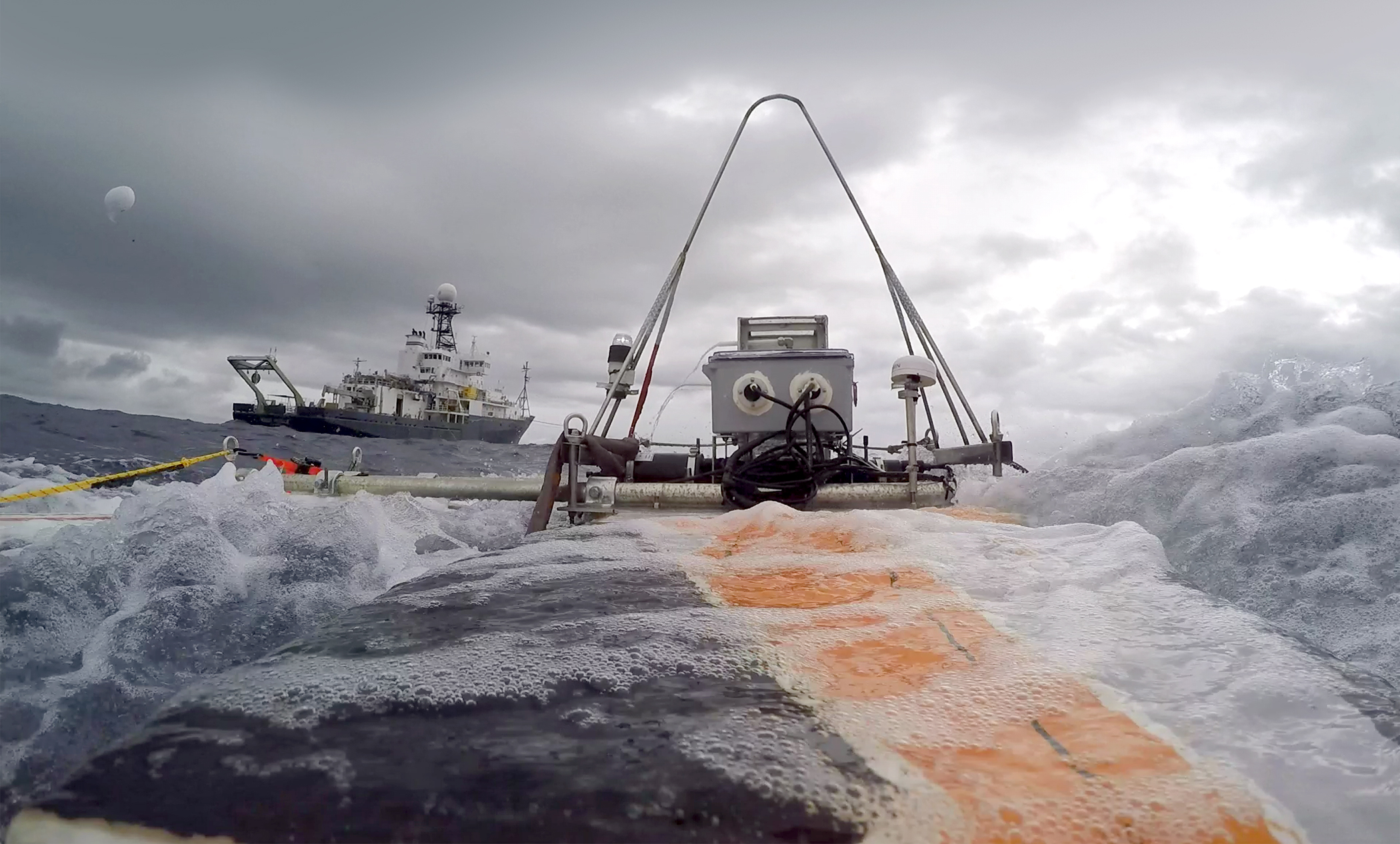
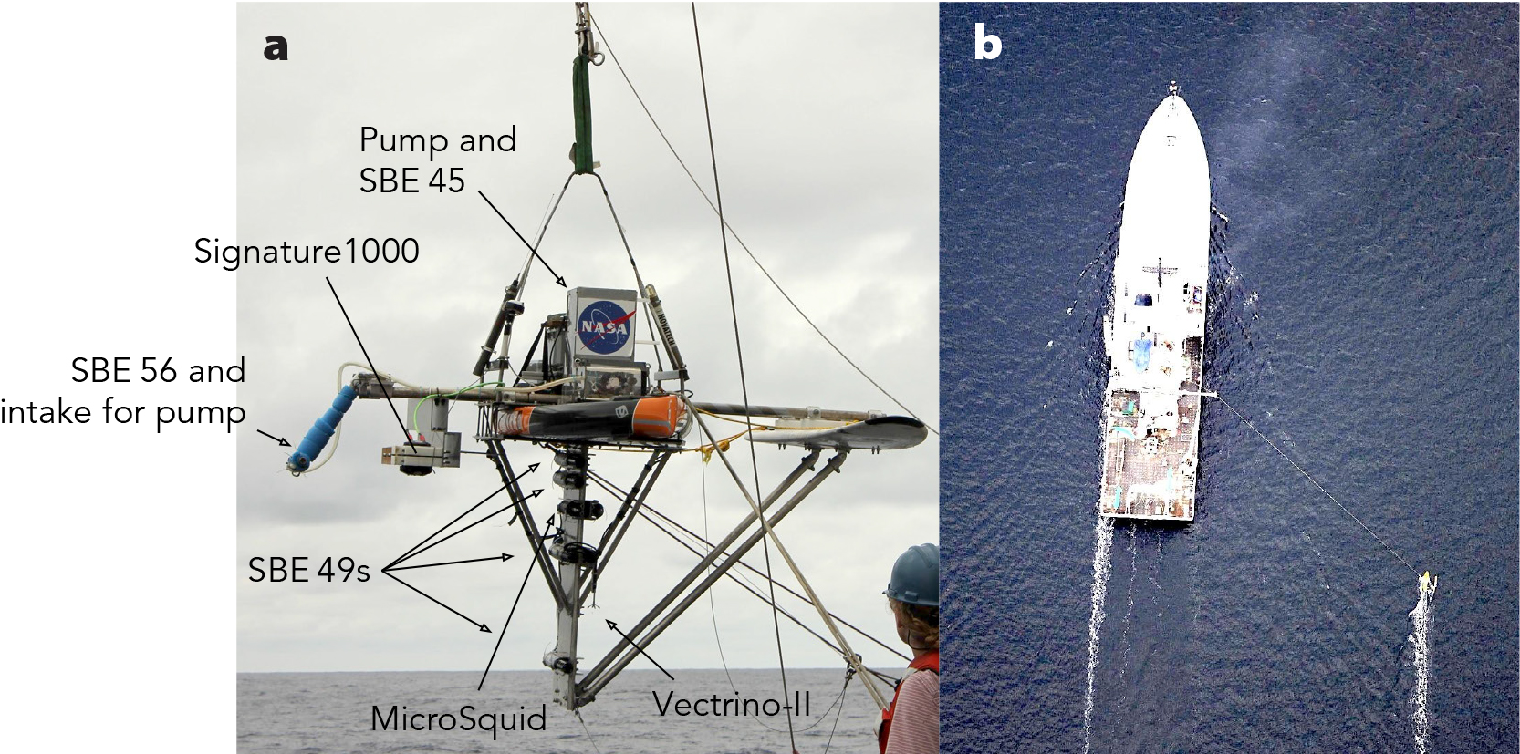
The SSP samples temperature and salinity in the upper meter of the ocean while being towed from a ship, as described by Asher et al. (2014a,b). The SSP used for SPURS-2 was a second-generation platform whose modified design provided additional capabilities. The modified SSP consisted of a 3.8 m long, 0.74 m wide, 0.13 m thick stand-up paddleboard attached with two horizontal struts to a 2.2 m long surfboard that was located inboard of the paddleboard relative to the ship. The paddleboard provided the majority of the buoyancy, while the surfboard acted as a stabilizing outrigger (Figure 1a). A 1.2 m deep by 0.6 m wide keel was affixed to the bottom of the center of the paddleboard and was secured to the outrigger with angled struts in order to reduce vibration of the instrumented keel and increase the strength of the SSP (Asher et al., 2014b). The keel of the SSP was constructed from a 12.5 mm thick layer of rubber sandwiched between 3 mm thick aluminum plates to further isolate sensors from vibration while the platform was towed.

Figure 1. Surface salinity profiler (SSP). (a) Front view of the SSP (2017 version) with instruments labeled. (b) Aerial view of SSP being towed from a research vessel (ship length is 84 m); note that the SSP is outside of the ship’s wake. In the 2016 deployments, the SSP did not include the Signature1000 or Vectrino-II, and the SBE 56 and pump intake were mounted to hoses that dragged in the water rather than on the sampling “arm” shown here. > High res figure
|
Four CTD sensors (SBE 49, Sea-Bird Electronics) were mounted to the keel at depths of 0.12, 0.23, 0.54, and 1.10 m below the ocean surface. Salinity in the upper 0.05 m was measured using a “salinity snake” that pumped water from a floating hose with an intake depth in the upper 0.05 m through a vortex debubbler and then a thermosalinograph (TSG; SBE 45, Sea-Bird Electronics). Seawater temperature at the intake of the salinity snake was measured using a self-logging temperature sensor (SBE 56, Sea-Bird Electronics) that was mounted on the intake hose (Figure 1a shows the articulated arm used for the 2017 field experiments that held the SBE 56 and intake hose for the salinity snake). Each CTD was sampled at 6 Hz, the TSG was sampled at 2 Hz, and the SBE 56 logged temperature at 1 Hz.
The SSP also measured the microstructure temperature and conductivity using probes (MicroSquid, Rockland Scientific) that were mounted to the SSP keel at 0.37 m depth below the water line. The microstructure probes were mounted on opposite sides of the keel, with each sensing element located forward of the CTD intakes in order to avoid flow distortion. In 2017, a downward-looking Nortek Vectrino-II profiling acoustic Doppler velocimeter (ADV) was mounted on the keel at 0.5 m depth and a downward-looking Nortek Signature1000 acoustic Doppler current profiler (ADCP) was mounted outboard of the paddleboard at a depth of 0.1 m. The ADCP operated in high-resolution mode and measured velocities in 0.02 m vertical bins from 0.2 m to 2 m depth below the sea surface. An inertial measurement unit took data that allowed platform motion to be decoupled from the ADV and ADCP velocity records.
The SSP was deployed episodically for up to 12 hours per deployment, with 18 deployments during the 2016 cruise and 16 during the 2017 cruise. During each deployment, the SSP provided a continuous record of temperature and salinity from 0.05 m to 1.1 m depth, along with measurements of turbulence from 0.2 m to 2 m. The SSP was towed from a point near the center of the ship on the port side using a 50 m long tow cable attached to a three-point bridle system, which forced it to track at a ~135° angle relative to the ship’s heading. As a result, the SSP was 35 m outboard and 10 m aft of the vessel, thus sampling water undisturbed by the ship’s wake (Figure 1b; Asher et al., 2014a,b). The SSP was towed at a maximum speed of 2 m s–1 in order to minimize bubble generation by the platform and to provide a reasonable balance between resolution of large- and small-scale horizontal features in the ocean. At this speed, the SSP followed the water level over swell and non-breaking wind waves such that the instruments maintained approximately the same depth below the sea surface. This was confirmed by the 0.02 m root-mean-square variance in the pressure data from the keel-mounted CTDs.
Salinity data from the CTDs mounted at 0.12 m and 0.23 m were processed to remove spikes (caused by bubbles) by computing a moving median and standard deviation over non-overlapping two- to five-minute data segments. The median salinity was subtracted from each data segment to isolate the salinity deviations, and data points in the original time series for which the corresponding value of the deviations were more than three times larger than the standard deviation were masked out. Missing data points were then filled either with linear interpolation if the missing value existed between two valid points or with a moving median of non-masked points taken from within the original segment of data. Salinity and temperature data at all depths were then smoothed with a 30-second moving median filter. Offsets and drift between each sensor were small, typically <0.001 psu for salinity and 0.008°C for temperature over the course of a 12-hour deployment. Mean differences in salinity and temperature between the CTDs, TSG, and SBE 56 were removed by selecting a time range for which the upper meter was well mixed (typically during night, or in non-rainy conditions with wind speed greater than 8 m s–1) and correcting mean values from all sensors to those of the CTD mounted at 0.54 m depth as a reference since it was shown to be the most stable sensor.
Other Observations
The upper-ocean measurements were complemented by a suite of ship-based measurements made continuously from R/V Revelle. These included rain rate and wind speed (Clayson et al., 2019, in this issue), water temperature and salinity from the ship’s TSG that sampled water from a nominal depth of 5 m, and ocean currents at 20 m depth and below from the ship’s ADCP (provided by Janet Sprintall, Scripps Institution of Oceanography). An Eigenbrodt ODM470 optical disdrometer was also deployed on the ship to measure raindrop size distributions. The meteorological sensors on the ship’s bow were approximately 90 m forward of the SSP’s position. At 2 m s–1 ship speed, this introduced a 45 s lag between the meteorological and SSP observations. All SSP measurements were thus offset by 45 s in time in order to account for this lag.
In this paper, we also use satellite-based rain estimates from IMERG (Integrated Multi-satellitE Retrievals for GPM, the NASA Global Precipitation Mission; Sun et al., 2018), which are available at 10 km horizontal resolution every 30 minutes.
Sampling Considerations
Sampling data from a moving platform in principle allowed us to capture the spatial structure of the response of the ocean to rain. However, the rain cells moved continuously (approximately with the atmospheric mean flow, which was typically faster than the ship speed) and evolved (on timescales as short as 60 s). Moreover, rainwater that was deposited on the ocean surface could then be advected horizontally by currents. Thus, the SSP observations represent the impact of the rain field, which moved and evolved, on the ocean surface, which also moved and evolved. The SSP measured the vertical distribution of salinity and temperature in a particular water parcel, and the ship measured the rain rate and wind speed that occurred over the parcel at the same time. However, the vertical temperature and salinity profiles of a given parcel also depended on the rain and wind speed history for that parcel, the details of which are not always known. As a result, correlating a salinity profile observed with the SSP to rain rates and wind speeds measured from the ship requires a cautious approach. Here, we assume that one-dimensional vertical processes (surface forcing, vertical mixing) dominated the oceanic response to rain forcing, so that over the timescales of the evolving rain field, the fresh layer evolved in the vertical direction faster than the lateral dispersion occurred. We also explore different metrics to describe rain forcing and predict the response of salinity to this forcing: the maximum rain rate of an event, the total accumulated rainfall during an event, and the instantaneous rain rate at any given time.
SSP Measurements of Near-Surface Salinity
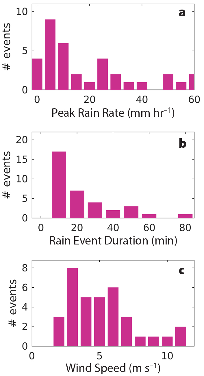
During the two SPURS-2 cruises, the SSP was deployed for a total of 230 hours, of which 39 hours were characterized as having local rain rates above 0.5 mm hr–1. Within those 39 hours, 35 distinct rain events were identifiable: 15 in 2016 and 20 in 2017. Here, we define a rain event as having (1) a rain rate, R, greater than 0.5 mm hr–1 for at least five minutes, and (2) a ∆S1.1–0.05m greater than 0.01 psu within ±15 minutes of the peak rain rate. The set of rain events spans a range of rain and wind conditions, with a median R of 11 mm hr–1 and a median duration of 27 minutes (Figure 2a,b). The associated wind speeds (adjusted to 10 m assuming neutral stability), U10, ranged from 2 m s–1 to 11 m s–1, with a median value of 5 m s–1 (Figure 2c). Although not shown here, R was not correlated with U10 so that the set of observed events allows investigation into how different rain and wind combinations affect the ocean salinity response to rainfall.

Figure 2. Statistics for the 35 rain events encountered while the SSP was deployed in 2016 and 2017. (a) Maximum rain rate during the events. (b) Duration of the events, defined as the total number of raining minutes. (c) Average wind speed during the raining minutes. > High res figure
|
Example Rain Event
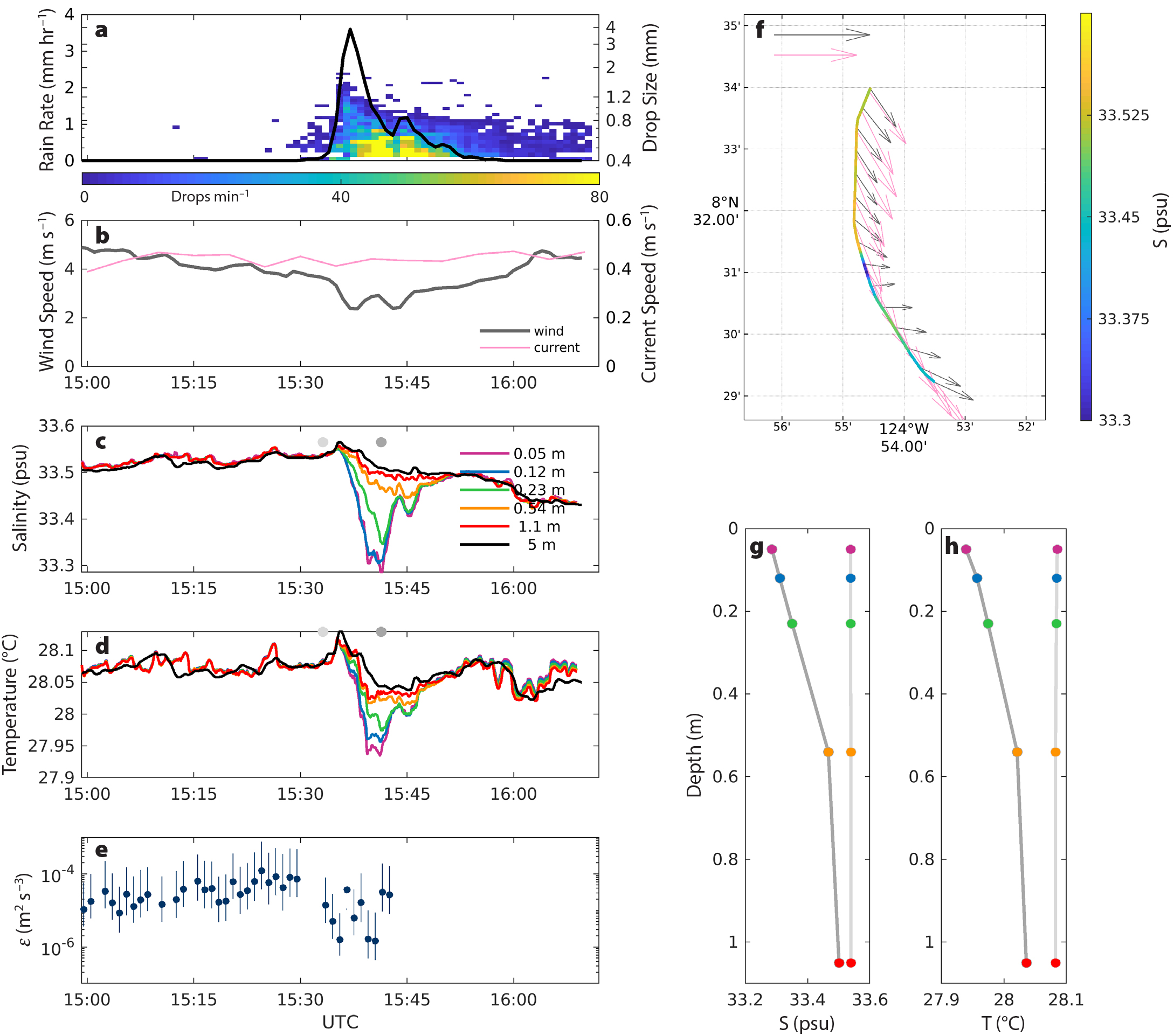
Figure 3 shows time series for R, rain-drop size distribution, U10, current speed at 20 m depth, salinity (S), temperature (T), and turbulent dissipation rate (ε)for one rain event sampled by the SSP. In this case, the SSP was being towed south-southwestward at 2 m s–1, and both the wind and current were from the north-northwest (Figure 3f). Before the rain began, the upper 5 m of the ocean were well mixed in temperature and salinity (Figure 3c,d). The rain event began at 15:33 UTC and had a maximum R, Rmax, of 4 mm hr–1 at 15:37 UTC. A smaller local peak in R of 1 mm hr–1 occurred at 15:45 UTC, and rain ceased at 15:58 UTC. The majority of raindrops had diameters less than 0.6 mm, and drops with diameter >1 mm were only observed when R > 1 mm hr–1 (i.e., when R was maximum for this event; Figure 3a). Wind speed dropped from 4.5 m s–1 to 2.3 m s–1, then increased again to 4.7 m s–1 after the time that Rmax occurred (Figure 3b).

Figure 3. Rain event sampled with the SSP on October 31, 2017. (a) Rain rate (black line, left axis) and number of drops of a given raindrop class size per minute (color, right axis) as measured by the disdrometer. (b) Wind speed (left axis) and current speed (right axis) measured from the ship. (c) Salinity and (d) temperature measured by the SSP and the ship’s thermosalinograph. (e) Dissipation rate at 0.37 m as derived from the microstructure conductivity sensor, with uncertainty bounds. (f) S0.05m (color) along the SSP track, with wind vectors (gray arrows; scale arrow at top is 10 m s–1) and current vectors (pink vectors; scale arrow is 0.5 m s–1). Vertical profiles of (g) salinity and (h) temperature from the SSP at 15:33 (light gray) and 15:41 (dark gray) UTC; these times are indicated as gray dots on panels c and d. > High res figure
|
The rain event generated freshening at all depths: the salinity anomaly followed the rain rate closely, with a lag of several minutes (Figure 3c). After the rain started at 15:33 UTC, S0.05m decreased by 0.27 psu from 15:35 to 15:41 UTC. At 15:41 UTC, four minutes after the time that Rmax occurred, S0.05m reached a minimum; immediately following this minimum, S0.05m increased by 0.16 psu. Following the second peak in R at 15:45 UTC, S0.05m decreased again by 0.04 psu, reaching a local minimum at 15:45 UTC (Figure 3c). From the time the rain started until 15:39 UTC, S0.05m and S0.12m were nearly equal, suggesting that the rainwater mixed instantaneously down to at least 0.12 m. This is consistent with laboratory experiments showing that turbulence generated by raindrops impacting on the surface penetrates to a depth of approximately 0.1 m and mixes this near-surface layer instantaneously (Zappa et al., 2009). Deeper than 0.12 m, the salinity anomalies were weaker and slightly lagged compared to S0.05m and S0.12m. For instance, S0.23m had a maximum decrease of 0.21 psu at 15:41 UTC, whereas S1.1m had a maximum decrease of 0.08 psu at 15:43 UTC. S5m measured by the ship’s TSG showed a maximum freshening of 0.07 psu at 15:51 UTC, indicating that the rainwater penetrated to at least 5 m depth (Figure 3c). After 15:54 UTC, a 0.07 psu freshening occurred at all depths. At this time, no local R was measured and no vertical S gradient was observed, suggesting that the fresh signal was measured when the SSP crossed a front. For instance, an earlier rain event could have caused freshening in that location and the subsequent mixing could have eroded the salinity stratification, leading to a horizontal salinity front but no vertical S gradient.
Figure 3d shows that T decreased in concert with the observed decrease in S at all depths. T0.05m decreased by 0.19°C between 15:35 and 15:41 UTC; T5m decreased by 0.08°C between 15:35 and 15:44 UTC. This rain-induced cooling is expected: the near-surface air is typically cooler than the ocean surface in the tropics, and raindrops are 1°–2°C cooler than the air (Gosnell et al., 1995), so raindrops tend to cool the ocean. As seen in salinity, T at all levels decreased again at 15:54 UTC, which is consistent with the SSP crossing a front.
The vertical profiles of S and T show that the maximum rain-induced freshening and cooling signals seen at 15:41 UTC were both strongest above 0.54 m (Figure 3g,h), indicating the formation of a thin (<0.54 m thick) stratified layer at the surface. Although measurements of ε are unavailable after 15:43 UTC, it appears that ε at 0.37 m decreased after the rain started, for example, at 15:41 UTC when the vertical stratification was strongest. It is possible that this reduction in turbulence occurred because kinetic energy from the wind stress was trapped within the stratified near-surface layer above the depth of the microstructure sensors.
Statistical Characterization of All Rain Events
The case study shown in Figure 3 is one example of the 35 rain events observed with the SSP during SPURS-2. To characterize all of the rain events and evaluate the parameterizations in Equations 1 and 2, several metrics have been defined. For each event, Rmax was identified as the peak rain rate, and the total amount of accumulated rainfall during each rain event, ΣR, was computed. RIMERG was estimated as the value of R from the IMERG satellite product within ±30 minutes of the time that Rmax occurred, in the pixel that the SSP was in. The strength of the rain-induced salinity anomaly was defined as the maximum value of ∆S1.1–0.05m within ±15 minutes of when Rmax occurred, and is referred to as ∆Smax. Similarly, ∆Tmax was defined as the maximum value of ∆T1.1–0.05m within ±15 minutes of the time that Rmax occurred. In order to capture the wind forcing affecting the development of ∆Smax,  was defined as the mean value of U10 over the time period spanning when Rmax and ∆Smax occurred. By definition, this time lag between Rmax and ∆Smax was <15 minutes; for the 35 rain events, it had a mean value of 3 minutes; that is, the peak vertical salinity gradient was generally observed within a few minutes of the peak rain rate.
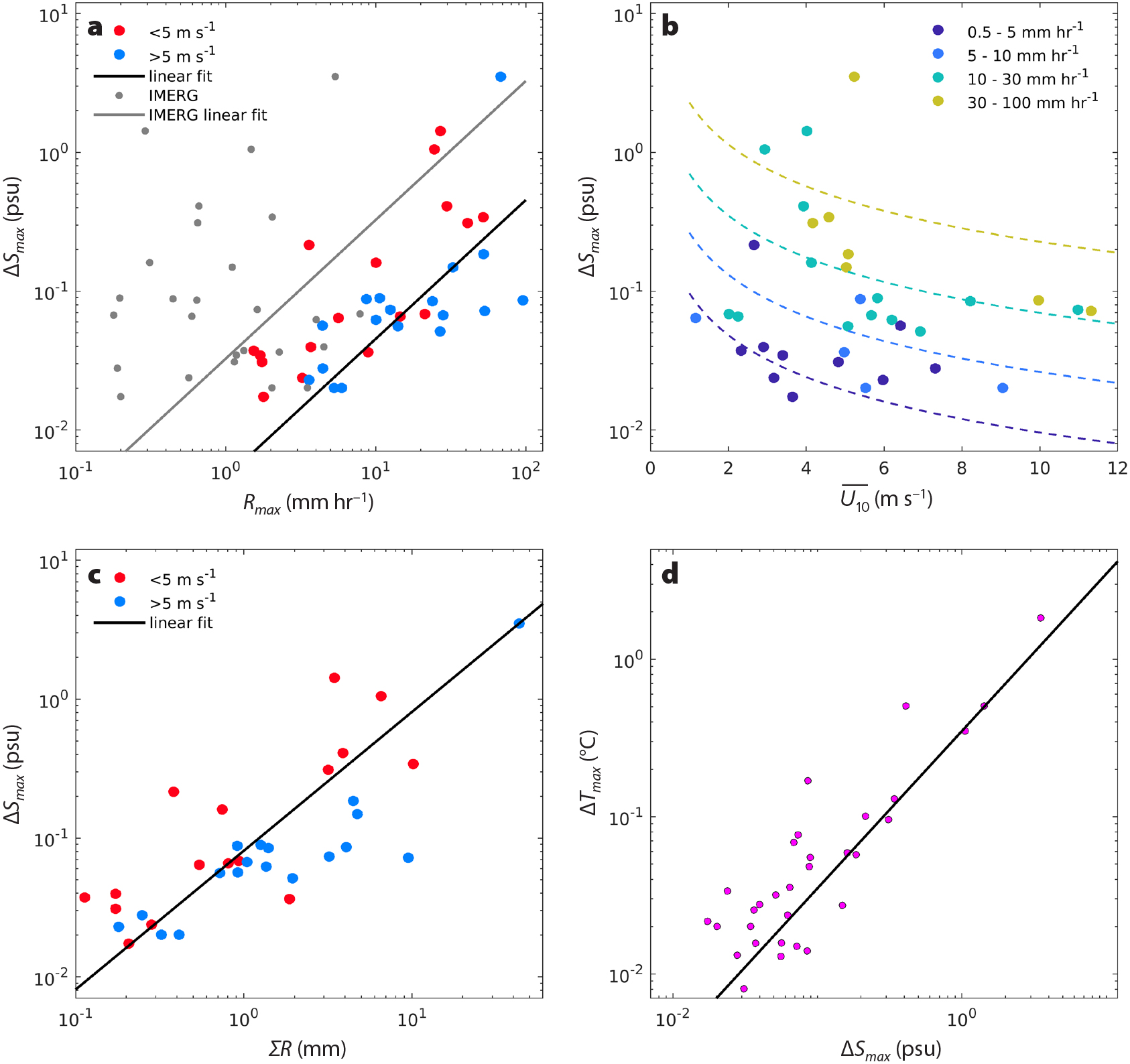
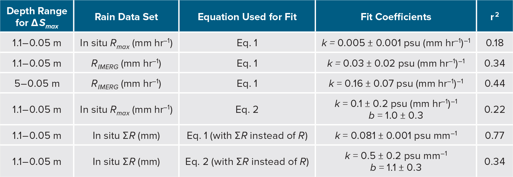
Figure 4 summarizes the various metrics used to quantify the rain, wind, and vertical salinity gradients for the rain events observed with the SSP. Least-squares linear regressions to Equations 1 and 2 were fit to these data in order to evaluate those relationships. Table 1 summarizes the results of the fits, and includes the coefficients and their standard errors as well as the coefficient of determination (r2) for each fit. Figure 4a shows a scatterplot of ∆Smax versus Rmax, where the points have been sorted into two classes based on wind speed:  > 5 m s–1 and
  ≤ 5 m s–1. Although considerable scatter exists in the data, it is evident that higher Rmax and lower
  are associated with larger ∆Smax. A least-squares linear regression between ∆Smax and Rmax (Equation 1) produced a regression coefficient of k = 0.005 psu (mm hr–1)–1 (Table 1). This value is over an order of magnitude smaller than the range of k shown in the review by Boutin et al. (2016) (from 0.07 to 0.36 psu (mm hr–1)–1). However, there are two major differences between the studies summarized by Boutin et al. (2016) and the present work: differences in measurement resolution and differences in the depths over which ∆S was calculated. First, the results shown by Boutin et al. (2016) were based on satellite-derived rain products, which have coarse resolution in space and time. The coarse satellite rain measurements have lower values than the in situ rain rates measured at the ship. This discrepancy is typical over tropical oceans where much of the precipitation falls from small-scale convective events with short duration and high intensity (e.g., Houze et al., 2015). Indeed, a scatterplot of ∆Smax versus RIMERG demonstrates that the values of RIMERG are an order of magnitude lower than the Rmax observed at approximately the same time and place (Figure 4a). The least-squares linear regression coefficient between ∆Smax and RIMERG is k = 0.03 psu (mm hr–1)–1 (Table 1), which is closer to the minimum value of k shown by Boutin et al. (2016) than the value of k estimated with in situ Rmax.

Figure 4. (a) ∆Smax plotted against Rmax for each event. Colored dots show ship-based rain measurements, colored by  . Gray dots show IMERG satellite-based rain measurements. The black and gray lines show linear fits to the ship-based and IMERG-based rain rates, respectively. (b) ∆Smax plotted against . Gray dots show IMERG satellite-based rain measurements. The black and gray lines show linear fits to the ship-based and IMERG-based rain rates, respectively. (b) ∆Smax plotted against  for each event, colored by Rmax. The thin dashed lines represent the fit of the data to Equation 2, evaluated at the midpoint value of Rmax in each rain rate range. (c) ∆Smax plotted against ΣR for each event, colored by for each event, colored by Rmax. The thin dashed lines represent the fit of the data to Equation 2, evaluated at the midpoint value of Rmax in each rain rate range. (c) ∆Smax plotted against ΣR for each event, colored by  . The black line shows a linear fit to the data. (d) ∆Tmax plotted against ∆Smax for each event. The black line shows a linear fit to the data. > High res figure . The black line shows a linear fit to the data. (d) ∆Tmax plotted against ∆Smax for each event. The black line shows a linear fit to the data. > High res figure
|
Table 1. Parameters used in fitting observations to Equations 1 and 2, and resulting coefficients. > High res table

|
Second, Boutin et al. (2016) considered ΔS5–0.05m, while this study considers ΔS1.1–0.05m. Although not plotted here, the regression of ΔSmax to RIMERG, where ΔSmax was computed from ∆S5–0.05m (with S5m measured by the ship’s TSG), produced a coefficient k = 0.16 psu (mm hr–1)–1 (Table 1), which is consistent with the results presented by Boutin et al. (2016). In other words, the measurements of individual fresh layers made during SPURS-2 show a relationship between rain rate and vertical salinity gradient that is consistent with relationships developed with satellite-based measurements.
While Equation 1 assumes that ∆Smax depends only on Rmax, Equation 2 describes ∆Smax as a function of both Rmax and  . It is evident from the SSP data that ∆Smax depends on both Rmax and
  (Figure 4b). Although these data exhibit significant variability, they demonstrate that the highest values of ∆Smax occur during rain events with higher Rmax and smaller
  . A fit of Equation 2 to the data in Figure 4a,b gives values of k = 0.1 ± 0.2 psu (mm hr–1)–1 and b = 1.0 ± 0.3 (Table 1). This fit is shown as dashed lines in Figure 4b. Though the uncertainty bounds (standard errors) of these coefficients are wide, the values are consistent with those found by Drushka et al. (2016) using output from one-dimensional modeling of idealized rain events. This suggests that although the rain events simulated with the one-dimensional model by Drushka et al. (2016) were idealized in terms of the temporal evolution of R and U10, the modeled dependence of ∆Smax on Rmax and
  is similar to that found with field observations. This confirms that it is reasonable to use one-dimensional models to investigate the effect of rainfall on near-surface salinity.
Although the regression coefficients from fitting field data to Equation 2 are consistent with those found by Drushka et el. (2016), the scatter in Figure 4b suggests that factors other than Rmax and  likely have significant impacts on ∆Smax. For instance, detailed inspection of the individual rain events captured with the SSP on a case-by-case basis reveals that the development of ∆S appears to be affected by horizontal advection in the upper ocean (current speeds were on average 0.3 m s–1) and preexisting stratification from either diurnal warm layers or rain-generated fresh layers from previous rain events.
To evaluate the ability of accumulated rainfall to describe the strength of rain-formed vertical salinity gradients, Figure 4c shows ∆Smax plotted against ΣR. The r2 value for the linear regression between ∆Smax and ΣR (i.e., replacing Rmax with ΣR in Equation 1) is 0.77. This r2 value is much larger than that for the fit between ∆Smax and Rmax (r2 = 0.18; Table 1), which indicates that ΣR is a better predictor of ∆Smax than Rmax is. The fit between ∆Smax and ΣR using Equation 1 is also better than the fit of ∆Smax to ΣR and  using Equation 2, which has an r2 value of 0.34 (Table 1). In other words, variability in ∆Smax can mostly be explained by variability in ΣR without considering U10. This finding is counter-intuitive in light of the wind dependence that is seen in Figure 4a,b. We hypothesize that the variability of wind speed over the course of a rain event generates a time-variable and nonlinear forcing due to vertical mixing that is not well represented by an average value of wind speed. Thus, fitting ∆Smax to ΣR and
  (Equation 2) degrades the fits in comparison to fitting ∆Smax only to ΣR (Equation 1). Alternatively, it may be that Equation 2 is not the correct model for the wind dependence of ∆Smax.
The close correlation between salinity and temperature variations during rain events (Figure 3c,d) was observed during all 35 rain events observed with the SSP. This is illustrated in Figure 4d, which shows a high correlation between ∆Tmax and ∆Smax. A least-squares linear regression using data from the 35 events produces the relationship ∆Tmax = (0.35 ± 0.01°C psu–1) ∆Smax, and has an r2 value of 0.89. This strong linear relationship is consistent with results from the prognostic model that was developed by Bellenger et al. (2016) to represent rain freshening and cooling.
Instantaneous Response of Upper-Ocean Salinity to Rain and Wind
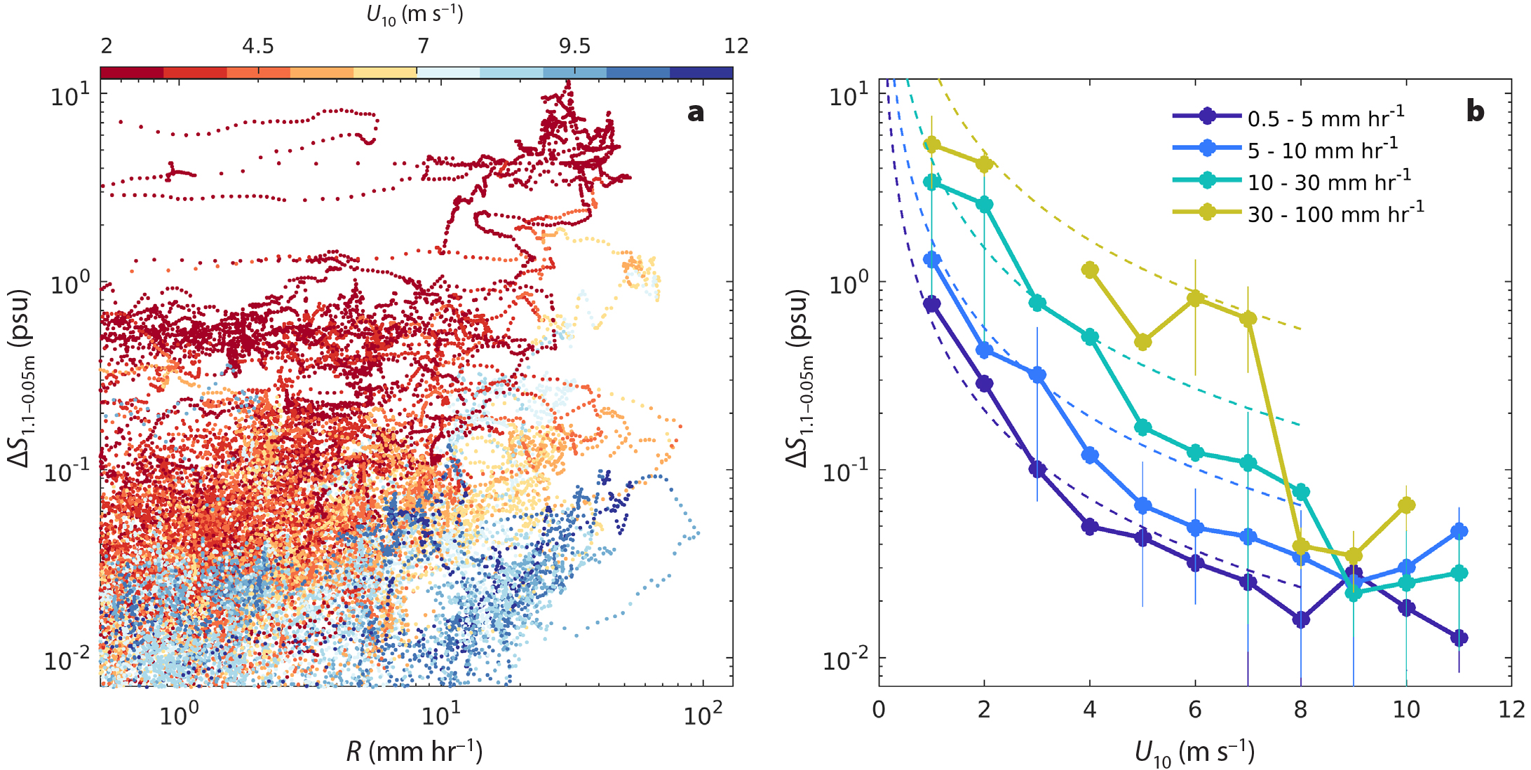
In the two sections immediately above, individual rain events were isolated and quantified using ∆Smax and Rmax. It is also useful to quantify the instantaneous relationship of ∆S with R and U10 at any given time. An instantaneous relationship may be particularly applicable to satellite data, which represent snapshots (e.g., of R, U10, or S0.01m) and thus may not capture the maximum R or minimum S0.01m for a given rain event. Here, we relate ∆S to R and U10 for all times that it was raining, without separating the data into discrete rain events. Figure 5a shows ∆S1.1–0.05m for all data points having R > 0.5 mm hr–1 as a function of R, where the data point color denotes U10. The dependence of ∆S1.1–0.05m on both R and U10 is clear: ∆S1.1–0.05m is positively correlated with R, with the largest ∆S1.1–0.05m observed when U10 is low. This can be seen by binning ∆S1.1–0.05m as a function of U10 and R (Figure 5b), which shows a clear correlation of ∆S1.1–0.05m with R and U10 when U10 < 7 m s–1. At higher wind speeds, ∆S1.1–0.05m is small and no longer shows a dependence on R, suggesting that salinity gradients in the upper meter of the ocean are rarely seen for wind speeds greater than about 7 m s–1 (consistent with the observations of Thompson et al., 2019). Figure 5b demonstrates that the average salinity response in the upper 1 m of the ocean to rainfall is effectively instantaneous, with local rain and wind explaining much of the variability in ∆S1.1–0.05m. A fit of Equation 2 to all of the data shown in Figure 5a for U10 < 8 m s–1 gives the coefficients k = 0.21 ± 0.01 (mm hr–1)–1 and b = 1.54 ± 0.01 (shown as thin dashed lines on Figure 5b). Thus, ∆S1.1–0.05m observed by the SSP is linearly related to R and inversely proportional to U10 at any given time, consistent with ∆Smax for individual rain events (Figure 4b) and ∆S estimated with a one-dimensional model of idealized rain events (Drushka et al., 2016).

Figure 5. (a) ∆S1.1–0.05m as a function of R for all data collected with the SSP while R > 0.5 mm hr–1, where each data point has been colored by U10. (b) ∆S1.1–0.05m as a function of U10, colored by R. Dots and thick lines represent the raw data shown in Figure 4a that have been binned by R and U10. Thin dashed lines represent fit of Equation 2 to all raw data having U10 < 8 m s–1, which gives ∆S1.1–0.05m = 0.22 ⋅ R ⋅ U10–1.6, evaluated at the midpoint value of R in each rain rate range. > High res figure
|
Discussion and Conclusions
During the 2016 and 2017 SPURS-2 cruises, the SSP measured vertical profiles of temperature and salinity from 0.05 m to 1.1 m and dissipation rate at 0.37 m depth for 35 distinct rain events. These events represent 39 hours of data collected during a range of wind and rain conditions (Figure 2). The SSP measurements produced a rich data set that enables detailed characterization of the response of the upper meter of the ocean to rainfall. A major focus of this paper was to assess two parameterizations that have been developed to describe the vertical salinity gradients that form due to rainfall (Equations 1 and 2).
Equation 1 is a linear relationship between ∆Smax and Rmax that was developed using satellite-based rain products and satellite/Argo salinities (Boutin et al., 2014, 2016). In situ rain rates measured from the ship were an order of magnitude greater than satellite-based rain rates from the IMERG product (Figure 4a). When this difference in R between IMERG and in situ is accounted for, and the depth range over which ∆Smax is computed is taken into account, the SSP-based regression coefficient between ∆Smax and Rmax is in agreement with the results presented by Boutin et al. (2016). This result implies that applying or comparing parameterizations of near-surface salinity stratification due to rainfall requires careful consideration of the spatial and temporal scales used.
Fitting Equation 2 using Rmax and  to the ∆Smax (Figure 4b) produced coefficients that, within the uncertainties, were consistent with the results from a one-dimensional modeling study of idealized rain events (Drushka et al., 2016). This agreement suggests that although the idealized rain events in the model oversimplified the atmospheric forcing on the ocean, the modeled response of the upper ocean to rainfall and wind compares reasonably well to that observed with the SSP. However, wide scatter in the data and large uncertainties on the fit to Equation 2 indicate that ∆Smax is not well described with a simple parameterization based on Rmax and
  . Other factors, such as mixing from surface and internal waves, advection, and existing near-surface stratification also likely affect the vertical salinity gradients generated by rain. In addition, as described in the section on Sampling Considerations, sampling a constantly evolving rain field from a moving platform also likely confounds the temporal and spatial variability of the impact of rainfall on ∆S. It is thus unsurprising that ∆Smax cannot be perfectly described by Rmax and
  .
.
Equations 1 and 2 were both developed using rain rate as a metric to describe ∆Smax. The data shown in Figure 4c demonstrate that the total accumulated rainfall for an event (ΣR) describes the strength of vertical salinity gradients better than the peak rain rate of an event (Table 1). This finding is in contrast to the results of the modeling study of Drushka et al. (2016), who found Rmax to be a better predictor of ∆Smax than ΣR. This can be explained by the fact that the idealized rain events modeled by Drushka et al. (2016) were forced using constant U10 and a smooth time series of R with a single peak. Those forcing characteristics led the model to predict a single well-defined ∆Smax for each rain event. The situation is rarely so simple for real-world rain events, in which rainfall intensity varies on short timescales and small spatial scales. Rain accumulation thus explains more variability in ∆Smax than does Rmax. Interestingly, regressing ∆Smax to ΣR alone produces a much better fit in comparison to including  in the fit, despite the clear dependence of ∆S on both wind speed and rain rate demonstrated in Figures 4b and 5b. We speculate that because wind speed varies significantly during the course of a single rain event, an average value of wind speed does not represent the nonlinear impacts of wind forcing on upper-ocean mixing and hence on ∆S. Including
  thus degrades the fit of Smax to ΣR. In addition, Equation 2 may not be the best model to describe the wind speed and rain dependence of vertical salinity gradients. Unraveling the relative effects of time-variable rain, wind, and mixing on vertical salinity anomalies is beyond the scope of this paper and is left to future studies that combine modeling and analysis of the SSP data collected during SPURS-2.
By considering ∆S at any time as an instantaneous salinity response to local wind and rain forcing, Figure 5b demonstrates that ∆S is linearly related to R and inversely related to U10 (for U10 < 8 m s–1). This is potentially valuable for using instantaneous measurement of R and U10 (e.g., from satellites or infrequent in situ measurements) to predict the presence of near-surface salinity stratification. The very high correlation between ∆Tmax and ∆Smax (Figure 4d) has potential implications for using temperature as a proxy for salinity in order to study near-surface fresh layers. Near-surface temperature measurements (e.g., from satellites and surface drifters) are more prevalent than near-surface salinity measurements. If rain-induced cooling can be identified from temperature observations, and distinguished from cooling due to other causes (e.g., by matching to satellite rain observations), it may be possible to estimate rain-induced ∆S from ∆T measurements.

