The high-latitude Pacific is home to highly productive ecosystems, including vast populations of commercially and subsistence harvested fish. These regions can be challenging to sample directly. Over several decades at the NOAA Pacific Marine Environmental Laboratory, we have applied numerical models to infer past, present, and future states of these regional oceans and their biota. These estimates are provided to fisheries scientists to help identify the local biophysical dynamics that underlie marine resource fluctuations and to managers to help develop effective management strategies in the face of short- and long-term environmental changes.

Daily average surface chlorophyll concentration (July 21, 2001) from a biogeochemical model of the Gulf of Alaska (blue = lowest concentration, red = highest), with bathymetry superimposed. > High res figure

Introduction

This article provides an overview of biophysical modeling efforts at the NOAA Pacific Marine Environmental Laboratory (PMEL) centered on the high-​latitude North Pacific. Over the past four decades, these efforts have been guided by observations and motivated equally by unknowns in fisheries oceanography and societal needs for effective ecosystem management. As an example, modeling for the Gulf of Alaska (GOA), carried out under the PMEL Fisheries Oceanography Coordinated Investigations (FOCI and successor EcoFOCI) program, was motivated by observations of a surge in the populations of spawning walleye pollock (Theragra chalcogramma) in Shelikof Strait in the early 1980s (Figure 1 in Mordy et al., 2023, in this issue). The complex bathymetry and hydrodynamics of the Shelikof Strait region limited the suitability of simple analytical models and required a numerical modeling framework capable of resolving regional topography and fine vertical structure through the water column. At the time, the Semi-spectral Primitive Equation Model (SPEM), developed primarily at Rutgers University (Haidvogel et al., 1991), was a logical choice for this purpose (Hermann and Stabeno, 1996). SPEM was used to model the physics of this complex region and test several hypotheses regarding physical drivers (e.g., changes in advection and ocean temperature) for the walleye pollock shift. Over time, this focus expanded to include the wider GOA and the Bering and Chukchi Seas as well as testing of a much larger set of hypotheses in fisheries oceanography. Subjects of these hypotheses include, but are not limited to, the roles of larval advection, match/​mismatch of larvae with prey density (Doyle et al., 2019), drivers of high primary production in the coastal GOA where downwelling circulation predominates (Coyle et al., 2019), and the impacts of seasonal sea ice on production in the Bering Sea (e.g., the “Oscillating Control” hypothesis; Hunt et al., 2011).

A central goal of these efforts is to capture the realistic dynamics of the fluid using hydrodynamic models that are constructed following the laws of physics governing ocean circulation and changes in water mass properties. The models are driven at the sea surface by atmospheric forcing and at the lateral boundaries for limited domain modeling by input from the surrounding oceans and terrestrial runoff. The development of accurate lateral boundary conditions for ocean hydrodynamics and biogeochemistry has been, and continues to be, a significant challenge to the successful modeling of regional oceans.

The hydrodynamic models we use have evolved over the years. The numerical structure of SPEM did not allow for a tidally varying sea surface height and hence proper tidal mixing and circulation, a major feature of the region. SPEM did, however, resolve small-scale (30 km) eddies and other prominent features of the Alaska Coastal Current (Figure 1). A successor to this code, the S-Coordinate Rutgers University Model (SCRUM; Song and Haidvogel, 1994), did allow for a free ocean surface, and hence was used to implement nested regional models of the GOA and the Bering Sea that included tidal forcing. Both SPEM and SCRUM were based on terrain-​following vertical coordinates, which helped to resolve vertical structure over the irregular topography of our regions. Ultimately, developers at Rutgers and UCLA produced the Regional Ocean Modeling System (ROMS; Haidvogel et al., 2008), which included the desirable properties of (1) a free sea surface, (2) an efficient representation of vertical structure, and notably, (3) built-in options for data assimilation. Most significantly for our Bering Sea work, ROMS was enhanced to include ice dynamics and thermodynamics (Danielson et al., 2011). The work at PMEL benefited from each of these models, and many hard-won recommendations from collaborators on best parameter choices and procedures for developing regional boundary conditions. More recently, the NOAA Geophysical Fluid Dynamics Laboratory’s open-​development Modular Ocean Model version 6 (MOM6; Adcroft et al., 2019) has played a growing role across NOAA, including at PMEL. While MOM6 was initially applied in global configurations, it is now implemented in several regional configurations that include Northeast Pacific and Arctic domains. It includes a flexible vertical coordinate system that permits a range of strategies for resolving shelf-scale features, including steep bathymetry, while also maintaining off-shore water masses. It also includes flexible time-​stepping options that allow for faster execution of the code when incorporating many state variables (as in biology-​focused configurations). Ultimately, this could allow for longer simulations, larger predictive ensembles, and finer spatial resolution than would be affordable using earlier codes.

 

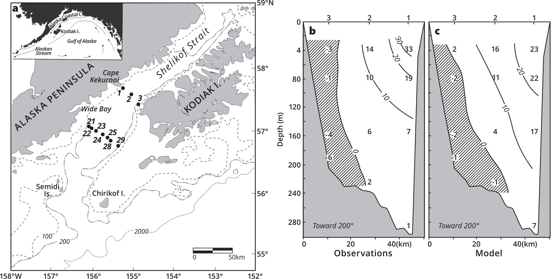
FIGURE 1. An early comparison of moored current meter data and the Semi-spectral Primitive Equation Model (SPEM) for the northern Gulf of Alaska (a, with moorings numbered) illustrates observed (b) and modeled (c) velocities (cm s–1) off Cape Kekurnoi using data from moorings 1–3. From Stabeno and Hermann (1996). > High res figure

 

These hydrodynamic models are coupled with ocean biogeochemistry modules to study biophysical interactions. Over the years, we have been fortunate to work with a wide multidisciplinary cast of colleagues, including research units within PMEL, the Alaska Fisheries Science Center (AFSC), the University of Alaska Fairbanks, and Rutgers University. These collaborations have striven to elucidate the mechanisms connecting physics and biogeochemistry to the population dynamics, movement, and reproduction of managed species in a region of the world that is difficult to sample directly. Collectively, we have recognized the virtue (and challenge) of combining multiple elements within a single model, allowing for both “bottom-up” and “top-down” dynamics to guide the emergent model behavior. For example, some allowance for fish and mammals to impact the populations on which they feed is included (e.g., Ortiz et al., 2016). In practice, this coupling is quite difficult, not only because of the sparse observations available to constrain the form and parameterization of the key processes but also because of the sheer number of desired state variables (many different species and life stages) and the computational demands this entails.

The coastal subarctic regions of the GOA and the Bering Sea present some unique challenges to simulating biogeochemistry: wide, shallow shelves supporting diverse mesozooplankton populations and large benthic communities; the presence of sea ice and ice-​associated plankton and algae; and substantial land-based input of nutrients like iron (Coyle et al., 2019). Because of these conditions, a number of custom biogeochemical (i.e., nutrient-​phytoplankton-​zooplankton, or NPZ) models have been developed for the region, development that must continually balance the desire to simulate the complexity that has been hypothesized as essential for success with the limited amount of observational data available to validate and parameterize such complexity. Our high-​latitude NPZ models initially included only a few nutrient, phytoplankton, and zooplankton groups (Figure 2), but they have since been expanded to include multiple nutrient currencies (including carbonate system dynamics), multiple phytoplankton and zooplankton functional groups (Pilcher et al., 2019; Kearney et al., 2020), and benthic and ice biogeochemistry modules. Computational and file storage constraints must also be considered as models grow to include more state variables, resolve smaller-scale processes, cover longer time periods, and use larger ensembles to quantify uncertainty. Advances in computing may help to alleviate some of these limitations, allowing for larger ensembles to explore a larger volume of parameter space, and hence better quantify the uncertainty of any biological predictions and projections.

 

FIGURE 2. (a) Schematic of an early use of a hydrodynamic model (SPEM) with a lower trophic level model. Modified from Hinckley et al. (2009). (b) Flowchart of hydrodynamic model forcing, nesting, comparisons with data, and linkage with biological models. Modified from unpublished GLOBEC flowchart by E.L. Dobbins, University of Alaska Fairbanks. > High res figure

 

In classical Eulerian (fixed-grid) NPZ, fish, and marine mammal models, we track the average properties of a population within each model grid cell, neglecting the variation among individuals within that grid cell. An alternative approach treats fish and mammals as individuals subject to both advection and self-directed motion. One great motivator for this individual-based approach is the classic dictum (historically attributed to Gary Sharp) that “the average fish is dead”—that is, only a fortunate few survive to adulthood, and we should focus on what makes them successful, rather than on the average (hence unsuccessful) individual. Given the strong natural dispersion (mixing) of the marine environment, this approach requires a large initial population, along with “reseeding” of individuals where they become sparse. With biological colleagues, we ultimately implemented this Individual-Based Modeling method using SPEM and ROMS, both online (as part of the execution of the hydrodynamic model) and offline (using stored hydrodynamic output; e.g., Gibson et al., 2022).

 

Modeling Highlights and Integration of Modeling and Observations

In this section we highlight a few regional downscaling activities using the models and approaches introduced above. Our modeling domains have spanned the Northeast Pacific, from the Washington coast (Siedlecki et al., 2023, in this issue) to the GOA (Gibson et al., 2022) and the Bering Sea (Cheng et al., 2021; Hermann et al., 2021). Many of these multidisciplinary models were developed in conjunction with large field campaigns (e.g., the Bering Sea Project). The lengths of the simulations range from seasonal to multidecadal. In general, the modeling types can be divided into: (1) retrospective hindcasts where simulations are forced by past ocean and atmospheric conditions and therefore can be directly compared with observations; (2) seasonal forecasts where the regional ocean is initialized by present “known” (observed or estimated) conditions and run forward in time for 9–12 months, driven by global predictions from operational weather forecast and research centers; and (3) multidecadal projections where the regional ocean is forced by ocean-​atmosphere conditions as simulated by global Earth System Models (ESMs) under greenhouse gas and aerosol forcing scenarios (IPCC reports; see Drenkard et al., 2021, for overview). We also discuss the importance of integration between modeling and observations.

 

Retrospective Hindcasts

Hindcasts—simulations of past conditions—​have long been used in physical oceanography to identify the primary mechanisms driving observed ocean change (e.g., El Niño-Southern Oscillation). Many of the products resulting from our (PMEL and AFSC) modeling efforts have been directed at users within the fisheries community. A fundamental question addressed by EcoFOCI has been the fate of spawned fish larvae—where do they go and how do some larvae become more successful than others? Hindcast simulations evaluated against historical observations allow us to address dynamical linkages among the ocean biophysical environment, ecosystem responses, and fisheries management. Major enhancements to our retrospective biophysical modeling capabilities were achieved through collaborations with large interdisciplinary programs such as the Global Ecology Program (GLOBEC; Curchitser et al., 2013), the Gulf of Alaska Integrated Ecosystem Research Program (GOAIERP; Gibson et al., 2022) and the Bering Sea Program (BEST-BSIERP; Hunt et al., 2011). The GLOBEC work included an elaboration of our NPZ components to include multiple size classes of plankton and highlighted the importance of iron in runoff influencing production on the GOA shelf (Figure 2). Under BEST-BSIERP, a benthic component and ice algae were included for the Bering Sea, as well as elements of the carbonate system in order to address emerging ecosystem stressors such as ocean acidification. These results uncovered strong connections between air temperature, winds, the Bering Sea “cold pool,” and large crustacean zooplankton (Hermann et al., 2019, 2021). The extensive field surveys conducted under these programs provided a powerful basis for model improvement and validation across multiple state variables that continue to be used for these purposes. Regularly updated hindcasts are now made available to the public through a PMEL web server (https://beringnpz.github.io/​roms-​bering-​sea/​B10K-​dataset-​docs/).

Over the years, integration with sustained and novel observations pioneered by PMEL and its partners has played a key role in building confidence in retrospective ocean simulations, and these simulations have enabled us to better understand the full oceanographic context within which the observations were collected. We have used validated models to quantify both heat and nutrient budgets of the GOA and Bering Sea. Statistical analysis of the model output, including machine learning, has been used to identify covarying patterns among the physical and biological elements, which in turn can be used as a summary of the regional model dynamics. Further, a validated model can be used to fill in critical missing data, for example, by providing temperature and cold pool hindcasts to fisheries scientists and managers; this was especially useful in 2020, when fieldwork could not be completed for the first time in 40 years due to the COVID-19 pandemic (Kearney, 2020).

 

Seasonal Forecasts

Model simulations can be used to forecast ocean future conditions on a variety of timescales. Fisheries managers in particular can benefit from predictions of ocean states at seasonal timescales (Tomassi et al., 2017), including those for summer bottom temperatures and the seasonal formation and retreat of ice cover in the Bering Sea. Thus far, downscaling “re-forecast” experiments for 1982–2010 have demonstrated limited skills for the 9–12 months over-winter prediction of bottom temperatures and ice retreat in the Bering Sea (Kearney et al., 2021); however, following the spring transition, “persistence” forecasts based on state estimates of springtime conditions have demonstrable skill through the fall.

 

Multidecadal Projections

With increasing evidence of global climate change, our focus gradually expanded to include decadal projections that spatially “downscale” global projections to the subarctic (Cheng et al., 2021; Hermann et al., 2021; Pilcher et al., 2022). A notable finding of these runs, under high emission scenarios, is a projected decrease in large crustacean zooplankton in the Bering Sea and a phenological shift to plankton blooms earlier in the year. Among other purposes, the longer-term projections are used in management strategy evaluations—​that is, modeling studies where the impacts of alternative regional fisheries management strategies are explored under a variety of possible global futures (Figure 3; Hollowed et al., 2020; Holsman et al., 2020). These downscaled projections, developed under the Alaska Climate Integrated Modeling Project (ACLIM), are available on the PMEL web server.

 

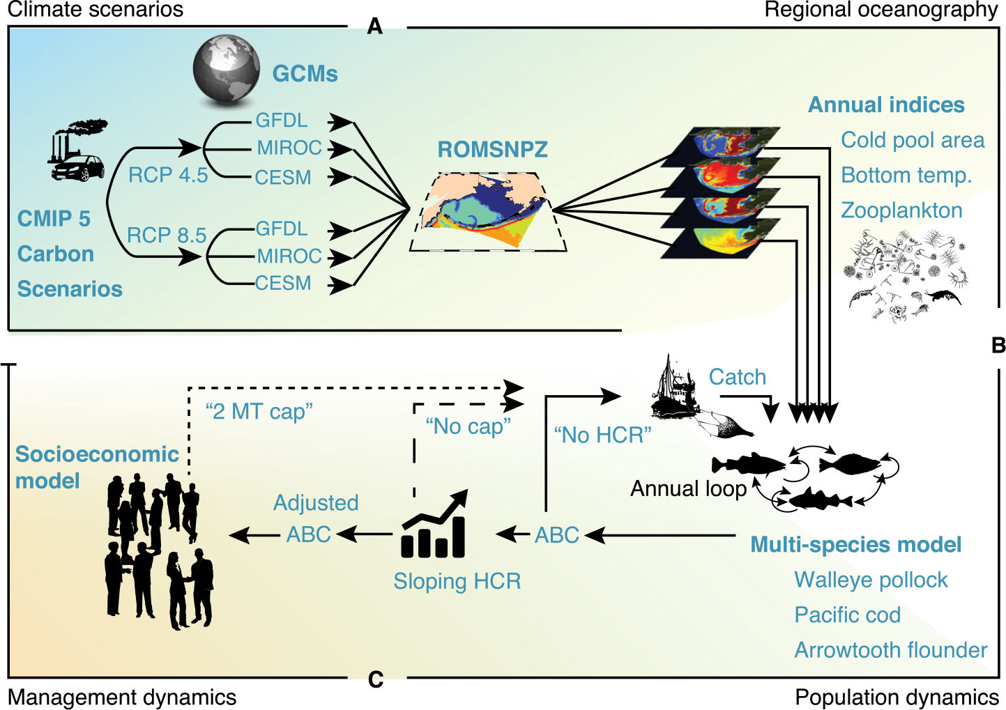
FIGURE 3. Flowchart illustrating Regional Ocean Modeling System (ROMS)-based downscaling of global climate projections to regional scale in the Bering Sea for use in Management Strategy Evaluation. From ACLIM program, Holsman et al. (2020). > High res figure

 

Integration of Modeling and Observations

Integration of modeling and observations is critical to modeling success. All ocean models have finite spatial and temporal resolution and contain multiple sources of uncertainty and imperfectly constrained parameters. Hence, validation and tuning (and/or formal data assimilation) using in situ and remotely sensed data are essential parts of the modeling process (Figure 4). Beginning with our use of SPEM, data from dedicated moorings in Shelikof Strait were used to confirm that our hydrodynamic model was capturing the essential spatial patterns of the Alaska Coastal Current. Numerous repeat transects and less common broad surveys in the GOA and the Bering Sea helped to confirm temperature, salinity, nutrients, and chlorophyll patterns were sufficiently realistic for the models to be used in process studies. Over the years, a wide array of pioneering measurements conducted by PMEL and the AFSC EcoFOCI group have been fundamental to the validation of our regional models. These data assets have included cruise-based transects of temperature and salinity, trawl surveys of bottom temperature, satellite-tracked drifters, and gliders. More recently, this family of instruments has expanded to use sensors onboard uncrewed saildrones (Stabeno et al., 2023, in this issue). The gold standard for model validation is, however, long-term time series (e.g., temperature, salinity, currents, chlorophyll fluorescence) at fixed locations throughout the water columns. These moorings are capable of capturing both short-term dynamics and long-term trends. Within EcoFOCI, the long-term moorings along the 70 m isobath in the Bering Sea (Stabeno et al., 2023, in this issue) have been fundamental to our success in modeling the Bering Sea shelf.

 

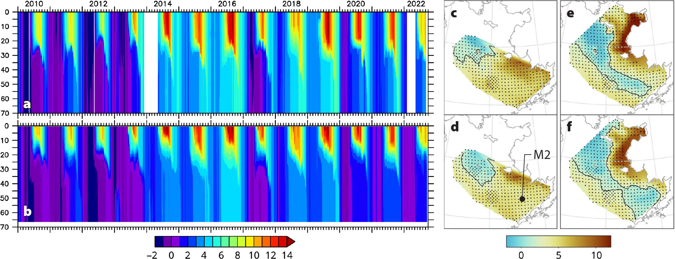
FIGURE 4. (left) Comparison of (a) biophysical mooring temperature data (°C) with (b) ROMS model output at station M2, a long-term (1995–present) biophysical mooring maintained by EcoFOCI in the southeastern Bering Sea. (right) Comparison of measured July bottom temperatures from field surveys (c,e) with modeled bottom temperatures (d,f), illustrating warm (2016; c,d) and cold (2017; e,f) years. Small black dots indicate sampling locations; large black dot indicates location of station M2 (56.87°N, 164.06°W). From Kearney et al. (2020). > High res figure

 

Serving Output to the Wider Community

Visualization of Output

Over many years, our capabilities at PMEL to visualize model output have grown more sophisticated. Initially, we displayed model results using simple contour plots—the standard currency of the oceanographic community at that time. In the 1990s, shaded plots (many generated via PMEL’s Ferret software) gradually became the new standard. In addition, at PMEL we began offering animated float tracks from the models on our web pages. As web capabilities grew, we expanded into three-dimensional displays of float tracks, which could reveal motions not easily grasped on a flat page. Several projects advanced our capabilities for low-cost immersive display of float tracks, surfaces, and volumes (immersive as in “virtual reality,” where binocular vision is a key element). Setups that ranged from displays with red-blue and polarizing glasses to active headgear were subsequently taken on the road to conferences and used for local scientific outreach at schools and science fairs. These low-cost efforts were possible due to market demands as the computer gaming community sought more lifelike experiences. Augmented reality glasses may be the next level in this evolution of scientific visualization.

 

Public Access and Partnerships

A key element of NOAA’s mission is to serve oceanic data to the public. In earlier decades, we posted animated contour plots of sea surface height, surface temperatures, and salinity from SPEM on public web pages. Ultimately, the Live Access Server (LAS), developed by the PMEL IT group, was used to host full three-dimensional output from model runs. The LAS provides interactive selection of data by region and time, as well as interactive downloading of the selected set. Most recently, the full runs of ACLIM and hindcast model output, spanning multiple decades, are being hosted on LAS and the OpenDAP service on the PMEL web server. The latter provides a means for any user to access subsets of the data from local analysis software (e.g., Ferret, MATLAB, Python, R) without needing to download the entire (terabyte-sized) set.

 

Challenges and Future Directions

Many challenges remain for successful modeling at high latitudes, especially when both physical and biological elements are contained in the same system. Continued advancements in computing and storage capacity will permit us to refine our spatial focus, enhance our trophic resolution, and expand our ensembles, yielding more statistically sound forecasts and projections despite unavoidable uncertainty.

At seasonal scales, limited capacity to predict large-scale atmospheric drivers of ocean dynamics, such as the intensity and direction of subarctic winds, hampers our ability to predict hydrodynamics of the regional ocean (e.g., temperature, currents, and sea ice) more than a few months in advance. Within fisheries, uncertainty in spawning patterns and predation, coupled with the physical uncertainty, has limited our ability to predict at the seasonal level, yet significant progress has been made (Tomassi et al., 2017). On multidecadal timescales, the largest hydrodynamic uncertainty stems from human behavior itself, that is, society’s willingness and ability to limit further emission of greenhouse gases. On top of this, future ocean ecosystems will likely be dominated by markedly different species assemblages—making any future biological patterns difficult to predict in detail. We can, however, make spatially and temporally averaged projections that are useful in management strategy evaluations. Increased computing power, dedicated field observations, and new techniques for data assimilation continue to expand our abilities to predict the regional ocean on seasonal timescales and to project a wide ensemble of possible futures.

The intermittent presence of sea ice and limited human and computer power have restricted our use of data assimilation in the past. Nonetheless, we anticipate that increasing observations at PMEL will lead to better validated, bias-corrected hindcasts, and that formal data assimilation of these assets will ultimately become common for hindcasts at PMEL.

We expect to continue strong collaboration across NOAA, which will benefit fisheries management. Although their end goals may differ, the work of physical, biological, and sociological research units focused on high latitudes are all enhanced by more accurate and refined estimates of the ocean states—past, present, and future. Sustained support, such as that provided by the NOAA Climate Ecosystems and Fisheries Initiative, will accelerate these efforts, serving as a catalyst for cross-laboratory collaboration. Under this banner, we expect these research efforts will be increasingly operationalized in order to provide regularly updated hindcasts, seasonal predictions, and long-term projections of the biophysical states of the Northeast Pacific, the Bering Sea, and the Pacific Arctic.

 

Acknowledgments

We thank a broad array of collaborators, and especially Dale Haidvogel, Enrique Curchitser, and Kate Hedstrom, for their wise counsel and contributions over many years. This publication is partially funded by the Cooperative Institute for Climate, Ocean, and Ecosystem Studies (CICOES) under NOAA Cooperative Agreement NA20OAR4320271, Contribution No. 2023-1304. This is PMEL contribution number 5491 and EcoFOCI contribution number 1036.

Hermann, A.J., W. Cheng, P.J. Stabeno, D.J. Pilcher, K.A. Kearney, and K.K. Holsman. 2023. Applications of biophysical modeling to Pacific high-​latitude ecosystems. Oceanography 36(2–3):101–108, https://doi.org/10.5670/oceanog.2023.226.

Adcroft, A., W. Anderson, V. Balaji, C. Blanton, M. Bushuk, C.O. Dufour, J.P. Dunne, S.M. Griffies, R. Hallberg, M.J. Harrison, and others. 2019. The GFDL Global Ocean and Sea Ice Model OM4.0: Model description and simulation features. Journal of Advances in Modeling Earth Systems 11(10):3,167–3,211, https://doi.org/​10.1029/2019MS001726.

Cheng, W., A. Hermann, A. Hollowed, K. Holsman, K. Kearney, D. Pilcher, C. Stock, and K. Aydin. 2021. Eastern Bering Sea shelf environmental and lower trophic level responses to climate forcing: Results of dynamical downscaling from CMIP6. Deep-Sea Research Part II 193:104975, https://doi.org/​10.1016/j.dsr2.​2021.104975.

Coyle, K.O., A.J. Hermann, and R.R. Hopcroft. 2019. Modeled spatial-temporal distribution of productivity, chlorophyll, iron and nitrate on the northern Gulf of Alaska shelf relative to field observations. Deep Sea Research Part II 165:163–191, https://doi.org/​10.1016/j.dsr2.2019.05.006.

Curchitser, E.N., H.P. Batchelder, D.B. Haidvogel, J. Fiechter, J. and Runge. 2013. Advances in physical, biological, and coupled ocean models during the US GLOBEC program. Oceanography 26(4):52–67, https://doi.org/​10.5670/oceanog.2013.75.

Danielson, S., E. Curchitser, K. Hedstrom, T. Weingartner, and P. Stabeno. 2011. On ocean and sea ice modes of variability in the Bering Sea. Journal of Geophysical Research: Oceans 116(C12), https://doi.org/10.1029/2011JC007389.

Doyle, M.J., S.L. Strom, K.O. Coyle, A.J. Hermann, C. Ladd, A. Matarese, S.K. Shotwell, and R.R. Hopcroft. 2019. Early life history phenology among Gulf of Alaska fish species: Strategies, synchronies, and sensitivities. Deep Sea Research Part II 165:41–73, https://doi.org/10.1016/j.dsr2.​2019.06.005.

Drenkard, E.J., C. Stock, A.C. Ross, K.W. Dixon, A. Adcroft, M. Alexander, V. Balaji, S.J. Bograd, M. Butenschön, W. Cheng, and others. 2021. Next-generation regional ocean projections for living marine resource management in a changing climate. ICES Journal of Marine Science 78(6):1,969–1,987, https://doi.org/10.1093/icesjms/fsab100.

Gibson, G.A., M.R. Baker, W.T. Stockhausen, S. Hinckley, C. Parada, K.O. Coyle, K. Aydin, A.J. Hermann, T. Hurst, and A.E. Punt. 2022. Modeling in an Integrated Ecosystem Research framework to explore recruitment in Gulf of Alaska groundfish – Applications to management and lessons learned. Deep-Sea Research Part II 197:105048, https://doi.org/10.1016/​j.dsr2.2022.105048.

Haidvogel, D.B., J.L. Wilkin, and R. Young. 1991. A semi-spectral primitive equation ocean circulation model using vertical sigma and orthogonal curvilinear horizontal coordinates. Journal of Computational Physics 94:151–185, https://doi.org/​10.1016/​0021-9991(91)90141-7.

Haidvogel, D.B., H. Arango, W.P. Budgell, B.D. Cornuelle, E. Curchitser, E. Di Lorenzo, K. Fennel, W.R. Geyer, A.J. Hermann, L. Lanerolle, and others. 2008. Ocean forecasting in terrain-​following coordinates: Model formulation and skill assessment of the Regional Ocean Modeling System. Journal of Computational Physics 227:3,595–3,624, https://doi.org/10.1016/​j.jcp.2007.06.016.

Hermann, A.J., and P.J. Stabeno. 1996. An eddy resolving model of circulation on the western Gulf of Alaska shelf: Part I. Model development and sensitivity analyses. Journal of Geophysical Research: Oceans 101:1,129–1,149, https://doi.org/​10.1029/95JC02681.

Hermann, A.J., G.A. Gibson, W. Cheng, I. Ortiz, K. Aydin, M. Wang, A.B. Hollowed, and K.K. Holsman. 2019. Projected biophysical conditions of the Bering Sea to 2100 under multiple emission scenarios. ICES Journal of Marine Science 76(5):1,280–1,304, https://doi.org/10.1093/icesjms/fsz043.

Hermann, A.J., K. Kearney, W. Cheng, D. Pilcher, K. Aydin, K.K. Holsman, and A.B. Hollowed. 2021. Coupled modes of projected regional change in the Bering Sea from a dynamically downscaling model under CMIP6 forcing. Deep Sea Research Part II 194:104974, https://doi.org/10.1016/j.dsr2.​2021.104974.

Hinckley, S., J.M. Napp, A.J. Hermann, and C. Parada. 2009. Simulation of physically mediated variability in prey resources of a larval fish: a three-dimensional NPZ model. Fisheries Oceanography 18(4):201–223, https://doi.org/​10.1111/j.1365-2419.2009.00505.x.

Hollowed, A.B., K.K. Holsman, A.C. Haynie, A.J. Hermann, A.E. Punt, K. Aydin, J.N. Ianelli, S. Kasperski, W. Cheng, A. Faig, and others. 2020. Integrated modeling to evaluate climate change impacts on coupled social-ecological systems in Alaska. Frontiers in Marine Science 6:775, https://doi.org/10.3389/fmars.2019.00775.

Holsman, K.K. A.C. Haynie, A.B. Hollowed, J.C.P. Reum, K. Aydin, A.J. Hermann, W. Cheng, A. Faig, J.N. Ianelli, K.A. Kearney, and A.E. Punt. 2020. Ecosystem-based fisheries management forestalls climate-driven collapse. Nature Communications 11:4579, https://doi.org/10.1038/s41467-020-18300-3.

Hunt, G.L. Jr, K.O. Coyle, L.B. Eisner, E.V. Farley, R.A. Heintz, F. Mueter, J.M. Napp, J.E. Overland, P.H. Ressler, S. Salo, and P.J. Stabeno. 2011. Climate impacts on eastern Bering Sea foodwebs: A synthesis of new data and an assessment of the Oscillating Control Hypothesis. ICES Journal of Marine Science 68(6):1,230–1,243, https://doi.org/​10.1093/icesjms/fsr036.

Kearney, K. 2020. ROMS Modeled bottom temperature. Pp 69–71 in Ecosystem Status Report 2020: Eastern Bering Sea, Stock Assessment and Fishery Evaluation Report. E. Siddon, ed., North Pacific Fishery Management Council, Anchorage, Alaska.

Kearney, K., A. Hermann, W. Cheng, I. Ortiz, and K. Aydin. 2020. A coupled pelagic-benthic-​sympagic biogeochemical model for the Bering Sea: Documentation and validation of the BESTNPZ model (v2019.08.23) within a high-​resolution regional ocean model. Geoscientific Model Development 13:597–650, https://doi.org/​10.5194/gmd-13-597-2020.

Kearney, K.A., M. Alexander, K. Aydin, W. Cheng, A. Hermann, G. Hervieux, and I. Ortiz. 2021. Seasonal predictability of sea ice and bottom temperature across the eastern Bering Sea shelf. Journal of Geophysical Research: Oceans 126:e2021JC017545, https://doi.org/​10.1029/2021JC017545.

Mordy, C.W., N.A. Bond, E.D. Cokelet, A. Deary, E. Lemagie, P. Proctor, P.J. Stabeno, H.M. Tabisola, T. Van Pelt, and E. Wisegarver. 2023. Progress of fisheries-​oceanography coordinated investigations in the Gulf of Alaska and Aleutian Passes. Oceanography 36(2–3):94–100, https://doi.org/​10.5670/oceanog.2023.218.

Ortiz, I., K. Aydin, A. Hermann, G. Gibson, A. Punt, F.K. Wiese, L.B. Eisner, N. Ferm, T.W. Buckley, E.A. Moffit, J.N. Ianelli, and others. 2016. Climate to fish: Synthesizing field work, data and models in a 39-year retrospective analysis of seasonal processes on the eastern Bering Sea shelf and slope. Deep Sea Research Part II 134:390–412, https://doi.org/​10.1016/j.dsr2.2016.07.009.

Pilcher, D.J., D.M. Naiman, J.N. Cross, A.J. Hermann, S.A. Siedlecki, G.A. Gibson, and J.T. Mathis. 2019. Modeled effect of coastal biogeochemical processes, climate variability, and ocean acidification on aragonite saturation state in the Bering Sea. Frontiers in Marine Science 5:508, https://doi.org/​10.3389/fmars.2018.00508.

Pilcher, D.J., J.N. Cross, A. Hermann, K. Kearney, W. Cheng, and J.T. Mathis. 2022. Dynamically downscaled projections of ocean acidification for the Bering Sea, Deep Sea Research Part II 198:105055, https://doi.org/10.1016/j.dsr2.​2022.105055.

Siedlecki, S.A., S.R. Alin, E.L. Norton, N.A. Bond, A.J. Hermann, R.A. Feely, and J.A. Newton. 2023. Can seasonal forecasts of ocean conditions aid fishery managers? Experiences from 10 years of J-SCOPE. Oceanography 36(2–3):158–167, https://doi.org/​10.5670/oceanog.2023.219.

Song, Y., and D.B. Haidvogel. 1994. A semi-​implicit ocean circulation model using a generalized topography-​following coordinate system. Journal of Computational Research 115:228–244, https://doi.org/10.1006/jcph.1994.1189.

Stabeno. P.J., and A.J. Hermann. 1996. An eddy resolving model of circulation on the western Gulf of Alaska shelf: Part II. Comparison of results to oceanic observations. Journal of Geophysical Research: Oceans 101:1,151–1,161, https://doi.org/​10.1029/95JC02682.

Stabeno, P.J., S. Bell, C. Berchok, E.D. Cokelet, J. Cross, R.M. McCabe, C.W. Mordy, J. Overland, D. Strausz, M. Sullivan, and H.M. Tabisola. 2023. Long-term biophysical observations and climate impacts in US Arctic marine ecosystems. Oceanography 36(2–3):78–85, https://doi.org/​10.5670/oceanog.2023.225.

Tommasi, D., C.A. Stock, A.J. Hobday, R. Methot, I.C. Kaplan, J.P. Eveson, K. Holsman, T.J. Miller, S. Gaichas, M. Gehlen, and others. 2017. Managing living marine resources in a dynamic environment: The role of seasonal to decadal climate forecasts. Progress in Oceanography 152:15–49, https://doi.org/​10.1016/j.pocean.2016.12.011.

This is an open access article made available under the terms of the Creative Commons Attribution 4.0 International License (https://creativecommons.org/licenses/by/4.0/), which permits use, sharing, adaptation, distribution, and reproduction in any medium or format as long as users cite the materials appropriately, provide a link to the Creative Commons license, and indicate the changes that were made to the original content. Images, animations, videos, or other third-party material used in articles are included in the Creative Commons license unless indicated otherwise in a credit line to the material. If the material is not included in the article’s Creative Commons license, users will need to obtain permission directly from the license holder to reproduce the material.