We provide a high-level review of sea ice models used for climate studies and of the recent advances made with these models to understand sea ice predictability. Models currently in use for the Coupled Model Intercomparison Project and new developments coming online that will enable enhanced predictions are discussed. Previous work indicates that seasonal sea ice can be predicted based on mechanisms associated with long-lived ice thickness or ocean heat anomalies. On longer timescales, internal climate variability is an important source of uncertainty, although anthropogenic forcing is sizable, and studies suggest that anthropogenic signals have already emerged from internal climate noise. Using new analysis from the Multi-Model Large Ensemble, we show that while models differ in the magnitude and timing of predictable signals, many ice predictability characteristics are robust across multiple models. This includes the reemergence of predictable seasonal signals in ice area and the sizable uncertainty in predictions of ice-free Arctic timing associated with internal variability.

Photo courtesy of Melinda Webster, University of Alaska Fairbanks. > High res figure

Introduction

On average, 25 million square kilometers of sea ice float on the world’s high-​latitude oceans. Sea ice is frozen ocean—a complicated, dynamic, semisolid mixture of ice, water, salt, and gases. Although sea ice is found primarily in the polar regions, it strongly influences the weather and climate of the entire Earth and has a profound impact on the industries, wildlife, and people who contend with it year-round.

Sea ice forms as seawater freezes, becoming a floating barrier between the air and ocean that reflects solar radiation and impedes transfers of heat and mass. The Arctic climate is changing quickly with September Arctic ice extent declining by over 13% per decade since 1979 (e.g., Serreze and Stroeve, 2015). Climate models predict that September Arctic ice-free conditions are likely by mid-century (e.g., Jahn, 2018). The ice volume is critical for the resiliency of the ice pack under changing environmental conditions; predictions of future sea ice change depend in part on the simulated late twentieth century ice thickness (Massonnet et al., 2018). Ice thickness determines the sensitivity of the ice to melting and freezing, and the area covered by ice increases planetary albedo, the reflection of radiation back to space.

Because of large-scale ice loss, there is growing interest in safe Arctic marine access and a need for reliable predictions on seasonal to interannual time­scales. Predictions on multi-decadal scales are also needed for infrastructure planning and to inform climate mitigation and adaptation measures. Earth system model studies have provided new insights on sea ice predictability across timescales. A better understanding of predictability, or the characteristics that enable prediction, provides useful information for building more skillful forecast systems.

Predictability arises from two distinct factors. On shorter timescales, the initial state of the system and dynamics that retain some “memory” of that initial state are sources of predictability. For atmospheric weather forecasts, this “initial-value predictability” enables skillful operational forecasts for about a week (e.g., Krishnamurthy, 2019). For slower evolving components of the system, including the ocean and sea ice, it can enable forecasts on seasonal to interannual timescales (e.g., Blanchard-Wrigglesworth et al., 2011a). Another source of predictability resides in climate drivers, such as rising greenhouse gas concentrations, which elicit a predictable response in the Earth system (e.g., Manabe and Stouffer, 1980). This “boundary forced predictability” enables projections of Arctic sea ice loss on decadal timescales (e.g., Blanchard-Wrigglesworth et al., 2011b) and the predictable transition to ice-free Arctic summers (e.g., Jahn et al., 2016) in response to future scenarios of rising greenhouse gases.

Modeling coupled interactions of sea ice with the atmosphere, the ocean, and nearshore topography are critical for reliable predictions across timescales. Predictions of sea ice properties, such as landfast ice and wave-ice interactions, have required new ice model developments. During the last decade, such developments have led to improved representation of coupled interactions and enhanced realism of the simulated sea ice itself.

In the next section we discuss sea ice models used for climate applications and then advances that have been made with those models for understanding and predicting Arctic sea ice variability and change. In the last section, we outline new developments that are coming online and their implications for sea ice predictive capabilities.

 

Sea Ice Models Used for Climate Applications

Sea ice is a mixture of open water, thin first-year ice, thicker multiyear ice, and thick pressure ridges. A complex combination of thermal, radiative, kinematic, and mechanical processes determines the composition, structure, and volume of sea ice. Climate simulations require a conservative, consistent, physically accurate representation of sea ice’s interactions with the ocean and atmosphere. For models in the recent Coupled Model Intercomparison Project (CMIP; Eyring et al., 2016), the sea ice component consists of a momentum and rheology model for ice motion, a transport model that conserves ice volume and other quantities as the ice deforms and moves, and vertical physics including mechanical and thermodynamic models to compute ice thickness evolution. Keen et al. (2021) summarize the sea ice options used within CMIP6. Newer sea ice models incorporate biology, chemistry, landfast ice, wave-ice interactions, and advanced snow properties, although these developments are not yet routinely used in climate simulations.

Arguably, the most critical sea ice role in the climate system is thermodynamic: snow-covered ice is among the most reflective natural materials, and ice and its overlying snow cover effectively insulate the atmosphere from the ocean. Heat conduction through the ice and snow affects the surface heat flux and determines phase changes throughout the ice (e.g., Maykut and Untersteiner, 1971). Heat tends to flow upward, from the warm ocean toward the colder atmosphere, so sea ice thermodynamics can be represented within a vertical column. Total freezing or melting is computed based on ice-ocean and ice-atmosphere heat exchange, vertically resolved temperatures, and resulting vertical heat conduction.

Representing hydrologic properties, such as liquid water on top of and within the ice, is critical for accurately simulating ice pack evolution. Most CMIP6 sea ice model components employ a basic heat conduction model for the snow, incorporating melt and associated albedo changes along with more complex processes such as snow-ice formation due to flooding and snow infiltration by meltwater, which may form melt ponds. New snow model developments such as wind-driven compaction and drifting of snow into the ocean are now being adopted in climate models (e.g., Lecomte et al., 2013).

For climate-scale simulations, which have spatial resolutions of tens to hundreds of kilometers, many processes require sub-gridscale resolution for improved fidelity. This is captured via an ice thickness distribution (ITD), which computes the horizontal area covered by a given range of ice thickness within a grid cell (e.g., Thorndike et al., 1975). Thermodynamic quantities, including ice growth/melt rates and surface fluxes, are computed for each thickness category. Dynamic properties are also a function of the ITD; for example, ice strength can be modeled as a simple function of ice thickness and concentration (Hibler, 1979), or through an energy-based description tied to the ITD (Thorndike et al., 1975). Inclusion of an ITD influences coupled climate feedbacks (Holland et al., 2006) with implications for climate prediction.

Sea ice surface albedo is computed based on the surface fractions of snow, melt ponds, and bare ice. Because reflectivity differs considerably for these surfaces (Perovich et al., 2002), the relative fractional surface types and how they vary over time affects the surface albedo feedback (Holland and Landrum, 2015). Ice-atmosphere fluxes change the surface characteristics (e.g., melting snow pools into ponds), which then alter the albedo and fluxes. Hydrologic changes also occur. While some models use an empirical relationship between sea ice albedo and ice thickness and surface temperatures, other models apply inherent optical properties to calculate the complex scattering of light within the ice and snow, and the resulting albedos (Briegleb and Light, 2007). Absorbed radiation also induces hydrologic changes, and “mushy” thermodynamic approaches treating sea ice as a two-phase material of brine and ice have been introduced into models (e.g., Vancoppenolle et al., 2009; Turner and Hunke, 2015).

The simplest parameterization of melt ponds empirically adjusts the surface albedo based on the modeled surface temperature and snow depth. More complex, explicit parameterizations (Flocco et al., 2012; Hunke et al., 2013) carry volume and area of meltwater pools on the ice, sourced from ice melt, snow melt, and rainfall. Snow may shield a pond from solar radiation, resulting in radiatively “effective” pond properties used for the shortwave radiation calculation.

Ice velocity is determined by wind, ocean currents, sea surface slope, Coriolis force, contact with land surfaces, and a constitutive model that represents ice strength and rheology. Cracks and ridges in the ice form due to velocity-derived deformation, allowing the direct flux of moisture and heat between the ocean and the atmosphere. Many CMIP6 models use the elastic-viscous-plastic (EVP) rheology (Hunke and Dukowicz, 1997), which introduced an elastic term into the viscous-plastic (VP; Hibler, 1979) ice constitutive equation for computational efficiency. Efficient, monotone, and accurate schemes advect multiple tracers with the ice (Lipscomb and Hunke, 2004).

Neither the model capabilities outlined in this section nor their references are exhaustive here. Newer model developments likely to be incorporated in future climate modeling studies (see later section on Sea Ice Model Advances) are partly driven by the need to better understand the predictability properties of sea ice in climate-scale simulations.

 

Using Models to Predict Arctic Sea Ice

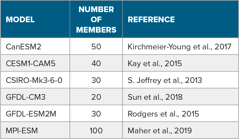
Sea ice components have been coupled within Earth system models to enable climate studies. These models freely evolve based on internal dynamics and coupled interactions and prescribe climate drivers such as changes in greenhouse gas concentrations (GHGs) or volcanic emissions. Coordinated experiments (e.g., Eyring et al., 2016), and large ensembles from individual models (e.g., Deser et al., 2020) have resulted in a deeper understanding of sea ice predictability and change. Although structural model uncertainty remains important, many findings are robust across models. In this section we discuss how Earth system models have enhanced our understanding of sea ice and its predictability. We explore some of these factors using results from the multi-model large ensemble (MMLE; Deser et al., 2020; Table 1).

 

TABLE 1. The models used in the multi-model large ensemble (MMLE). > High res table

 

Historical Sea Ice Loss

Climate variations result from external climate drivers (“forced change”) arising from both natural and anthropogenic factors, and from internal dynamics (“internal variability”) associated with the chaotic system. Simulations that prescribe specific time-varying climate drivers, for example, only GHGs or only natural drivers such as volcanic emissions, indicate that anthropogenic GHGs have played a significant role in historical Arctic ice loss (e.g., Min et al., 2008), with cooling from anthropogenic aerosols offsetting the ice decline by about 23% (Mueller et al., 2018).

In large ensembles of simulations with individual CMIP-class models, differences between ensemble members reflect simulated internal variability. These ensembles have clarified the sizable role of internal variability in many climate properties. For Arctic sea ice, internal variability has a large influence on multi-decadal trends (e.g., Swart et al., 2015), a consistent result across models. Studies suggest that internal variability has reinforced anthropogenic September Arctic ice loss since 1979. For example, by assuming that the mean change from a single model ensemble is a realistic forced response, Kay et al. (2011) found that internal variability accounted for ~50% of the observed 1979–2005 September ice loss.

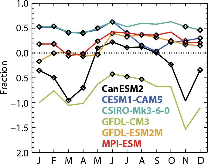
A robust quantification of the role of internal variability in observed trends is difficult given potential model biases. Comparing large ensembles from multiple models illustrates this challenge. In Figure 1, the fraction of observed ice loss associated with internal variability in the MMLE assumes that an individual model’s ensemble mean realistically simulates the externally forced trend. Five of six models suggest that summer ice loss has been enhanced by internal variability, although the magnitude varies. For the remainder of the year, most models also suggest that internal variability has reinforced sea ice loss, although two models (CanESM2 and GFDL-CM3) consistently suggest that internal variability has counteracted forced loss for these months. Notably, for GFDL-CM3 in all months except June–August and CSIRO-Mk3-6-0 for July–October, the ensemble distribution of ice loss is not consistent with observations.

 

FIGURE 1. The fraction of 1979–2018 observed ice area loss attributed to internal variability from multi-model large ensemble (MMLE) results. Diamonds indicate months when the envelope of the model ensemble spread in 1979–2018 trends encompass the observed trend. Assuming enough members to characterize internal variability, this is a minimum requirement that simulated trends are consistent with observations. > High res figure

 

These attribution disparities are related to differences in mean ice area and thickness, which could allow for some observational constraints on the attribution. Alternatively, assessing simulated mechanisms of internal variability and comparing these to observations provides a mechanistic approach. For example, Ding et al. (2019) diagnosed “fingerprints” of internal historical ice loss variability and found enhanced loss in simulations with increasing Arctic atmospheric pressure. The atmospheric circulation variability strongly corresponds with observed changes, estimated to contribute 40%–50% of the observed 1979–2015 summer ice loss. A similar relationship between Beaufort Sea atmospheric pressure and Arctic ice cover emerged from a perturbed-​parameter climate model ensemble (Urrego-Blanco et al., 2019). Roach and Blanchard-Wrigglesworth (2022), using experiments in which winds were nudged to observations, also found that observed wind variations reinforced summer ice loss, but played little role in historical winter/spring sea ice trends.

 

Initial-Value Sea Ice Prediction

Because of sea ice loss, there is growing interest in safe Arctic marine access, and this has spurred interest in predicting sea ice across timescales from seasonal to multi-decadal (e.g., Eicken, 2013; Melia et al., 2017). Earth system models have provided insights on sea ice predictability associated with initial conditions (“initial-value predictability”), including analysis of diagnostic predictability from the correlation structure of simulated conditions, inherent predictability from “perfect model” studies that assess the ability of the model to predict itself, and studies with forecasting systems initialized with observed conditions. There is strong evidence of the potential for skillful seasonal ice predictions and consistency on the fundamental sources of that predictability. These insights are informing the development of improved prediction systems.

Blanchard-Wrigglesworth et al. (2011a) assessed the autocorrelation of Arctic ice extent from a large ensemble and provided a metric for diagnostic predictability. They found that ice anomalies exhibit a persistence of several months and a “reemergence” of memory for some times of year. This includes (1) a summer-​to-​summer reemergence associated with long-​lived ice thickness anomalies, and (2) a melt-​to-​freeze season reemergence associated with long-lived ocean heat content anomalies. These sources of memory have been confirmed in additional studies (e.g., see Guemas et al., 2016, for a review). They should enable predictive skill on these timescales, while pointing to aspects of the system that need to be well-initialized to realize that skill.

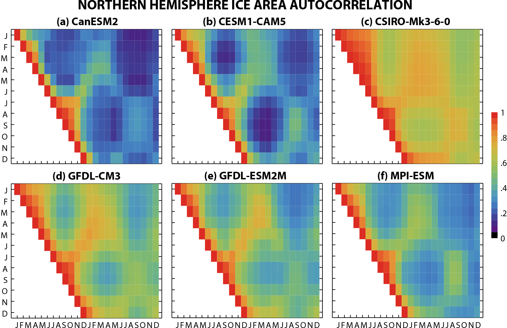
In the MMLE (Figure 2), we find that all models exhibit these predictability features, with a two- to three-month “persistence timescale” over which the autocorrelation declines. For ice area in February through May (y-axis), relatively low correlations after two to three months are followed by an increase in correlation during the ice growth season (approximately January–March, x-axis), indicating the melt-to-freeze season reemergence. Correlations for summer months (August–October) exhibit a summer-to-summer reemergence with enhanced correlations at a one-year lag. While the consistency across the models in these and other properties has been highlighted in several studies, the models differ in the magnitude and timing of predictable signals, which are related in part to different climate state properties (e.g., Day et al., 2014b), providing optimization opportunities for sea ice prediction.

 

FIGURE 2. Autocorrelation of Northern Hemisphere ice area anomalies from MMLE models using data from 1960–2000 and all ensemble members. Ice anomalies on the y-axis month are correlated with future anomalies shown on the x-axis. To isolate anomalies from internal variability, the ensemble mean is removed from each model. > High res figure

 

Comparisons across models indicate that climate properties can affect ice predictability—not surprising since the mean ice state influences sea ice feedbacks (e.g., Massonnet et al. 2018)—and suggest that initial-value predictability might change in a warming climate. Indeed, Holland et al. (2019) found that summer ice predictability changes as the climate warms, because the growth of ice thickness initialization errors and their role in summer melt-out depend on the mean sea ice state. These factors can help explain across-model differences in predictability.

Idealized studies indicate that skillful seasonal predictions of ice area should be possible for both pan-Arctic and regional domains. Forecasting systems initialized with observations have been developed to realize this predictability (e.g., Hunke et al., 2020) and exhibit skill in retrospective, seasonal predictions (e.g., Guemas et al. 2016). These systems are also being used to inform data assimilation needs. For example, Bushuk et al. (2019) assessed the importance of different initial conditions for Barents Sea ice predictions by removing certain assimilated observations. They found that sea surface temperatures were important for predictions on interannual timescales, and deeper ocean temperatures played an important role in predicted trends. Additional work has elucidated the benefit of assimilating ice thickness information for Arctic summer ice extent and ice-edge location predictions (e.g., Day et al., 2014a; Blockley and Peterson, 2018).

 

Boundary Forced Predictability and Projections of Sea Ice

On longer timescales, sea ice predictability arises from changes in climate drivers (“boundary forced predictability”). In the next decades, Arctic sea ice is projected to decline due to rising GHGs (e.g., Notz et al., 2020). However, internal variability remains an important source of uncertainty in the rate of future ice loss. Using numerous models, Bonan et al. (2021) found that internal variability accounts for 40%–60% of the summer ice loss uncertainty in the next decade, model structure uncertainty dominates in mid-​century, and future emissions uncertainty dominates at the end of the twenty-​first century. For winter sea ice, uncertainty associated with internal variability plays a role for longer lead times.

The continued influence of internal variability could mask the emergence of anthropogenically forced signals in the changing Arctic climate. A number of studies have used Earth system models to quantify when a forced signal emerges from the sizable internally generated Arctic climate variability. Even with this large noise, studies indicate that multiple aspects of forced Arctic change have emerged or will do so soon, including fall-winter surface warming (Hawkins and Sutton, 2012), an Arctic amplified signal of warming (e.g., England et al., 2021), and sea ice extent changes in both summer and winter (Landrum and Holland, 2020).

Internal variability also impacts the predictability of the timing of climate signals. For example, Jahn et al (2016) found an approximately 20-year range in the first occurrence of September ice-free Arctic conditions. An analysis of MMLE models confirms this important role of internal variability. In the ensemble mean, these models differ considerably in the timing of September ice-free conditions (Figure 3a), related in part to differences in their early twenty-​first century state: the mean timing of ice-free conditions across the models is correlated to the annual cycle amplitude of 2000–2009 Arctic mean ice thickness at R = 0.95. Regardless of the mean timing of ice-free conditions, however, the uncertainty across all the models is sizable (Figure 3b).

 

FIGURE 3. (a) Time series of ensemble-mean, Northern Hemisphere, September ice area from MMLE models. (b) Timing of first ice-free conditions, where the thin lines show the full ensemble range, the thick bars indicate the standard deviation, and the ensemble mean is indicated by white asterisks. CSIRO-Mk3-6-0 does not reach ice-free conditions by 2100. Updated from Vavrus and Holland (2021). > High res figure

 

Sea Ice Model Advances Since CMIP6 and Implications for Improved Prediction

Many advances are underway to improve the simulation of sea ice within Earth system models. While this discussion focuses on sea ice model developments, their most significant climate impacts will be through their influence on feedbacks between the ice, atmosphere, and ocean. Better simulation of climate feedbacks will influence sea ice prediction. New ice model capabilities also allow for predictions of additional sea ice features (e.g., landfast ice) relevant to stakeholders. Although not a comprehensive list, here we describe some developments under consideration for the next class of coupled earth system models.

While plastic deformation produced by the (E)VP model approximates ice deformation (e.g., Mehlmann et al., 2021), recent improvements include Elastic Anisotropic Plastic (EAP) dynamics (Wilchinsky and Feltham, 2006; Tsamados et al., 2013), which accounts for subgrid regions of weakness in the ice cover that allow the ice to fracture in preferred directions. Brittle rheologies that incorporate damage are also being implemented in large-scale models.

Landfast ice—ice fastened to the coastline or seabed and lacking motion—is used by coastal communities for travel and hunting. As a solid barrier between the ocean and atmosphere, it limits direct fluxes of moisture and heat and can block a river’s flow and cause flooding. A stress term added to the momentum equation better characterizes the interactions between grounded ridges and the seabed, improving the simulation of landfast ice in shallow water (Lemieux et al., 2016). To better simulate landfast ice in deeper water, the tensile strength of fixed, consolidated ice was also modified.

Areas covered by floes of different horizontal sizes have been represented using a floe size distribution analogous to the ice thickness distribution (Roach et al., 2018). Floe sizes change through five processes: new ice formation, welding of floes in freezing conditions, lateral growth, melt, and fracture of floes by surface waves. Fragmentation by waves makes ice more susceptible to summer melt and determines whether ice forms as pancakes or larger floes during freeze-up; this also influences ocean-atmosphere interactions. In the future, ice floe size characteristics will be used to influence waves in ocean models. Floe size can also influence drag by wind and currents on the ice surface. Most climate models use constant drag coefficients, but new developments allow the drag coefficients to depend on the ridges and keels of deformed ice and on ice edges (Tsamados et al., 2014).

New developments in modeling also focus on biogeochemistry and ecosystem dynamics (e.g., Duarte et al., 2017; N. Jeffrey et al., 2020) by tightly coupling ice physics and the chemistry and biology within the brine network. When ice forms, the crystalline structure extrudes brine, some of which is captured in pockets within the ice. These brine pockets expand and contract with changing temperature, becoming conduits for meltwater and nutrient-​laden seawater. Organisms such as algae that live within the brine network, seed oceanic algal blooms in winter and early spring, thus serving as a fundamental source for primary production in polar waters. Incorporation of sea ice biogeochemistry into Earth system models will enable better prediction of marine ecosystems. It will also influence coupled feedbacks as ice algal production affects the flux of dimethyl sulfide (DMS), which is important in forming cloud
condensation nuclei.

While sea ice predictions hinge crucially on interactions with the atmosphere and ocean, some developments target internal sea ice model representations for improved short-term or fine spatial scale predictions. These new approaches have the potential to revolutionize the representation of sea ice in climate simulations. For instance, the neXtSIM model (Rampal et al., 2016) uses a Lagrangian advection scheme in which the mesh moves with the ice, employing a brittle rheology to simulate properties of ice drift and deformation. New efforts to capture both Lagrangian and anisotropic sea ice behavior include discrete element modeling (Herman, 2016) in which aggregates of ice floes form the numerical elements.

Such advances will enable more realistic interactions with the atmosphere and ocean models and provide the capability to simulate more complex sea ice features. This will ultimately allow for enhanced prediction of stakeholder-relevant aspects of the changing Arctic. Note however that predictions of sea ice are also strongly influenced by the simulated atmosphere and ocean, and so improvements in ice model processes alone are not a panacea. Thus, developments are also needed within atmospheric and oceanic models to better simulate winds, radiation fields, and ocean heat transport, among other properties.

 

Conclusions

Here we have provided a high-level review of sea ice models used for climate simulations and recent advances made with these models to understand seasonal to multi-decadal sea ice predictability. This has been enhanced with new analysis from the MMLE (Deser et al., 2020), which indicates that while many findings are robust across models, there remain model structural uncertainty that affects the magnitude of predictive signals and attribution of the factors responsible for historical ice loss. Comparison across models of simulated sea ice predictability/​variability mechanisms and their similarity to observations is needed to further elucidate factors of ice predictability and change.

Because sea ice plays a critical role in the climate system through its influence on the surface heat budget and the hydrological cycle, models need to adequately represent processes that affect these climate interactions. The sea ice components used in current Earth system models have advanced considerably in the last decade, allowing for more realistic treatment of ice dynamics, thermodynamics, and spatial heterogeneity and thus improving the simulation of climate feedbacks. New advances are continuing to improve the realism of sea ice and its interactions with the atmosphere and ocean. For example, models that simulate a floe size distribution allow for wave-ice coupling, and the incorporation of sea ice biogeochemistry enables new feedbacks for the marine ecosystem and polar cloud properties. While these elements have not yet been included in CMIP studies, they provide new avenues for research and Earth system prediction.

These advances will build on a body of research that uses Earth system models to query the predictability of Arctic sea ice. This work has shown that sea ice area is predictable on seasonal time­scales and has highlighted predictability mechanisms, thus informing ice forecasting systems for more skillful predictions. Recent research has also elucidated the critical role of internal variability in the climate system and the influence this internal variability has on multi-decadal ice trends. Evidence suggests that internal variability has reinforced anthropogenically driven summer ice loss in the Arctic by as much as 50%, with atmospheric circulation variability playing a key role. While internal variability is a sizable source of uncertainty in longer timescale predictions, anthropogenically driven changes in the Arctic are also large, and many anthropogenic Arctic climate changes have already emerged from the internal climate noise.

 

Acknowledgments

E. Hunke thanks the Earth and Environmental Systems Modeling programs of the US Department of Energy Office of Science Biological and Environmental Research. M. Holland acknowledges support from the National Center for Atmospheric Research (NCAR), a major facility sponsored by the National Science Foundation under Cooperative Agreement No. 1852977. We thank the reviewers for helpful comments that led to improvements in the manuscript. Title page background photo courtesy of Melinda Webster, University of Alaska Fairbanks.

Holland, M.M., and E.C. Hunke. 2022. A review of Arctic sea ice climate predictability in large-scale Earth system models. Oceanography 35(3–4):20–27, https://doi.org/10.5670/oceanog.2022.113.

Blanchard-Wrigglesworth, E., K.C. Armour, C.M. Bitz, and E. DeWeaver. 2011a. Persistence and inherent predictability of Arctic sea ice in a GCM ensemble and observations. Journal of Climate 24:231–250, https://doi.org/10.1175/2010JCLI3775.1.

Blanchard-Wrigglesworth, E., C.M. Bitz, and M.M. Holland. 2011b. Influence of initial conditions and climate forcing on predicting Arctic sea ice. Geophysical Research Letters 38(18), https://doi.org/​10.1029/​2011GL048807.

Blockley, E.W., and K.A. Peterson. 2018. Improving Met Office seasonal predictions of Arctic sea ice using assimilation of CryoSat-2 thickness. The Cryosphere 12(11):3,419–3438, https://doi.org/​10.5194/tc-12-3419-2018.

Bonan, D., F. Lehner, and M.M. Holland. 2021. Partitioning uncertainty in projections of Arctic sea ice. Environmental Research Letters 16:044002, https://doi.org/10.1088/1748-9326/abe0ec.

Briegleb, B.P., and B. Light. 2007. A Delta-Eddington Multiple Scattering Parameterization for Solar Radiation in the Sea Ice Component of the Community Climate System Model. NCAR Technical Note NCAR/TN-472+STR, National Center for Atmospheric Research, 108 pp.

Bushuk, M., X. Yang, M. Winton, R. Msadek, M. Harrison, A. Rosati, and R. Gudgel. 2019. The value of sustained ocean observations for sea ice predictions in the Barents Sea. Journal of Climate 32(20):7,017–7,035, https://doi.org/10.1175/JCLI-D-19-0179.1.

Day, J.J., E. Hawkins, and S. Tietsche. 2014a. Will Arctic sea ice thickness initialization improve seasonal forecast skill? Geophysical Research Letters 41(21):7,566–7,575, https://doi.org/​10.1002/2014GL061694.

Day, J.J., S. Tietsche, and E. Hawkins. 2014b. Pan-Arctic and regional sea ice predictability: Initialization month dependence. Journal of Climate 12:4,371–4,390, https://doi.org/10.1175/JCLI-D-13-00614.1.

Deser, C., F. Lehner, K.B. Rodgers, T. Ault, T.L. Delworth, P.N. DiNezio, A. Flore, C. Frankignoul, J.C. Fyfe, D.E. Horton, and others. 2020. Insights from Earth system model initial-condition large ensembles and future prospects. Nature Climate Change 10:277–286, https://doi.org/10.1038/s41558-020-0731-2.

Ding, Q., A. Schweiger, M. L’Heureux, E.J. Steig, D.S. Battisti, N.C. Johnson, E. Blanchard-Wrigglesworth, S. Po-Chedley, Q. Zhang, K. Harnos, and others. 2019. Fingerprints of internal drivers of Arctic sea ice loss in observations and model simulations. Nature Geoscience 12:28–33, https://doi.org/​10.1038/s41561-018-0256-8.

Duarte, P., A. Meyer, L.M. Olsen, H.M. Kauko, P. Assmy, A. Rösel, P. Itkin, S.R. Hudson, M.A. Granskog, S. Gerland, and others. 2017. Sea ice thermohaline ​dynamics and biogeochemistry in the Arctic Ocean: Empirical and model results. Journal of Geophysical Research: Biogeosciences 122:1,632–1,654, https://doi.org/​10.1002/2016JG003660.

Eicken, H. 2013. Arctic sea ice needs better forecasts. Nature 497(7450):431–433, https://doi.org/​10.1038/497431a.

England, M.R., I. Eisenman, N.J. Lutsko, and T.J.W. Wagner. 2021. The recent emergence of Arctic amplification. Geophysical Research Letters 48(15): e2021GL094086, https://doi.org/​10.1029/​2021GL094086.

Eyring, V., S. Bony, G.A. Meehl, C.A. Senior, B. Stevens, R.J. Stouffer, and K.E. Taylor. 2016. Overview of the Coupled Model Intercomparison Project Phase 6 (CMIP6) experimental design and organization. Geoscientific Model Development 9:1,937–1,958, https://doi.org/​10.5194/gmd-9-1937-2016.

Flocco, D., D. Schroeder, D.L. Feltham, and E.C. Hunke. 2012. Impact of melt ponds on Arctic sea ice simulations from 1990 to 2007. Journal of Geophysical Research: Oceans 117(C9), https://doi.org/​10.1029/​2012JC008195.

Guemas, V., E. Blanchard-Wrigglesworth, M. Chevallier, J.J. Day, M. Déqué, F.J. Doblas-Reyes, N.S. Fučkar, A. Germe, E. Hawkins, S. Keeley, and others. 2016. A review on Arctic sea-ice predictability and prediction on seasonal to decadal time-scales. Quarterly Journal of the Royal Meteorological Society 142(695):546–561, https://doi.org/​10.1002/​qj.2401.

Hawkins, E., and R. Sutton. 2012. Time of emergence of climate signals. Geophysical Research Letters 39(1), https://doi.org/10.1029/2011GL050087.

Herman, A. 2016. Discrete-Element bonded-​particle Sea Ice model DESIgn, version 1.3a – Model description and implementation. Geoscientific Model Development 9:1,219–1,241, https://doi.org/​10.5194/gmd-9-1219-2016.

Hibler, W.D. III. 1979. A dynamic thermodynamic sea ice model. Journal of Physical Oceanography 9(4):815–846, https://doi.org/​10.1175/​1520-​0485​(1979)​009​<0815:​ADTSIM>​2.0.CO;2.

Holland, M.M., C.M. Bitz, E.C. Hunke. W.H. Lipscomb, and J.L. Schramm. 2006. Influence of the sea ice thickness distribution on polar climate in CCSM3. Journal of Climate 19:2,398–2,414, https://doi.org/​10.1175/JCLI3751.1.

Holland, M.M., and L. Landrum. 2015. Factors affecting projected Arctic surface shortwave heating and albedo change in coupled climate models. Philosophical Transactions of the Royal Society A 373:20140162, https://doi.org/10.1098/rsta.2014.0162.

Holland, M.M., L. Landrum, D. Bailey, and S.J. Vavrus. 2019. Changing seasonal predictability of Arctic summer sea ice area in a warming climate. Journal of Climate 32(16):4,963–4,979, https://doi.org/​10.1175/​JCLI-D-19-0034.1.

Hunke, E.C., and J.K. Dukowicz. 1997. An elastic-​viscous-​plastic model for sea ice dynamics. Journal of Physical Oceanography 27(9):1,849–1,867, https://doi.org/​10.1175/​1520-​0485​(1997)​027​<1849:​AEVPMF>​2.0.CO;2.

Hunke, E.C., D.A. Hebert, and O. Lecomte. 2013. Level-ice melt ponds in the Los Alamos sea ice model, CICE. Ocean Modelling 71:26–42, https://doi.org/10.1016/j.ocemod.2012.11.008.

Hunke, E., R. Allard, P. Blain, E. Blockley, D. Feltham, T. Fichefet, G. Garric, R. Grumbine, J.-F. Lemieux, T. Rasmussen, and others. 2020. Should sea-ice modeling tools designed for climate research be used for short-term forecasting? Current Climate Change Reports 6:121–136, https://doi.org/10.1007/s40641-020-00162-y.

Jahn, A., J.E. Kay, M.M. Holland, and D.M. Hall. 2016. How predictable is the timing of a summer ice-free Arctic? Geophysical Research Letters 43(17):9,113–9,9120, https://doi.org/​10.1002/2016GL070067.

Jahn, A. 2018. Reduced probability of ice-free summers for 1.5°C compared to 2°C warming. Nature Climate Change 8:409–413, https://doi.org/10.1038/s41558-018-0127-8.

Jeffery, N., M.E. Maltrud, E.C. Hunke, S. Wang, J. Wolfe, A.K. Turner, S.M. Burrows, X. Shi, W.H. Lipscomb, W. Maslowski, and K.V. Calvin. 2020. Investigating controls on sea ice algal production using E3SMv1.1-BGC. Annals of Glaciology 61(82):51–72, https://doi.org/10.1017/aog.2020.7.

Jeffrey, S., L. Rotstayn, M. Collier, S. Dravitzki, C. Hamalainen, C. Moesender, K. Wong, and J. Syktus. 2013. Australia’s CMIP5 submission using the CSIRO-Mk3.6 model. Australian Meteorological and Oceanographic Journal 63:1–13.

Kay, J.E., M.M. Holland, and A. Jahn. 2011. Inter-annual to multi-decadal Arctic sea ice extent trends in a warming world. Geophysical Research Letters 38(15), https://doi.org/​10.1029/​2011GL048008.

Kay, J.E., C. Deser, A. Phillips, A. Mai, C. Hannay, G. Strand, J.M. Arblaster, S.C. Bates, G. Danabasoglu, J. Edwards, and others. 2015. The Community Earth System Model (CESM) large ensemble project: A community resource for studying climate change in the presence of internal climate variability. Bulletin of the American Meteorological Society 96:1,333–1,349, https://doi.org/​10.1175/​BAMS-​D-13-00255.1.

Keen, A., E. Blockley, D.A. Bailey, J. Boldingh Debernard, M. Bushuk, S. Delhaye, D. Docquier, D. Feltham, F. Massonnet, S. O’Farrell, and others. 2021. An inter-comparison of the mass budget of the Arctic sea ice in CMIP6 models. The Cryosphere 15:951–982, https://doi.org/10.5194/tc-15-951-2021.

Kirchmeier-Young, M.C., F.W. Zwiers, and N.P. Gillett. 2017. Attribution of extreme events in Arctic Sea ice extent. Journal of Climate 30:553–571, https://doi.org/​10.1175/JCLI-D-16-0412.1.

Krishnamurthy, V. 2019. Predictability of weather and climate. Earth and Space Science 6:1,043–1,056, https://doi.org/10.1029/2019EA000586.

Landrum, L., and M.M. Holland. 2020. Extremes becoming routine in an emerging New Arctic. Nature Climate Change 10:1,108–1,115, https://doi.org/​10.1038/s41558-020-0892-z.

Lecomte, O., T. Fichefet, M. Vancoppenolle, F. Domine, F. Massonnet, P. Mathiot, S. Morin, and P.Y. Barriat. 2013. On the formulation of snow thermal conductivity in large scale sea ice models. Journal of Advances in Modeling Earth Systems 5:542–557, https://doi.org/10.1002/jame.20039.

Lemieux, J.-F., F. Dupont, P. Blain, F. Roy, G.C. Smith, and G.M. Flato. 2016. Improving the simulation of landfast ice by combining tensile strength and a parameterization for grounded ridges. Journal of Geophysical Research: Oceans 121:7,354–7,368, https://doi.org/10.1002/2016JC012006.

Lipscomb, W.H., and E.C. Hunke. 2004. Modeling sea ice transport using incremental remapping. Monthly Weather Review 132(6):1,341–1,354, https://doi.org/​10.1175/​1520-​0493​(2004)1​32​<1341:​MSITUI>​2.0.CO;2.

Maher, N., S. Milinski, L. Suarez-Guitierrez, M. Botzet, M. Dobrynin, L. Kornblueh, J. Kröger, Y. Takano, R. Ghosh, C. Hedemann, and others. 2019. The Max Planck Institute Grand Ensemble: Enabling the exploration of climate system variability. Journal of Advances in Modeling Earth Systems 11:2,050–2,069, https://doi.org/​10.1029/2019MS001639.

Manabe, S., and R. Stouffer. 1980. Sensitivity of a global climate model to an increase of CO₂ concentration in the atmosphere. Journal of Geophysical Research: Oceans 85:5,529–5,554, https://doi.org/10.1029/JC085iC10p05529.

Massonnet, F., M. Vancoppenolle, and H. Goosse. 2018. Arctic sea-ice change tied to its mean state through thermodynamic processes. Nature Climate Change 8:599–603, https://doi.org/10.1038/s41558-018-0204-z.

Maykut, G.A., and N. Untersteiner. 1971. Some results from a time dependent thermodynamic model of sea ice. Journal of Geophysical Research 76:1,550–1,575, https://doi.org/10.1029/JC076i006p01550.

Mehlmann, C., S. Danilov, M. Losch, J.-F. Lemieux, N. Hutter, T. Richter, P. Blain, E. Hunke, and P. Korn. 2021. Simulating linear kinematic features in viscous-plastic sea ice models on quadrilateral and triangular grids with different variable staggering. Journal of Advances in Modeling Earth Systems 13(11):e2021MS002523, https://doi.org/​10.1029/2021MS002523.

Melia, N., K. Haines, E. Hawkins, and J.J. Day. 2017. Towards seasonal Arctic shipping route predictions. Environmental Research Letters 12(8):084005, https://doi.org/10.1088/1748-9326/aa7a60.

Min, S.K., X. Zhang, F.W. Zwiers, and T. Agnew. 2008. Human influence on the Arctic sea ice detectable from early 1990s onwards. Geophysical Research Letters 35:(21), https://doi.org/​10.1029/​2008GL035725.

Mueller, B.L., N.P. Gillett, A.H. Monahan, and F.W. Zwiers. 2018. Attribution of Arctic sea ice decline from 1953 to 2012 to influences from natural, greenhouse gas, and anthropogenic aerosol forcing. Journal of Climate 31:7,771–7,787, https://doi.org/​10.1175/JCLI-D-17-0552.1.

Notz, D., and the SIMIP Community. 2020. Arctic sea ice in CMIP6. Geophysical Research Letters 47(10):e2019GL086749, https://doi.org/​10.1029/2019GL086749.

Perovich, D.K., T.C. Grenfell, B. Light, and P.V. Hobbs. 2002. Seasonal evolution of the albedo of multiyear Arctic sea ice. Journal of Geophysical Research 107(C10), https://doi.org/​10.1029/2000JC000438.

Rampal, P., S. Bouillon, E. Ólason, and M. Morlighem. 2016. neXtSIM: A new Lagrangian sea ice model. The Cryosphere 10:1,055–1,073, https://doi.org/​10.5194/tc-10-1055-2016.

Roach, L.A., C. Horvat, S.M. Dean, and C.M. Bitz. 2018. An emergent sea ice floe size distribution in a global coupled ocean-sea ice model. Journal of Geophysical Research: Oceans 123(6):4,322–4,337, https://doi.org/10.1029/2017JC013692.

Roach, L.A., and E. Blanchard-Wrigglesworth. 2022. Observed winds crucial for September Arctic sea ice loss. 49(6): e2022GL097884, Geophysical Research Letters, https://doi.org/​10.1029/​2022GL097884.

Rodgers, K.B., J. Lin, and T.L. Frölicher. 2015. Emergence of multiple ocean ecosystem drivers in a large ensemble suite with an Earth system model. Biogeosciences 12:3,301–3,320, https://doi.org/​10.5194/bg-12-3301-2015.

Serreze, M.C., and J. Stroeve. 2015. Arctic sea ice trends, variability and implications for seasonal ice forecasting. Philosophical Transactions of the Royal Society A 373(2045), https://doi.org/10.1098/rsta.2014.0159.

Sun, L., M. Alexander, and C. Deser. 2018. Evolution of the global coupled climate response to Arctic sea ice loss during 1990–2090 and its contribution to climate change. Journal of Climate 31:7,823–7,843, https://doi.org/10.1175/JCLI-D-18-0134.1.

Swart, N.C., J.C. Fyfe, E. Hawkins, J.E. Kay, and A. Jahn. 2015. Influence of internal variability on Arctic sea-ice trends. Nature Climate Change 5:86–89, https://doi.org/10.1038/nclimate2483.

Thorndike, A.S., D.A. Rothrock, G.A. Maykut, and R. Colony. 1975. The thickness distribution of sea ice. Journal of Geophysical Research 80:4,501–4,513, https://doi.org/​10.1029/JC080i033p04501.

Tsamados, M., D.L. Feltham, and A.V. Wilchinsky. 2013. Impact of a new anisotropic rheology on simulations of Arctic sea ice. Journal of Geophysical Research: Oceans 118:91–107, https://doi.org/​10.1029/2012JC007990.

Tsamados, M., D.L. Feltham, D. Schroeder, D. Flocco, S.L. Farrell, N.T. Kurtz, S.W. Laxon, and S. Bacon. 2014. Impact of variable atmospheric and oceanic form drag on simulations of Arctic sea ice. Journal of Physical Oceanography 44:1,329–1,353, https://doi.org/10.1175/JPO-D-13-0215.1.

Turner, A.K., and E.C. Hunke. 2015. Impacts of a mushy-layer thermodynamic approach in global sea-ice simulations using the CICE sea-ice model. Journal of Geophysical Research 120:1,253–1,275, https://doi.org/10.1002/2014JC010358.

Urrego-Blanco, J., E.C. Hunke, and N. Urban. 2019. Emergent relationships among sea ice, longwave radiation, and the Beaufort high circulation exposed through parameter uncertainty analysis. Journal of Geophysical Research: Oceans 124(12):9,572–9,589, https://doi.org/​10.1029/2019JC014979.

Vancoppenolle, M., T. Fichefet, H. Goosse, S. Bouillon, G. Madec, and M.A. Morales Maqueda. 2009. Simulating the mass balance and salinity of Arctic and Antarctic sea ice: Part 1. Model description and validation. Ocean Modelling 27(1–2):33–53, https://doi.org/​10.1016/j.ocemod.2008.10.005.

Vavrus, S.J., and M.M. Holland. 2021. When will the Arctic Ocean become ice-free? Arctic, Antarctic, and Alpine Research 53:217–218, https://doi.org/​10.1080/15230430.2021.1941578.

Wilchinsky, A.V., and D.L. Feltham. 2006. Modelling the rheology of sea ice as a collection of diamond-​shaped floes. Journal of Non-Newtonian Fluid Mechanics 138:22–32, https://doi.org/​10.1016/j.jnnfm.2006.05.001.

This is an open access article made available under the terms of the Creative Commons Attribution 4.0 International License (https://creativecommons.org/licenses/by/4.0/), which permits use, sharing, adaptation, distribution, and reproduction in any medium or format as long as users cite the materials appropriately, provide a link to the Creative Commons license, and indicate the changes that were made to the original content. Images, animations, videos, or other third-party material used in articles are included in the Creative Commons license unless indicated otherwise in a credit line to the material. If the material is not included in the article’s Creative Commons license, users will need to obtain permission directly from the license holder to reproduce the material.