Introduction
Wind is the main source of kinetic energy (KE) to the ocean. While much of this KE is manifest in surface gravity waves, a fraction of it enters the internal gravity wave field as near-inertial waves (NIWs; Ferrari and Wunsch, 2010). Wind-driven NIWs originate as inertial motions in the mixed layer, currents that oscillate at the inertial frequency, which is given by the planetary vorticity f = 2Ωsinλ, where Ω is Earth’s angular velocity and λ is latitude. It has been estimated that the rate of KE input into inertial motions by the wind is order 0.1–1 TW (Alford, 2003; Simmons and Alford, 2012; Liu et al., 2019) and thus could represent a significant fraction of the 2 TW required to drive the mixing necessary for maintaining the abyssal stratification and meridional overturning circulation (Wunsch and Ferrari, 2004). However, for the KE in inertial motions to be transmitted from the surface to the deep ocean, these motions must acquire smaller lateral scales so as to be converted to downward-propagating NIWs.
Theory predicts that inertial motions can acquire smaller lateral scales because of variations in f with latitude and through interactions with mean flows. β, the north-south gradient in f, sets up lateral differences in wave phase because inertial oscillations at slightly different latitudes oscillate at distinct frequencies and thus develop a meridional wavenumber that increases in magnitude with time (Munk and Phillips, 1968; Gill, 1984; D’Asaro, 1989). This process, known as β-refraction, leads to downward- and equatorward-propagating NIWs. Mean flows with vertical vorticity, ζ, can alter the phase of inertial motions in a similar fashion because the frequencies of inertial oscillations can be modulated by ζ (Mooers, 1975; Kunze, 1985; Young and Ben-Jelloul, 1997). Thus, horizontal gradients in ζ generate lateral phase differences in inertial motions and trigger NIW propagation and radiation, a mechanism known as ζ-refraction (Asselin et al., 2020).
Regardless of how NIWs radiate downward from the mixed layer, they are ubiquitous in the ocean’s interior. For example, in the upper ocean, approximately 50% of the energy contained in internal wave spectra is attributable to NIWs (Ferrari and Wunsch, 2009). In addition, because NIWs are the internal waves with the lowest frequencies, they have the strongest vertical shears (e.g., Pinkel, 1985; Silverthorne and Toole, 2009; Alford, 2010; Alford et al., 2017) and are thus thought to be a major contributor to ocean mixing by generating turbulence via shear instabilities.
Given their potential importance in the energetics of ocean circulation and mixing, NIWs have been the focus of several observational studies. The most influential of these studies is the Ocean Storms Experiment (OSE), a multi-institution effort funded by the Office of Naval Research (ONR) that involved observations collected from an array of moorings, drifters, and profiling instruments deployed in the Northeast Pacific in the late 1980s (D’Asaro et al., 1995). OSE captured a textbook example of the generation of inertial oscillations by the passage of a storm, their reduction in meridional scale, and the subsequent downward propagation of NIWs and concomitant decrease in inertial KE in the mixed layer. The key finding from the experiment was that the observed reduction in meridional wavenumber of the NIWs was unequivocally attributable to β-refraction, and ζ-refraction did not appear to be active (D’Asaro et al., 1995; D’Asaro, 1995b). While the evolution of the lateral scales of the NIWs was consistent with the theory of β-refraction, the observed decay in inertial KE and shear was underpredicted, leaving open questions regarding the energetics of the waves, especially the higher-mode NIWs with smaller vertical wavelengths.
Thirty years after OSE, another multi-institution, ONR-funded initiative was launched to study NIWs, this time with an emphasis on understanding the dynamics of the higher modes and NIW-mean flow interactions. The Near-Inertial Shear and Kinetic Energy in the North Atlantic Experiment (NISKINe) was conducted in the eddy-rich and stormy Iceland Basin. In contrast to OSE, the NIWs observed in NISKINe were strongly modified by the vorticity of the eddy field, and ζ-refraction was clearly evident and dominant over β-refraction (Thomas et al., 2020).
In this article we attempt to explain the distinct behaviors of the NIWs observed in OSE and NISKINe by quantifying how the different environmental factors (specifically, wind forcing, stratification, and eddy fields) in the Northeast Pacific and North Atlantic shape the NIW fields in the two regions. In addition, we discuss how the different methods and instrumentation employed in the two experiments should be taken into consideration when interpreting the results. To this end, we begin the article with a general overview of the two experiments and their designs. This is followed by analyses contrasting the wind forcing, vertical and lateral structure of NIWs, and damping of mixed layer inertial motions by NIW radiation in the two experiments. We then interpret the findings of these analyses using the theory of NIW-mean flow interactions to draw conclusions as to why the NIWs in the Northeast Pacific observed during OSE appeared to be less affected by vorticity than their counterparts in the North Atlantic.
OSE and NISKINe
OSE took place in the fall of 1987 in the Northeast Pacific (near 48°N, 140°W, about 1,200 km off the west coast of North America; D’Asaro et al., 1995). In addition to ship-based CTD surveys in September and October 1987, many surface drifters and moorings were deployed. Most notably, OSE observed the oceanic response to a large wind event that took place on October 4, 1987.
The fieldwork for the NISKINe program occurred from 2018 to 2020, with a series of cruises and autonomous platform deployments near 58°N, 23°W, about 700 km south of Iceland in the North Atlantic. For this paper, we focus on the observations collected in the spring of 2019, where ship-based towed profiler surveys were augmented by large arrays of floats, drifters, and gliders. Moorings were also deployed in the region (Girton et al., 2024, and Voet et al., 2024, both in this issue).
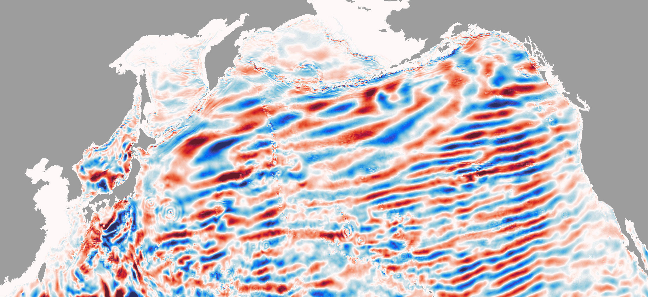
The 2019 NISKINe experiment included a broader variety of instruments and took place in a very different environment (Figure 1) than OSE. The background field in NISKINe is much more advective, and sampling efforts focused on smaller scales than during OSE. Inertial displacements (circles in the surface drifter tracks) are much more obvious in OSE than in NISKINe.
FIGURE 1. Maps of the (top) 1987 Ocean Storms Experiment (OSE) and (bottom) 2019 Near-Inertial Shear and Kinetic Energy in the North Atlantic Experiment (NISKINe), both showing similar 25-day observational periods and roughly 530 km × 330 km regions. The top panel is reproduced from D’Asaro et al. (1995), where tracks are from surface drifters and labeled dots indicate moorings. Twenty-five-day averaged SSHs (2 cm contours) are shown for the NISKINe experiment, along with the tracks of ship and instruments between May 25 and June 18, 2019. © American Meteorological Society. Used with permission. > High res figure
|
Wind Forcing
Wind forcing was substantially different during OSE and NISKINe (Figure 2a). Data during these experiments are available from in situ observations (D’Asaro et al., 1995; Klenz et al., 2022) and hourly 0.5° wind reanalysis (e.g., MERRA-2; Gelaro et al., 2017). Reanalysis wind stress is less accurate and slightly weaker than the in situ observations, but useful for forcing large-scale models.
During OSE, a well-defined 300 km diameter low-pressure system propagated northeast across the Pacific. On October 4, 1987, the storm passed slightly to the north of the OSE site, placing it in an ideal location for observing equatorward-propagating NIWs from the storm’s wake. In situ observations show a 1.5 Pa wind stress that veered from southerly to westerly over a 24-hour period. Following the storm, the wind stress remained around 0.1 Pa for 25 days, allowing the ocean to freely adjust to the storm (D’Asaro et al., 1995; Figure 2a).
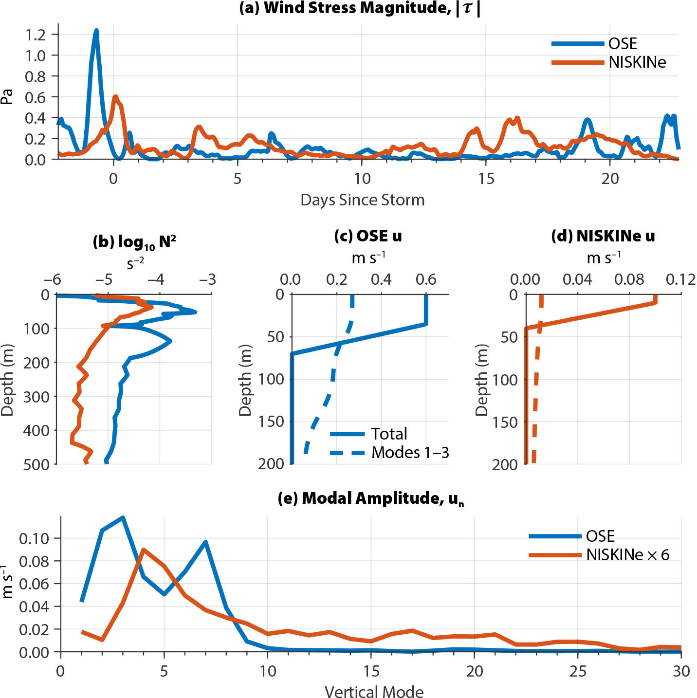
FIGURE 2. (a) MERRA-2 wind stress from OSE and NISKINe. WOA23 buoyancy frequency squared (b) was stronger in the upper ocean during OSE than during NISKINe. The initial zonal velocity was stronger and deeper during (c) OSE than during (d) NISKINe. The first three modes explain almost half of the mixed-layer current during OSE (c), but only 1/10th of the current during NISKINe (d). Modal amplitudes (e) peak around 10 cm s–1 for modes 1–7 and are much smaller for higher modes, especially during OSE (all modes were normalized to 1 at the surface). > High res figure
|
During NISKINe, a number of low-pressure systems originated off the coast of North America near 45°N and propagated northeast before hooking back to the northwest or dissipating. On May 30, 2019, in situ observations show that a storm reached the NISKINe site at 58°N, producing a 0.6 Pa westerly wind stress for about 12 hours (Thomas et al., 2020). This storm was smaller and shorter lived than the OSE storm, leaving a weaker and less spatially coherent near-inertial wake. A second storm passed the NISKINe site about 15 days later, disrupting the free adjustment of the ocean to the initial storm (Figure 2a).
The OSE and NISKINe events had similar maximum wind stress (1.5 Pa vs. 0.6 Pa), but the NISKINe storm had much weaker near-inertial wind stress. High-pass filtering the wind stress at 0.8f produces a 0.2 Pa signal during OSE and a 0.02 Pa signal during NISKINe (Figure 3a,b). As a result, the idealized model of D’Asaro (1995a) can reproduce the initial OSE mixed layer currents using a 2.3 Pa eastward wind stress for 12 h, but the NISKINe currents only require a 0.2 Pa eastward wind stress for 10 h.
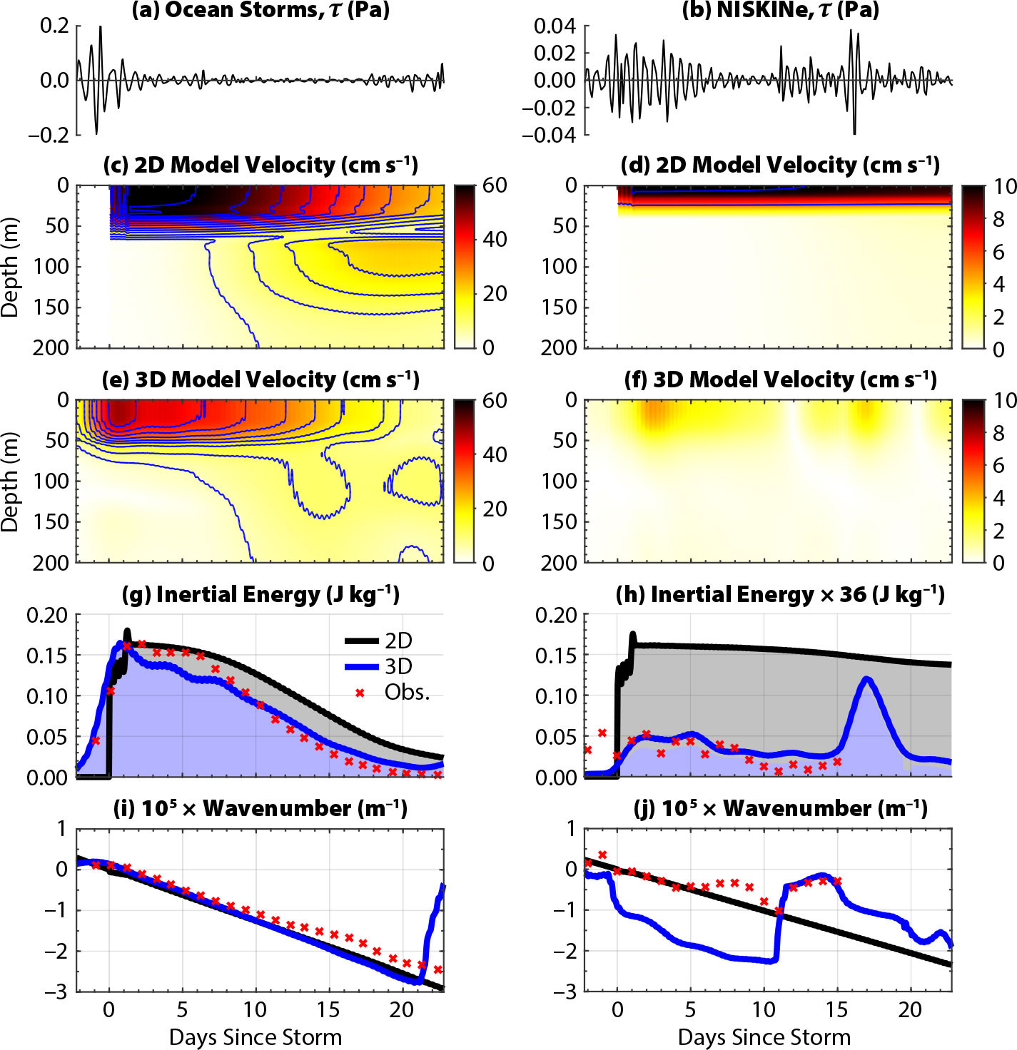
FIGURE 3. Zonal wind stress during OSE (a) is about six times larger than during NISKINe (b). Wind stress was high-pass Fourier filtered at 0.8f. Horizontal velocity in the 2D simulations evolves faster during OSE (c) than NISKINe (d). The 3D simulations (e and f) display different patterns than the 2D simulations. Plane-wave fits to mixed-layer velocity decay faster in OSE than in NISKINe (g and h), and both 2D simulations indicate linear wavenumber growth exactly consistent with β-refraction (i and j). Wavenumber growth is less clear in the 3D NISKINe simulation (j). Observations in (g) and (i) are digitized from D’Asaro et al. (1995) Figure 13. Observations in (h) and (j) are extracted from NISKINe drifter data (Figure 3) and shifted slightly in time to best align the simulations and observations. All velocities are back-rotated and smoothed over three inertial periods. The lines in (g) and (h) indicate total energy, while shading indicates energy in the plane wave fit, although the two are nearly indistinguishable. > High res figure
|
Vertical Structure of Initial Currents
The near-inertial currents directly following the storms (D’Asaro et al., 1995; Thomas et al., 2020) can be replicated by distributing the wind stress over the upper ocean with a body force that represents the vertical profile of the wind-stress divergence (D’Asaro, 1995a). This body force is uniform in the mixed layer and then decreases linearly through a stratified transition layer. OSE had a 35 m mixed layer and a transition layer from 35 m to 70 m (Dohan and Davis, 2011), while NISKINe had a 10 m mixed layer and a transition layer from 10 m to 40 m (Thomas et al., 2020).
Vertical modes are useful for analyzing NIWs because they are uncoupled when dynamics are linear, the mean flow is barotropic, and the bottom is flat. In such a setting, the initial velocity profile after a storm completely determines the vertical mode distribution of the near-inertial response (Alford, 2020). Here, we neglect local vertical-mode coupling during OSE and NISKINe because scattering by deep-ocean topography (Kelly et al., 2013; Mathur et al., 2014) and mesoscale currents (Dunphy et al., 2017; Savage et al., 2020) are typically quite weak.
The upper-ocean stress profile determines the vertical structure of the initial velocity profile following a storm (Pollard, 1970; D’Asaro et al., 1995). Background stratification, taken as the World Ocean Atlas 2023 (WOA23) monthly mean stratification (Figure 2b), determines the shapes of the vertical modes. The vertical mode amplitudes are then the projection of the initial velocity profiles onto each vertical mode. This process identifies more high-mode energy during NISKINe than during OSE (Figure 2a–c). OSE peaks at mode 2–3 (with a secondary peak at mode 7) and has almost no forcing above mode 10. In contrast, NISKINe peaks at modes 4–5 and has forcing out to about mode 30. These differences arise because the initial velocity was deeper and smoother (due to wind mixing) during OSE than during NISKINe, suppressing its projection onto high modes. In addition, high modes in the OSE region have slightly more curvature in the upper 100 m due to strong climatological stratification (Figure 2b), making them less useful for representing the smooth initial velocity profile. One exception is mode 7, which is preferentially excited during OSE because its shape nearly matches the initial velocity profile.
Near-Inertial Wave Propagation
In this section we discuss the effects of the gradient in the Coriolis parameter, β, and of the mesoscale relative vorticity, ζ, on the propagation of NIWs. At the simplest level, β and ζ shift the lowest frequency of the internal wave band. But β and ζ also alter the internal wave dispersion relation so that it contains spatially varying fields. These spatial inhomogeneities result in changes in wavenumber as NIWs propagate away from their generation sites. In the Wentzel-Kramer-Brillouin (WKB) limit, these variations in wavenumber result in ray curvature. This curvature, resulting from spatial inhomogeneity, is analogous to optical refraction (i.e., Snell’s law). Following an analogy made by Asselin et al. (2020), we refer to these internal-wave processes as β-refraction and ζ-refraction. Analyses of NISKINe and OSE are concerned with the evolution of the wave vector and wave propagation (both horizontal and vertical) and target refraction, not just the shift in the lowest frequency of the internal wave band.
β-Refraction
Drifter Observations
Following the passage of the OSE storm, D’Asaro et al. (1995) fit a plane wave to 36 drifters that were spread over 3° latitude (330 km) in the mixed layer. The southward wavenumber of the back-rotated near-inertial velocities increased linearly in time, precisely as predicted by β-refraction.
During the NISKINe field experiment in 2019, a total of 47 Surface Velocity Program (SVP), GPS-tracked drifters were deployed (Figure 4a). The number of drifters increased from about 13 at the peak of the storm event on May 30, 2019, to 47 over the course of the next 15 days. The drifter array extended over several hundred kilometers in the zonal and meridional directions, similar to the spread in OSE. In order to investigate whether β-refraction was present during NISKINe, a plane wave fit analogous to D’Asaro et al. (1995) was performed to drifter mixed-layer inertial currents back-rotated to the peak of the storm. Initial horizontal wavenumbers, phase, and amplitude of the plane wave excited by the storm were estimated through linear least squares. From these initial conditions, a nonlinear fit similar to D’Asaro et al. (1995) was performed. The resulting increase in southward meridional wavenumber was generally consistent with the expected rate of increase due to β-refraction (Figure 4b). However, contrary to OSE, where the increase in southward meridional wavenumber was almost perfectly described by β-refraction, continuous wind forcing and boundary effects during NISKINe likely caused deviations from β-refraction, which will be discussed further in the next section.
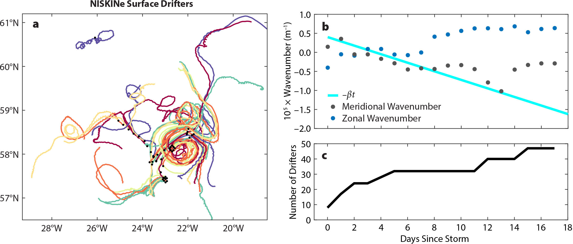
FIGURE 4. (a) Trajectories of surface drifters deployed during the NISKINe field experiment. Trajectories are colored at random and are shown between the peak of the storm on May 30, 2019, and June 16, 2019. Black dots indicate initial locations. (b) Plot shows meridional (black dots) and zonal (blue dots) wavenumbers resulting from a fit of back-rotated drifter near-inertial velocities to a plane wave solution. The cyan line indicates the expected decrease in meridional wavenumber due to β-refraction. (c) The graph shows number of drifters available for the plane wave fit. > High res figure
|
2D Simulations
D’Asaro (1995a) replicated the OSE drifter observations of β-refraction using a simple two-dimensional (2D) model without a mean flow. The model solved the hydrostatic, Boussinesq equations of motion using finite differences with 24 density layers and a 10 km horizontal grid oriented in the north-south direction (Price, 1983; D’Asaro, 1995a). D’Asaro (1995a) probed the model’s sensitivity to changes in wind forcing, nonlinearity, stratification, and viscosity. The results emphasized that β-refraction was incredibly robust while simultaneously highlighting the model’s failure to replicate the anomalously rapid decay of near-inertial energy.
Here, we configure an idealized 2D model like that of D’Asaro (1995a) to simulate β-refraction in both OSE and NISKINe in the absence of a mean flow. We use the Coupled-mode Shallow Water model (Kelly et al., 2021), which is linear and employs 128 vertical modes instead of 24 density layers. The initial velocity profiles are produced using an impulsive wind distributed vertically by a body force. The wind has a Gaussian meridional profile with a width of 300 km. The model is integrated for 30 days and run without damping or viscosity (the 4,000 km domain is large enough to prevent boundary reflections).
We analyze the simulations by back rotating the horizontal currents to the start of the respective storm (i.e., October 4, 1987, or May 30, 2019) and averaging them over three inertial periods (D’Asaro et al., 1995). Surface velocities are then fit to a cosine function along a meridional section within 200 km of the experimental site (D’Asaro, 1995a). In all cases, the cosine fit explains almost all meridional variance in the surface currents.
Mixed-layer energy decays in both 2D simulations as low modes propagate equatorward after the passage of the storm. The OSE results (Figure 3) are functionally identical to those of D’Asaro (1995a), confirming that the southward wavenumber grows linearly in time and that the escape of low modes explains the decay in mixed-layer energy after the storm. Simply subtracting the first three modes from the initial velocity profile replicates the downward propagation of energy in this simulation and development of a current minimum near 55 m depth (Figures 2c and 3c). Conversely, the NISKINe simulation displays little decay of mixed-layer energy or downward propagation (Figure 3d,h) because (1) the initial velocity profile is primarily composed of high modes, and (2) β-refraction occurs slightly slower at the higher latitude of NISKINe (58°N vs. 47.5°N). For example, subtracting the first three modes from the NISKINe profile does not greatly reduce mixed-layer energy (Figures 2d and 3d).
The preceding paragraph attributes the decay of mixed-layer energy to horizontal energy propagation, which causes the mode 1–3 amplitudes to decrease to approximately zero (under the storm), while high-mode amplitudes remain nearly constant. An alternative hypothesis for the decay of mixed-layer energy is that the vertical modes dephase without any modal amplitude decay, producing downward energy radiation. We examine this mechanism by rescaling the modes so that their amplitudes (but not phases) remain constant and re-compute the mixed-layer energy. Remarkably, the two mechanisms produce nearly identical energy decay in the mixed layer, indicating that dephasing and amplitude decay (through horizontal radiation) are equally effective in removing mixed-layer energy. However, the two decay mechanisms produce vastly different energy transfers to the deep ocean. When low-modes radiate horizontally (as seen in the OSE simulation), 90% of the initial mixed-layer energy is lost, but only 30% is transferred to the deep ocean (under the storm). If low modes simply dephased, the total energy under the storm would be conserved, and a 90% decay in mixed-layer energy would correspond to a 90% transfer to the deep ocean.
3D Simulations
Three-dimensional (3D) simulations improve on the 2D simulations by including spatially variable, time-dependent wind stress and incorporating interactions with coastlines (Kelly, 2019) and sloping topography (i.e., topographic scattering; Griffiths and Grimshaw, 2007; Kelly et al., 2021). Like the 2D simulations, these 3D simulations do not include a mean flow. The 3D simulations are conducted on a global 0.1° spherical grid with realistic topography and hourly reanalysis wind forcing. Only the eight lowest modes are included in these simulations to limit their computational expense. However, only these low modes are dispersive enough to propagate long distances and interact with coastlines and bottom topography. In contrast, the neglected high modes are hypothesized to primarily interact with the eddy field, which is absent in these simulations. The 3D simulations are integrated for 30 days and require numerical damping to both stabilize the model and limit currents in shallow water. The simulations use quadratic bottom drag and a horizontal viscosity of 100 m2 s–1. The wind stress is high-pass Fourier filtered at 0.8f to eliminate mean flows (e.g., Ekman transport). Because the model is linear, this process is equivalent to filtering the model output, which is typical in modeling studies of NIWs (e.g., Raja et al., 2022).
Snapshots of sea surface height (SSH) from the 3D simulations demonstrate the contrasting settings of OSE and NISKINe (Figure 5). Fifteen inertial periods after the OSE storm, SSH and horizontal velocity clearly exhibit a southward-propagating NIW with a 500 km wavelength (at 47.5°N). The SSH signal is approximately 1 cm, which is comparable to the internal tide and remarkably large considering NIWs are primarily composed of KE. In contrast, the NISKINe site is north of the mid-latitude storm tracks, so SSH is only 1 mm and does not display a prominent equatorward wave (Figure 5b).
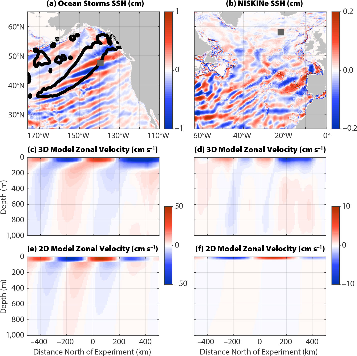
FIGURE 5. Sea surface height (SSH) displays large-scale equatorward propagating near-inertial waves 15 inertial periods after the OSE (a) and NISKINe (b) storms. Dark gray squares indicate experimental sites. Black contours indicate regions where wind stress exceeded 0.4 N m–2. (c and d) Meridional cross sections of zonal velocity in the 3D simulations indicate downward and equatorward wave propagation consistent with β-refraction. The 2D OSE simulation (e) is in close agreement with its 3D counterpart, while the 2D NISKINe simulation (f) bears little resemblance to its 3D counterpart. > High res figure
|
The 3D simulations have weaker mixed-layer velocities and are less energetic than the 2D simulations because they contain fewer vertical modes (i.e., 8 vs. 128). Horizontal viscosity and bottom drag also slightly reduce the energy in the 3D simulations, but this effect is almost an order of magnitude smaller than removing modes 9–128. The 3D OSE simulation is otherwise remarkably similar to the 2D simulation (Figures 3 and 5).
In contrast, the 3D NISKINe simulation bears little resemblance to its 2D counterpart. Mixed-layer velocities are very small (Figure 3f,h), and the wavenumber fit has a slope of β from 0 days to 10 days, but the intercept is less than zero (Figure 3j), suggesting β-refraction is occurring due to a previous storm (or remotely generated waves). The latter could be due to wave reflection or generation by coastlines because Iceland is only 500 km north of the site, or continuous wind forcing that creates a confused sea. The wavenumber also “resets” to zero during days 11–15, suggesting local NIWs are generated by a second storm. From these standpoints, the NISKINe site is less ideal for observing large-scale β-refraction than the OSE site. Despite these limitations, the NISKINe drifters clearly identify β-refraction (Figure 3h,j) that shows energy and wavenumber slopes similar to those in the 3D simulations. We note that expanding the fit region from 200 km to 300 km in the 3D model or sampling the 3D model along the observed drifter tracks greatly improves the agreement between the 3D model and observations in Figure 3j (not shown).
The NISKINe observations of energy are consistent with the 3D model (Figure 3h), which only has eight modes, rather than the 2D model, which has 128 modes. This fact suggests that the observed plane-wave fit is dominated by low modes. High modes may be missing from the plane wave fit because they are less dispersive and more susceptible to decoherence through ζ-refraction. Similarly, the OSE observations track the 2D simulation for days 1–7 but follow the 3D simulation more closely after day 10. This transition suggests that modes 9–128 (which are absent in the 3D simulation) play a lesser role in the observed plane wave fit over time.
ζ-Refraction
Apart from the wind-forcing, the NISKINe site may not be ideal for observing β-refraction because it is characterized by an active mesoscale eddy field capable of modifying NIWs on relatively small spatial and short temporal eddy scales. Thus, eddies obfuscate the smooth and slow distortion of NIWs by β-refraction. Unlike OSE, NISKINe used observational strategies designed to sample these small scales. For example, one ship-based survey consisted of loops, each completed in a fraction of an inertial period, that encircled the approximately 10 km wide axial jet of a dipole vortex (Figure 6a). By rapidly sampling the cyclonic and anticyclonic sides of the jet over several inertial periods, the goal was to measure differences in wave phase across the jet and compare their evolution to the theoretical prediction for ζ-refraction (Asselin et al., 2020; Thomas et al., 2020).
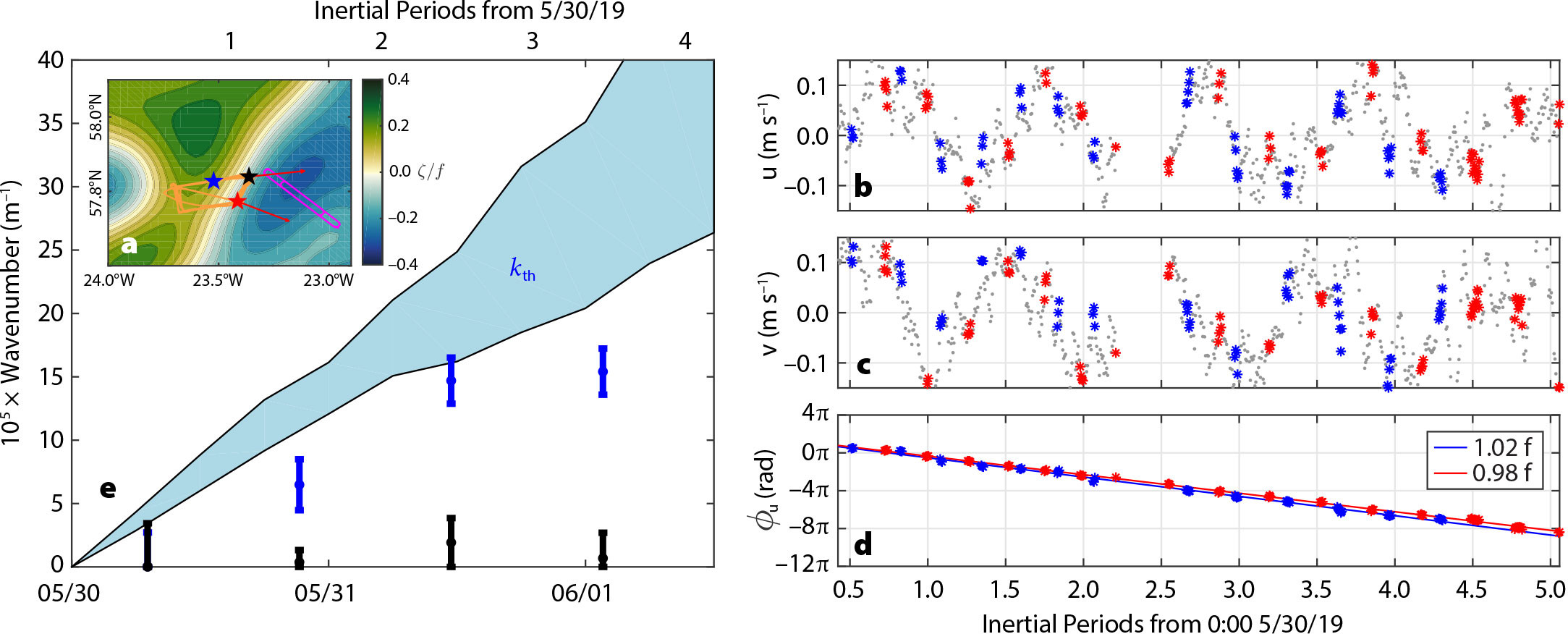
FIGURE 6. Evidence of ζ-refraction observed during the NISKINe survey that was collected shortly after the passage of a storm on May 30, 2019. (Inset, a) The survey (orange line) straddled the axial jet of a dipole vortex (vorticity normalized by f is shown in color). Time series of the velocity anomaly (made with respect to the nearly-barotropic flow below 50 m) are shown in the (b) zonal and (c) meridional directions, averaged over the upper 40 m. The velocities measured at all points during the survey are indicated by gray dots, while data for the blue and red asterisks were collected from the locations marked by the blue and red stars in (a) on either side of the jet. (d) The angle that the velocity anomaly vector makes with the horizontal, Φu, a measure of wave phase, at these two locations decreases with time at a slightly faster (slower) rate on the cyclonic (anticyclonic) side of the jet. (e) The lateral gradient in Φu, an estimate of the wave vector, in the cross-jet direction (blue dots with error bars) increases at a rate consistent with the theoretical prediction for ζ-refraction (blue shading) for the first 2.5 inertial periods. In contrast, the gradient in Φu in the along-jet direction (black dots with error bars) is near zero through the time series. Figure adapted from Thomas et al. (2020). > High res figure
|
The survey was conducted shortly after the May 30, 2019, passage of a storm that accelerated inertial motions. Velocity anomalies in the upper 40 m were characterized by a clean near-inertial signal that rotated clockwise with time (Figure 6b,c). The rate of rotation of the velocity vector was measurably faster (slower) on the cyclonic (anticyclonic) side of the axial jet, and thus generated a lateral difference in wave phase (Figure 6d). Dividing the phase difference by the spacing between the anticyclonic and cyclonic sides of the jet where the velocities were measured (indicated by the red and blue stars in Figure 6a) yields an estimate for the wave vector in the cross-jet direction (Figure 6e). Similarly, the wave vector in the along-jet direction can be estimated from two locations along the jet (i.e., the red and black stars in Figure 6a), resulting in values that are not significantly different from zero (Figure 6e). In contrast, the inferred wave vector in the cross-jet direction grows, and for the first about 2.5 inertial periods increases at a rate that is consistent with the theoretical prediction for ζ-refraction estimated using the observed vorticity gradient of the axial jet (see Figure 6e).
The rate of change of the wave vector is two orders of magnitude larger than what β-refraction would yield (cf. Figure 3j), implying that ζ-refraction is the dominant process setting the wave vector on smaller scales. Having said this, when diagnosed over the O(100 km) width of the drifter array (which sampled the axial jet of the dipole vortex early in the drift) and for long times, β-refraction has skill in predicting the meridional wave vector (e.g., Figure 4b), suggesting that variations in phase caused by ζ-refraction average out in the plane wave fit to the back-rotated velocities when calculated on large enough scales. Conversely, this indicates that the method of using plane wave fits to drifter velocities collected over O(100 km) length scales and tens of days is not well suited for detecting NIW phase differences generated by ζ-refraction.
Damping of Near-Surface Inertial Motions by Near-Inertial Wave Radiation
While the meridional wavenumber inferred from the plane wave fit is consistent with β-refraction, the NIW radiation that is predicted by theory only partially explains the observed decrease in mixed-layer inertial KE in OSE (e.g., Figure 3g). During the NISKINe survey, the mixed-layer inertial motions also exhibited a drop in KE; however, this can be fully explained by NIW radiation that, in this case, is attributable to ζ-refraction.
During the NISKINe survey, between 2.5 and 5 inertial periods after the passage of the storm, the mixed-layer inertial KE decreased by a factor of two (Figure 7c). A towed profiler that was deployed during this period measured about 10 m undulations in surfaces of constant density (or isopycnals) beneath the mixed layer (Figure 7a). The isopycnals were oscillating at a near-inertial frequency, a telltale sign of inertial pumping, that is, vertical velocities at the base of the mixed layer driven by convergence/divergence of inertial motions (Gill, 1984). Such isopycnal displacements set up pressure anomalies which, when correlated with the near-inertial velocities, generate a wave energy flux and NIW propagation. Pressure and velocity correlations were calculated to quantify the vertical and horizontal components of the energy flux (for more details, see Thomas et al., 2023). The direction of the horizontal energy flux and hence NIW propagation (indicated by the red arrows in Figure 6a) points toward the region of anticyclonic vorticity, while the vertical energy flux is downward and thus drains the mixed layer of near-inertial KE. Moreover, the magnitude of the vertical energy flux is strong enough to explain the observed drop in KE, within the 95% confidence interval of the estimate (Figure 7c).
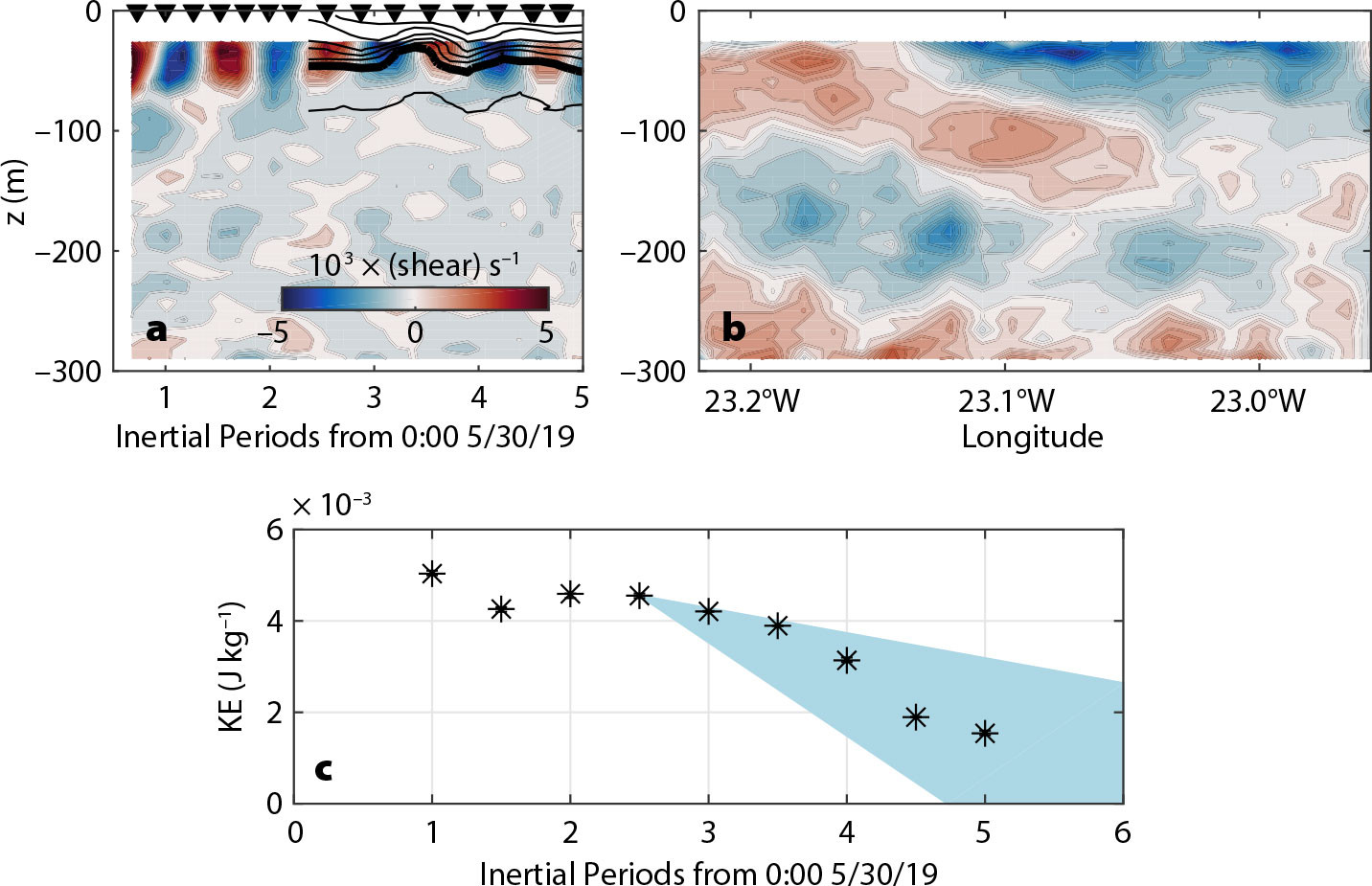
FIGURE 7. Evidence of vertical radiation of near-inertial waves (NIWs) and the resultant damping of inertial motions in the mixed layer during NISKINe. (a) Vertical shear of the meridional velocity and potential density measured at the location indicated by the red star in Figure 6a. Isopycnals are contoured every 0.05 kg m–3 with the thick contour denoting the 27.15 kg m–3 isopycnal and the triangles indicating the times when the location was sampled. (b) A transect of the vertical shear of the meridional velocity along the magenta track shown in Figure 6a made 6.6 inertial periods (3.9 days) after 0:00 5/30/2019 showing an NIW propagating down and to the east. (c) Time series of near-inertial kinetic energy (KE) in the upper 50 m (black stars). The reduction in KE after 2.5 inertial periods is similar to the drop in energy calculated from the vertical energy flux estimated from the observed inertial variations in density and integrated in time starting at 2.5 inertial periods (blue shading, which spans the 95% confidence interval of the estimate). Figure adapted from Thomas et al. (2020) and Thomas et al. (2023). > High res figure
|
The energy flux calculation suggests that the NIW was propagating down and into the anticyclone, a behavior that is consistent with the theory of ζ-refraction and is a phenomenon that has been referred to as an inertial chimney (Lee and Niiler, 1998) or an inertial drainpipe (Asselin and Young, 2020). Indeed, a section that transected the western edge of the anticyclone revealed a pattern in shear consistent with an inertial chimney/drainpipe, namely a beam of NIW shear was directed down and to the east into the anticyclone (Figure 7b). The section was made 6.6 inertial periods (3.9 days) after the passage of the storm, which is a sufficient amount of time for the NIW to have propagated 130 m below the transition layer (a depth similar to the vertical extent of the beam on the section), given the estimated group velocity of the wave (e.g., Thomas et al., 2020).
A beam of NIW energy was also observed in OSE. Velocity profiles from moorings in the beam showed a maximum in near-inertial KE that descended about 100 m in 20 days (D’Asaro et al., 1995). Contrasting this with the downward propagation of the NIW in the NISKINe survey, it is clear that ζ-refraction can greatly amplify NIW radiation and the damping of mixed-layer inertial motions relative to β-refraction. In fact, even a modest amount of ζ-refraction associated with weak vorticity gradients might explain why the observed damping of mixed-layer inertial motions in OSE was more rapid than that predicted by β-refraction (e.g., Figure 3g). Indeed, Balmforth and Young (1999) reported that they could capture the observed more rapid decay in OSE using an idealized model for NIWs on a β-plane in a geostrophic flow with a vorticity gradient of the same magnitude as β (for comparison, the vorticity gradients in the NISKINe survey were O(100) times larger than β).
Discussion
Although the vorticity gradients in the Northeast Pacific are weaker than those in the North Atlantic, they are up to 10 times larger than β. Thus, it is puzzling that no clear modulations in the phase of mixed-layer inertial motions with vorticity were observed in OSE (D’Asaro, 1995b). This is in contrast to NISKINe where variations in NIW phase resulting from ζ were conspicuous. Using the results from the analyses described above and NIW-mean flow interaction theory, we attempt to solve this apparent conundrum.
Part of the answer is that the method used by D’Asaro et al. (1995) to infer phase differences in inertial motions, that is, a plane wave fit to back-rotated drifter velocities distributed over several degrees of latitude and spanning a few weeks, is not well suited for measuring ζ-refraction. This was certainly the case for NISKINe. For example, if the mixed-layer inertial velocities in NISKINe had only been measured with drifters, it may have been concluded that lateral variations in phase are primarily caused by β-refraction, similar to OSE. However, with the modern-day capabilities of surveying velocity and density fields at high-resolution, NISKINe was able to demonstrate that on smaller spatial and temporal scales, ζ-refraction is in fact dominant and leads to the rapid radiation of near-inertial energy out of the mixed layer.
Having said this, significant differences in the stratification and vertical structure of the NIW fields in the two regions imply that NIWs in the Northeast Pacific should be less affected by vorticity than those in the North Atlantic. Hence, the apparent dominance of β-refraction over ζ-refraction in OSE may not solely be an artifact of the analysis technique. These dynamics can be understood using the framework of the YBJ equation (Young and Ben-Jelloul, 1997), which describes the evolution of the amplitude and phase of NIWs in an eddy field. For a summary of the YBJ equation, see Box 1.
The YBJ equation can be used to quantify the competition between ζ-refraction and dispersion. NIW dispersion decreases with mode number and increases with stratification. The mixed layer at the NISKINe site is only 10 m deep, and wind forcing excites modes as high as n = 30, with peak energy in modes 4 and 5 (see Figure 2). In OSE, the energy peaked in modes 2 and 3, and there was very little energy in higher vertical modes. This difference is compounded by the comparatively weak NISKINe stratification (see Figure 8a for a comparison between Rossby radii and modal dispersivities, ℏn = f0 Rn2, at the two sites). The first Rossby radius, R1, at the NISKINe site is 12.9 km while that at the OSE site is 26.4 km. For higher vertical modes, OSE Rn is approximately 2.5 times larger than NISKINe Rn. NIW dispersion, quantified by the modal dispersivity ℏn in Figure 8b, is smaller by a factor of 5.5 at the NISKINe site than at the OSE site.
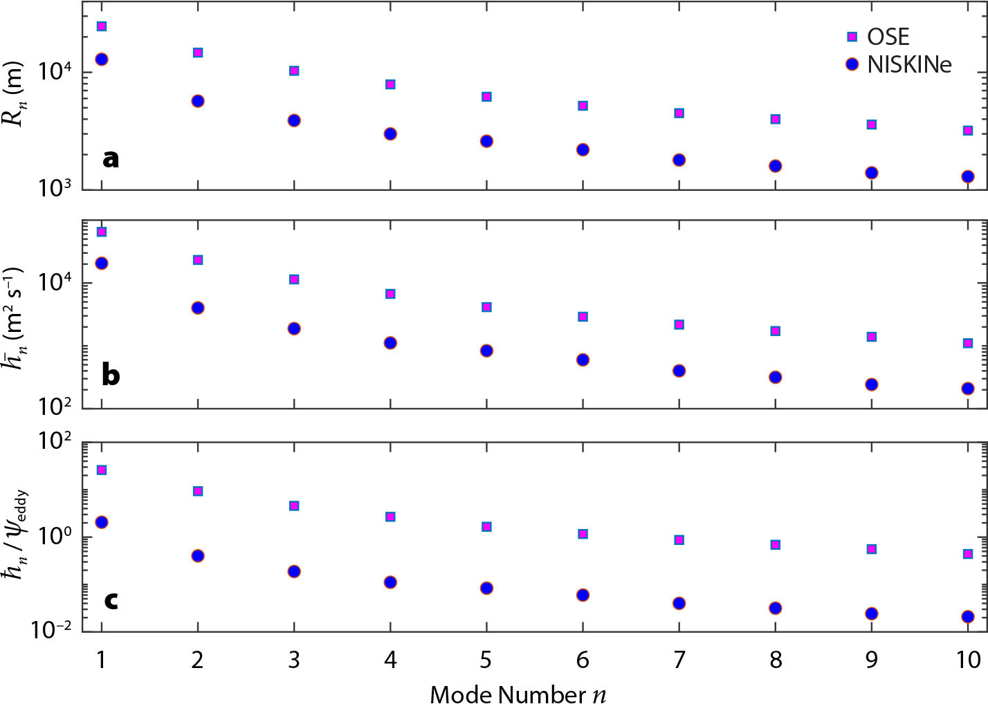
FIGURE 8. Panel (a) compares Rossby radius Rn in meters at the OSE site with Rn at the NISKINe site. With n ≥ 2, the OSE Rn is approximately 2.5 times the NISKINe Rn. Panel (b) compares the model dispersivities ℏn = f0Rn2 at the OSE site to those at the NISKINe site. With n ≥ 2, OSE ℏn is approximately 5.5 NISKINe ℏn. Results are based on climatological stratification from World Ocean Atlas 23. Panel (c) compares the non-dimensional parameter in Equation 5 at the two sites. The disparity between OSE and NISKINe in panel (b) is increased because the NISKINe Ψeddy is four times larger than the OSE Ψeddy. For the same mode number n, the non-dimensional parameter ℏn/Ψeddy is larger by a factor of at least 20 in OSE than in NISKINe. > High res figure
|
The dispersive term in the YBJ equation (i.e., the horizontal Laplacian of A in Equations 2 and 4) opposes the development of small scales in the NIW field. Because of the very different dispersivities and modal projections, this opposition is more effective in OSE than in NISKINe. Thus, the high-mode excitation in NISKINe is strongly imprinted with eddy scales. This imprinting is less effective in OSE.
Moreover, eddies are significantly weaker in OSE than in NISKINe: the magnitude of the geostrophic streamfunction associated with eddies in NISKINe, estimated from objective maps of the horizontally non-divergent flow field, is Ψeddy = O(104 m2s–1). In OSE the vorticity of the mesoscale eddy field is O(10–6 s–1) and the eddies are about 50 km in diameter (e.g., Figure 3 in D’Asaro, 1995b). Thus, in OSE, Ψeddy = O(2,500 m2s–1)—one quarter that of NISKINe. This factor of four in the strength of the eddies further compounds the differences between OSE and NISKINe.
The non-dimensional parameter that controls the strength of dispersion relative ζ-refraction is the ratio ℏn/Ψeddy in Equation 5. Because OSE Ψeddy is about one quarter that of NISKINe Ψeddy, the non-dimensional ratio ℏn/Ψeddy is over 20 times larger in OSE than in NISKINe (see Figure 8c). Energy containing OSE modes n = 1, 2, and 3 have ℏn/Ψeddy equal to 26.0, 9.3, and 4.6, respectively. Thus, these energy-containing OSE modes are strongly dispersive relative to the local eddy field. It is not until n = 7 that OSE ℏn/Ψeddy is less than one. But there is little energy in these weakly dispersive high-n OSE modes (see Figure 2e).
In NISKINe, however, ζ-refraction should dominate over dispersion (ℏn/Ψeddy < 1) for modes with n ≥ 2: NISKINe modes n = 1, 2, and 3 have ℏn/Ψeddy equal to 2.1, 0.40, and 0.2, respectively. These considerations provide a physical explanation for why there was no observational evidence of ζ-refraction in OSE, while it was on clear display in NISKINe.
Conclusion
The key lesson to be learned from our analyses contrasting the behavior of NIWs in the North Atlantic and the Northeast Pacific is that the sensitivity of NIWs to vorticity is not simply a function of the strength and structure of the vorticity field. It also depends critically on the stratification and modal distribution of near-inertial energy. In particular, for a given eddy field, NIWs are more sensitive to vorticity in regions with weaker stratification and wind forcing that injects energy into higher modes, like the North Atlantic in late spring/early summer. This finding implies that damping of mixed layer inertial motions by NIW radiation depends on stratification, modal content, β, and vorticity in ways that can be unexpected, although entirely consistent with the NIW-mean flow interactions described by the YBJ equation (see Rocha et al., 2018, and Asselin et al., 2020, for additional examples). In particular, the dependence on modal content does not always follow the commonly used rule of thumb that higher modes radiate more slowly than lower modes. Because higher modes are more susceptible to ζ-refraction, they can radiate energy more rapidly than lower modes under certain circumstances. This was exemplified in the NISKINe survey highlighted here, where it took only three days (five inertial periods) for the mixed-layer inertial KE to decrease by a factor of two, in contrast to 12 days in OSE (cf. Figures 3g and 7c), in spite of the fact that the NIWs in NISKINe had higher mode numbers than the waves in OSE (Figure 2e).
The rate at which mixed-layer inertial motions are damped affects how much KE is (1) injected into the ocean by winds, (2) radiated into the interior, and (3) available for mixing. Global estimates of the wind-work and NIW energy fluxes to the deep ocean are uncertain. Understanding and quantifying the sensitivity of the damping rate to the parameters that set the efficacy of NIW radiation could help improve these estimates and should be studied in regions in addition to the North Atlantic and Northeast Pacific described here.
Acknowledgments
We are grateful to the captain and crew of R/V Neil Armstrong who made the collection of the NISKINe observations possible. This work was supported by ONR grants N00014-18-1-2798 (LNT), N00014-181-2800 (SMK), N00014-18-1-2780 (LR), N00014-18-1-2445 (V H), N00014-18-1-2386 (TK), N00014-18-1-2386 and N00014-22-1-2585 (HLS) and N00014-18-1-2803 (WRY) under the NISKINe Departmental Research Initiative. The NISKINe drifters used in this study were funded by ONR grant N00014-17-1-2517 and NOAA grant NA150AR4320071 “The Global Drifter Program.”