Introduction
Submersible, or in situ, fluorometers are devices used in freshwater and marine environments to measure the presence of compounds (fluorophores) that fluoresce when exposed to specific wavelengths of light. These measurements can be used, for example, as indicators of water quality, contamination, and flow dynamics. The earliest submersible fluorometers (Wheaton et al., 1979) were designed with a single channel (i.e., measuring fluorescence at a specific wavelength while rejecting the rest of the spectrum). However, the presence of multiple fluorescent species in natural waters makes it sometimes challenging to attribute the measured signal to a single compound with certainty due to spectral overlap, so multichannel fluorometers have been employed more recently.
Climate change and its associated impacts are increasing the demand for high-resolution monitoring of the environment using optical sensors that enable fast detection and are small enough to be integrated into mobile platforms. For example, harmful algal blooms (HABs) can cause billions of dollars in direct damages to fisheries (Davidson et al., 2020) and fishery-dependent communities (Weir et al., 2022), and reduce the socioeconomic value of recreational areas (Mardones et al., 2020). Preventative and mitigative actions can be taken if warning signs, such as the concentrations of the fluorophores chlorophyll a (Chl-a) and phycocyanin (PC) (Shen et al., 2012), are monitored and detected early (Davidson et al., 2020). In another example, the assessment of marine carbon dioxide removal strategies, such as point-source oceanic alkalinity enhancement, requires a careful understanding of the near-field dynamics that are studied using dye tracer experiments (Fennel et al., 2023). These experiments use fluorescent rhodamine water tracer (RWT) dye to make spatio-temporal measurements of dye plume dispersion. In another example, petroleum-derived contaminants such as crude oil can be detected using ultraviolet fluorometry. Overall, the scope and scale of human activity put enormous pressure on the global ocean and waterways, thus warranting the development and improvement of autonomous sensors, including fluorometers, for improved monitoring and response.
Access to this technology as well as to the education required to take advantage of it, both currently dominated by high-income countries, is a challenge recognized by the United Nations Decade of Ocean Science for Sustainable Development (2021–2030) (Harden-Davies et al., 2022). The current price of relevant industrial, single channel, in situ fluorometers is $3,400–$7,800 USD (Park et al., 2023). Industrial multichannel systems such the three-channel RBRtridente (RBR Ltd., Ottawa, Canada), Turner C3 (Turner Designs, San Jose, CA), or ECO Puck (Sea-bird Scientific, Bellevue, WA) have price and performance characteristics comparable to the single channel devices on a per-channel basis. To improve access and the use of sensor technology, the documentation on some oceanographic devices, their construction, use, and handling have been released to the public as open source (Butler and Pagniello, 2021; see also https://tos.org/diy-oceanography for additional open-source instrument projects published in Oceanography).
Open-source/DIY fluorometers exist in the ocean sciences space, with Chl-a fluorometers and “fluorometry-like” turbidity (Matos et al., 2020) and backscattering sensors (Downing, 2006) being popular. Costs are low in most instances, though two trends are noticeable. Either fluorometers tend to exhibit detection limits of 0.1 μg L–1 (or 0.1 ppb) or higher (Leeuw et al., 2013; Attivissimo et al., 2015; Park et al., 2023), which is at least one order of magnitude worse than industrial sensors (Park et al., 2023), or higher performing devices are configured as benchtop units (Truter, 2015) and have not made the sacrifices necessary to package the technology into a form capable of in situ deployment. The task of maintaining optical and electrical performance in a small, water-tight, pressure-safe housing is not trivial, and making concessions on size/mass rules out some of the most attractive use-cases of low-cost in situ fluorometers (Dever et al., 2020; Park et al., 2023). Thus, there is a gap in extant sensors between the advantages provided by open-source in situ sensors and the performance provided by industrial in situ fluorometers.
With this gap in mind, we introduce the PIXIE, a low-cost, open-source, four-channel in situ fluorometer. In lab testing, the PIXIE performs fluorometry with precision and accuracy comparable to the sensors available on the market. The default-configuration PIXIE can be assembled for $1,392.75 USD with one equipped channel. Each addition channel costs $525.25 USD, for an average of $742.13 USD per channel when the instrument is fully equipped.
For our work, a PIXIE unit was calibrated to demonstrate a limit of detection (Arar and Collins, 1997; Sieben et al., 2010) of 0.01 ppb RWT over a range 0 to ~60 ppb. The same unit was calibrated to demonstrate a limit of detection of 0.02 ppb Chl-a over a range of 0 to ~80 ppb. Deployed as part of a dye tracer experiment in Halifax Harbor, Canada, (see Figure 1) to study the near-field dispersion of RWT added to the cooling outfall of the Tufts Cove Power Generation Station, the PIXIE was configured to capture both RWT and Chl-a profiles, demonstrating its multichannel functionality. The in situ data were checked against discrete water samples collected in conjunction with the profiling to assure quality, demonstrating how this low-cost, open-source technology could assist in solving complex oceanographic tasks.
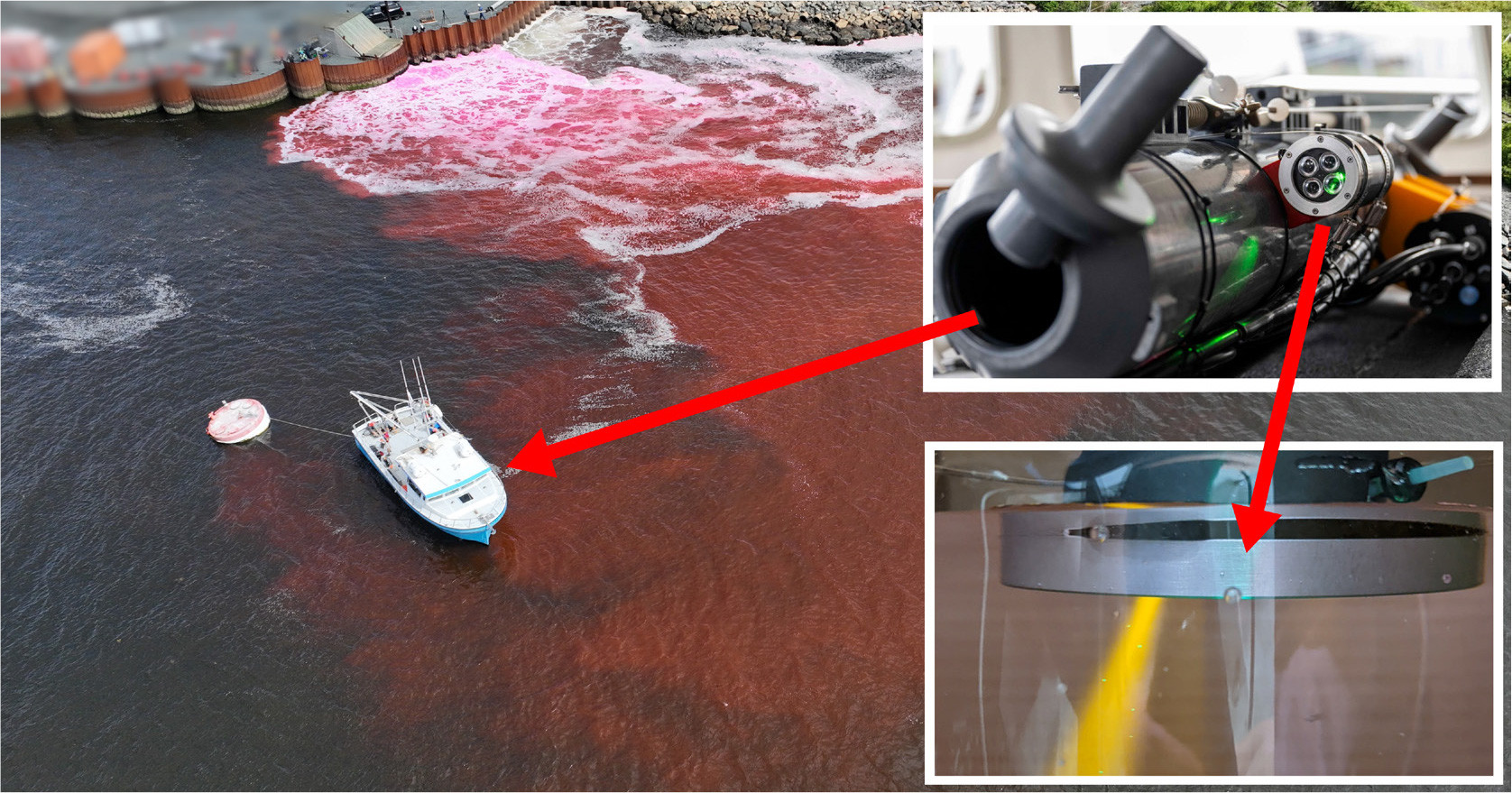
FIGURE 1. Drone photograph of the August 2023 Halifax Harbor tracer release experiment conducted from the diving vessel Eastcom. Insets: The PIXIE open-source fluorometer is shown mounted to the side of a Niskin bottle (top) and during rhodamine water tracer (RWT) calibration (bottom) in the lab. > High res figure
|
Materials and Methods
Open-Source Fluorometer
The materials needed to assemble a PIXIE are available on GitHub (https://github.com/KylePark0/PIXIE/tree/main), and fall into one of three categories: documentation, firmware, or hardware. The documentation includes a comprehensive user guide that details the design, assembly, calibration, and operation of the device. Bills of materials (BOMs) are provided for the mechanical and optical hardware, including vendors, and the electrical BOM comes pre-packaged to fabricate with PCBWay (PCBWay, Hangzhou, China). The listed optics include the components needed to assemble any of five presets: PC, phycoerithrin (PE), RWT, Chl-a, and crude oil. CAD models for every component, including machined and 3D-printed parts, are included. A rendering of the PIXIE with some dimensions (see Figure 2) is provided, in both normal and exploded views.
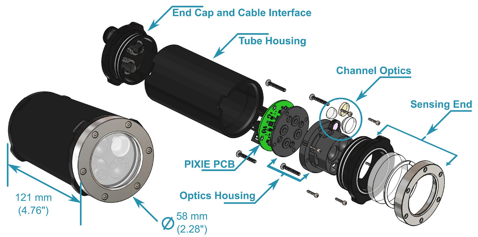
FIGURE 2. The PIXIE, in assembled view (left) and in labeled exploded view (right). For clarity, only one channel is populated with optics. Cable, excitation LEDs, and some O-rings are omitted. > High res figure
|
The PIXIE can be powered using a range of 5–20 V. It communicates with an external terminal or datalogger via RS-232, while drawing an average of 45 mA during active measurement (225 mW). Using a dedicated 12 V lithium-ion cell with a nominal capacity of two ampere-hours, the PIXIE can be expected to measure for 40 hours in 4°C waters. Its off-the-shelf components are rated for depths of at least 500 m. The housing is composed of anodized aluminum and borosilicate glass, allowing it to withstand a range of solvents used in laboratory calibration of fluorometers. Acetone is used to prepare standards of Chl-a (Arar and Collins, 1997), a nearly-neutral phosphate buffer solution (PBS) is used for solutions of PC (Jaeschke et al., 2021) and PE (Ardiles et al., 2020), and deionized water is used for RWT. The PIXIE is compatible with the above solvents but cannot tolerate the sulfuric acid that dissolves quinine sulfate, the stand-in for crude oil calibration. Sulfuric acid is used almost exclusively in literature to prepare fluorescence standards of quinine sulfate (Kristoffersen et al., 2018).
Sensor Design
Design notes for the PIXIE, available in the PIXIE Complete User Guide document provided at the GitHub link, are described briefly here for context. The PIXIE was designed with a focus on user configurability, and customization if desired. Users can simply acquire the hardware and assemble the default configuration or use the PIXIE’s documentation if more detailed customization is needed.
The PIXIE performs fluorometry using standard optics through an O-ring-sealed glass window. The user configures the targeted fluorophore for each of the four channels by selecting the appropriate optical filters and excitation LEDs. The PIXIE described in this work was equipped with hardware to target PC, RWT, Chl-a, and crude oil, though only the RWT and Chl-a channels were used. The PIXIE cannot measure using more than one channel at a time, but it can cycle between channels fast enough to achieve quasi-simultaneous measurements.
To extract only the fluorescence excited by the device itself, the PIXIE modulates the brightness of its excitation LEDs sinusoidally. While the change in brightness is imperceptible to the eye, the resulting fluorescence will have a synchronous brightness that can be distinguished from other sources of light. This allows PIXIE measurements even in bright laboratory or sunlit outdoor conditions. The process of measuring the sinusoidal fluorescence and converting it to a measure of fluorophore concentration, or lock-in amplification, is implemented digitally and can therefore be adjusted by more technically inclined users. The PIXIE detects the sinusoidal fluorescence using an AC-coupled transimpedance amplifier with a software-configurable gain of 400 MΩ, within a sample volume of 0.1 mL. More technical details can be found on our GitHub page.
Calibration
The PIXIE’s RWT and Chl-a channels were calibrated in the laboratory using a set of temperature-controlled standards. Fluorescence is known to depend strongly on temperature (Smart and Laidlaw, 1977), so the PIXIE was calibrated across a range of temperatures and concentrations. The set of temperatures and RWT concentrations were chosen to parallel previous work in this area (Park et al., 2023) for comparison’s sake. The protocols used were adapted from a US Environmental Protection Agency Method 445 on Chl-a fluorometer calibration (Arar and Collins, 1997). An effort was made to adapt the protocol to keep the number of expensive lab instruments and equipment to a minimum, though the protocol applied to Chl-a required a fume hood. The PIXIE was suspended above a beaker such that its sensing end was submerged without overflowing or trapping air bubbles (see Figure 1, bottom inset). A complete description of the calibration protocols is available in the PIXIE Complete User Guide document on GitHub.
Field Deployment
A 10 L Niskin bottle (General Oceanics, Miami, FL, USA) was prepared for use during an RWT tracer release experiment in Halifax Harbor, as depicted in Figure 1. The bottle was equipped with a proprietary datalogger that powered an array of external sensors, including for temperature and depth. The PIXIE was also mounted to the Niskin bottle, pointed downward, and constantly streamed its fluorometry data to the logger via the RS-232 protocol at a frequency of 16 Hz.
On August 10, 2023, a pre-set amount of RWT was released from the Tufts Cove Power Generation Station to study the dye plume. Multiple sensors and techniques were used, including the PIXIE-integrated Niskin bottle and an ecoCTD (Dever et al., 2020) equipped with a Cyclops-7F rhodamine fluorometer (Turner Designs). Discrete water samples were later analyzed in the laboratory using a benchtop fluorometer. The Niskin bottle was lowered into the water column and triggered at depths ranging from 0.5 m to 45 m. The sampling was conducted on a release day, a pre-release day (1 day prior) and a post-release day (1–3 days later). The PIXIE captured the vertical RWT/Chl-a concentration profiles to demonstrate its multichannel functionality, while the Niskin bottle provided a ground-truth measurement of the RWT concentration at the surface and above the seafloor. Data collected by each method were used to semi-quantitatively validate the performance of the PIXIE as an in situ fluorometer.
Results and Discussion
Calibration
A total of 37 data points was collected during the calibration of the PIXIE’s RWT channel. These consisted of six standard concentrations across six temperature setpoints. The 60 ppb measurement at 5°C saturated the device. A replacement 6.9°C temperature set point was also collected. A total of 37 data points were collected during the calibration of the Chl-a channel. The 80 ppb measurements at 5°C and 8°C saturated the device. A replacement 9.6°C temperature set point was also collected.
The raw fluorescence data for each data point were collected at the PIXIE’s maximum sample rate of 16 samples per second. In line with previous work (Park et al., 2023), the raw data were downsampled through a moving average of 16 samples, for an effective sample rate of 1 sample per second. Fifteen minutes of raw data were collected for each data point. During the last five minutes, 300 samples were collected, and the mean of these 300 samples was taken as the calibration data point. The prior 10 minutes of data were inspected to ensure an apparent equilibrium fluorescence had been reached.
The six standard concentrations for each fluorophore were used to generate a best-fit line for each temperature (see Figure 3). In the 60 ppb RWT case, a 5°C data point was first extrapolated from the six unsaturated temperature set points (6.9°C as well as the original five). In the 80 ppb Chl-a case, 5°C and 8°C were first extrapolated from the five unsaturated temperature set points (9.6 °C as well as the original four). The parameters of the resulting curves do not change significantly between the inclusion or exclusion of the extrapolated points. The coefficient of determination (R-squared) for each calibration curve exceeded 0.99 for RWT and 0.98 for Chl-a.
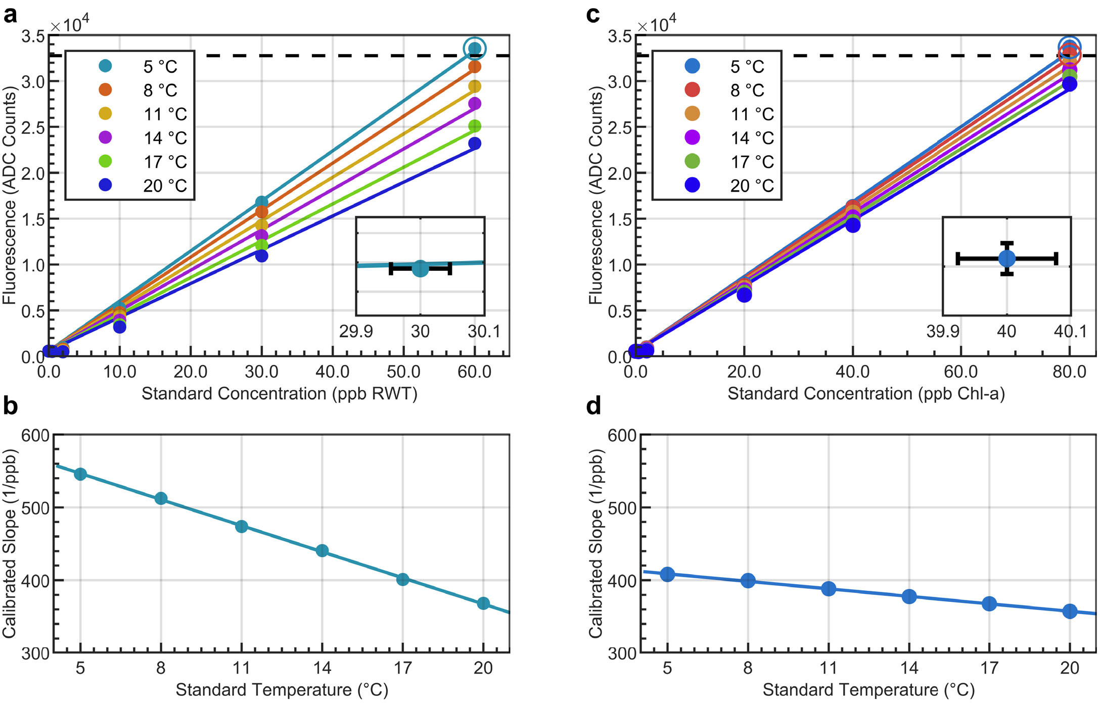
FIGURE 3. (a) Rhodamine water tracer (RWT) calibration curves, with a dashed line indicating saturation. The extrapolated point is encircled. Inset: Plot with concentration-equivalent 10-sigma error bars. (b) RWT temperature compensation “slope of slopes” curve. (c) Chl-a calibration curves, with a dashed line indicating saturation. Extrapolated points are encircled. Inset: Plot with concentration-equivalent 1-sigma error bars, illustrating sensitivity to bubbles. (d) Chl-a temperature compensation “slope-of-slopes” curve. > High res figure
|
To compensate measurements for the temperature of the sample volume, the slopes of each fit line are plotted, and a best-fit line is calculated. From the parameters of this fit, the all-cause temperature exponent can be approximated. The PIXIE achieved an approximate temperature exponent of –0.019°C–1 for RWT, consistent with previous results (Park et al, 2023). For Chl-a, the approximate temperature exponent obtained was –0.008°C–1, which is consistent with equivalent temperature parameters for Chl-a from the literature (Watras et al., 2017). The coefficient of determination for these curves exceeded 0.99.
The standard deviation of each 0 ppb (blank) data point was calculated. Applying the calibration curves to these blank standard deviations, the limit of detection was taken as three times the worst-case standard deviation across blanks. The limits of detection were found to be 0.01 ppb for RWT and 0.02 ppb for Chl-a. The upper limit of the PIXIE’s RWT detection range was found to be 58.9 ppb at 5°C, whereas it was 87.7 ppb at 20°C. For Chl-a, the upper limit of the detection range was found to be 78.8 ppb at 5°C, whereas it was 90.2 ppb at 20°C. Further details about these results can be found in the PIXIE Complete User Guide on at the GitHub link. Bubbles were observed during two of the 40 ppb Chl-a calibration trials, resulting in anomalously high standard deviations in those data sets as the bubble periodically stirred through the sample volume. The inset plot of Figure 3c illustrates 1-sigma error bars on the 40 ppb, 5°C data point. This contrasts with the 10-sigma error bars on the 30 ppb, 5°C RWT data point illustrated in the inset plot of Figure 3a.
To directly compare the cross-sensitivity of the two channels to the opposite fluorophore, the PIXIE’s RWT channel measured a standard of Chl-a and vice-versa. A complete description of the comparison and its results (Figure S1) is available in the online supplementary materials.
Field Deployment
Figure 4 depicts the first deployment of the PIXIE in August 2023 during the dye tracer release experiment. Three key stations’ worth of collected data are presented. Pre- and post-release data are provided to illustrate the PIXIE’s multichannel functionality. The pre-release station was chosen based on depth and on the availability of historical Chl-a profile data (Giesbrecht and Scrutton, 2018), whereas the post-release stations were chosen for their strong near-surface RWT concentrations as sampled by the Niskin bottle, so that the measured profile and bottle samples can be meaningfully compared. The PIXIE data were downsampled to 1 sample per second to parallel the calibration results and to align with the logger’s depth sensor data. With default gain settings, the device saturation limits at 18°C are 82.3 ppb and 88.5 ppb for RWT and Chl-a, respectively. The channels’ data are calibrated assuming a uniform temperature of 18°C. This temperature is chosen to match the recorded in situ temperature of the surface Niskin bottle samples, rounded to the nearest degree. The August surface bottle samples fell within a range of 16° to 20°C, so the theoretical error in measurement is no more than 5.1% (Smart and Laidlaw, 1976) for RWT and even less for Chl-a. This would slightly overestimate the RWT concentrations in deeper/colder water, but no RWT was detected from the bottom-depth Niskin bottle samples.
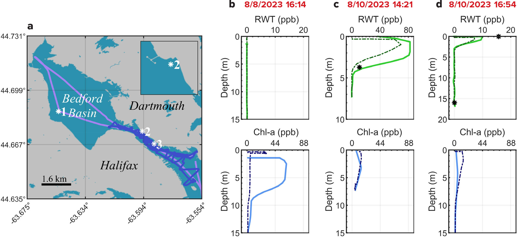
FIGURE 4. (a) GPS paths of Eastcom on August 8, 2023 (violet path) and August 10 (indigo path). Stations 1, 2, and 3 indicate locations of the vertical profiles in (b), (c), and (d), respectively. Inset: Station 2, magnified, indicates Tufts Cove Power Generation Station, the release site of the RWT. Red text in the following indicates UTC time of profile start. (b) August 8 (afternoon) pre-release profiles show zero RWT response (top) and a Chl-a profile (bottom). Solid curves indicate downcast, and dot-dashed curves indicate upcast. (c) August 10 (morning) post-release profiles stationed next to the RWT outflow; RWT channel saturates near the surface, decently agrees with Niskin bottle sample (black asterisks). (d) August 10 (afternoon) post-release profiles were made further along the anticipated path of the dye plume. Note modest underestimation of Niskin bottle RWT sample. > High res figure
|
The map provided in Figure 4a illustrates the GPS paths of the diving vessel Eastcom used for the deployment. The labeled sites indicate the profile locations: Stations 1, 2, and 3 in Figure 4b, 4c, and 4d, respectively. The bright colored curves indicate measurements while downcasting, whereas the darker dot-dashed curves indicate upcasting. The results from the Niskin bottle samples are indicated with black asterisks. The bottom-depth Niskin bottle samples were found to have no detectable RWT across the entire data set, in agreement with the PIXIE measurements.
The profiles in Figure 4b were captured on August 8, 2023, two days prior to dye release. No dye was detected while some Chl-a was detected at Station 1, the location of the DRDC (Defence Research and Development Canada) Atlantic Acoustic Calibration Barge. The vertical Chl-a profile measured by the PIXIE shows qualitative agreement with historical observations (Giesbrecht and Scrutton, 2018). The Chl-a concentration maximized by 10 m depth and returned to zero/background by 15 m depth on downcast, though the significant difference in time of day, season, and year confounds their quantitative comparison. The upcast profile appears in sharp contrast to the presented and historical downcast profiles. Because this station achieves the greatest cast depth of 45 m among the dataset, this discrepancy between downcast and upcast may indicate a pressure hysteresis effect (Shigemitsu et al., 2020) that is uncharacterized and warrants future investigation.
The profiles in Figure 4c were captured on August 10, 2023, during the RWT release at Station 2, directly in front of the Tufts Cove Power Generating Station effluent where the RWT was released. The RWT channel saturates immediately below the surface (>82.3 ppb RWT), confined to an apparent stratum between 1 m and 5 m depths. This indicates a subduction of the RWT plume that can be confirmed visually in Figure 1, but the exact mechanism of this stratification is beyond the scope of this article. The surface-depth Niskin bottle sample recorded an RWT concentration of 217.8 ppb, clearly in excess of the PIXIE’s saturation limit. A second, near-surface bottle sample (3.7 m) recorded a concentration of 10.7 ppb, in good agreement with the PIXIE’s measurement of 14.5 ppb. The discrepancy between bottle and PIXIE measurements at this depth could be attributed to the difference in interrogated volume at this point. The profile suggests that the bottle sample was taken at the edge of a steep RWT gradient. The point sampling of the PIXIE’s measurement is therefore more sensitive to depth than the ~1 m concentration gradient over which the Niskin bottle averages.
The profiles in Figure 4d were captured on August10, 2023, three hours later at Station 3, along the anticipated path of the RWT plume. The RWT channel detected a weaker but certainly present signal (10 ppb) in the first 2 m and returned to zero by 5 m depth. The surface Niskin bottle sample recorded an RWT concentration of 15.7 ppb, in modest agreement with the PIXIE’s measurement. The Chl-a channel shows a similar characteristic to that observed at the previous station, with no apparent dependence on the presence/absence of the large (>200 ppb) RWT plume.
To further validate the performance of the PIXIE, the August 10, 2023, profile at Station 3 can be compared to the nearest RWT transects captured by the ecoCTD, occurring just after the Niskin bottle samples were collected. See the online supplementary materials for a summary of the comparison of the two sets of profiles along with a waterfall plot (see Figure S2).
Conclusions
The PIXIE is a low-cost, open-source, multichannel fluorometer that demonstrates performance comparable to industry standards. It can be assembled at a cost to the end user of $741.38 USD per channel on average, and alternate configurations can be even less expensive. While this cost should not be compared to the internal cost-per-unit of industrial in situ fluorometers and the end user must consider the value of the support and quality assurance industrial devices enjoy, the PIXIE nevertheless represents an open-source option with similar performance and a low barrier to entry. The PIXIE’s limit of detection is 0.01 ppb RWT and 0.02 ppb Chl-a, which is on par with other in situ fluorometers. The PIXIE was successfully field deployed and validated as a part of a dye-tracer experiment in Halifax Harbor. The full availability of the PIXIE’s source files, from hardware to firmware, allows the end user to customize the PIXIE as much or as little as desired. The PIXIE makes a transformative leap in accessibility that can meet the growing demands for spatio-temporal data from our planet’s waterways, without sacrificing measurement quality.
Possible Future Development
A road map of future work is proposed within the PIXIE Complete User Guide available on the GitHub project page. Hysteresis has been identified (Briggs et al., 2011; Cetinić et al., 2012) as a common problem in fluorometers and similar in situ devices, and the degrees along which the PIXIE exhibits it should be studied explicitly. With some modifications to the front end, the PIXIE could include turbidity and backscattering as potential channel types along with its current fluorometric channels. Internal temperature sensing can be integrated through firmware, and external (in situ) temperature sensing could be performed in place of one of the fluorometric channels with only minor hardware changes. More details toward each of these proposed areas of future work can be found on GitHub.
Acknowledgments
We would like to thank Teo Milos, Mickey Jackson, Chidinma Onumadu, and Rehan Khalid for their senior-year project contributions in the end-cap design. We also would like to thank Iain Grundke, Edward Luy, and James Smith, from Dartmouth Ocean Technologies Inc. for advice in the early stage of the project. This work was funded in part by the Canada First Research Excellence Fund (CFREF) through the Ocean Frontier Institute (OFI) and Transforming Climate Action (TCA), the National Sciences and Engineering Research Council (NSERC) of Canada, and the Canadian Foundation for Innovation John Evans Leadership Fund. We would like to thank Ruth Musgrave, Ruby Yee, and Mathieu Dever for their contribution of fluorometry data from their transect study to this work. We further acknowledge the funding sources of their contribution; the transect study was funded in part by NSERC, the OFI, and the Trottier Family Foundation. The fieldwork in Halifax Harbor was supported in part by the Carbon to Sea Initiative, a multi-funder effort incubated by Additional Ventures, and the Thistledown Foundation. We would like to thank Claire Normandeau, Jessica Oberlander, and Lindsay Anderson for their help in analyzing RWT samples in the laboratory. We would like to acknowledge support from Douglas Wallace in providing scientific guidance and access to the infrastructure and materials at the CERC.OCEAN laboratory. The maps provided in Figure 4 and Figure S2 contain information licensed under the Open Government Licence – Canada.