Oceanography The Official Magazine of
The Oceanography Society
Volume 32 Issue 03

View Issue TOC
Volume 32, No. 3
Pages 138 - 139

OpenAccess

SIDEBAR • Submesoscale Dynamics Inferred from Oleander Data

By Jörn Callies  
Jump to
Full text Citation References Copyright & Usage
Full Text

CMV Oleander III data played a key role in advancing our understanding of submesoscale turbulence, which is suspected to control the exchange of heat, carbon, and nutrients between the surface and the interior ocean (e.g., Ferrari, 2011; Mahadevan, 2016). Insight largely came from wavenumber spectra of kinetic energy, which decompose the flow observed with the shipboard ADCP into contributions from different spatial scales that cover a range of about 10–500 km in the case of Oleander.

Ever since the seminal work of Kolmogorov (1941), Kraichnan (1967), and Charney (1971), wavenumber spectra have played a central role in turbulence theory. A key prediction of such theories is that the kinetic-energy spectrum, within an appropriately defined inertial range, falls off with wavenumber k following a power law: S(k) ~ kp. The predicted power law exponent p permits a simple comparison between theory and observations.

For the oceanic submesoscale range, two variants of turbulence theory are often discussed (e.g., Klein and Lapeyre, 2009): interior and surface quasi-geostrophic turbulence. The interior variant maps almost directly onto Kraichnan’s two-dimensional turbulence theory and predicts a power law exponent p = 3 (Charney, 1971). Such a rapid fall-off with wavenumber signifies that there is little energy at small scales—the submesoscales in this regime are comparatively benign. The presence of the sea surface changes the dynamics quite drastically because it allows for the formation of fronts and filaments and thus energetic submesoscales. The predicted power law exponent in this surface regime is p = 5/3 (Blumen, 1978). This theory, combined with idealized numerical simulations of submesoscale turbulence, led to the expectation that the submesoscales were energetic near the sea surface wherever a sufficiently strong lateral surface buoyancy gradient allowed for frontal dynamics.

The first hint that this simple conception of submesoscale dynamics was incomplete came when Wang et al. (2010) computed a wavenumber spectrum of kinetic energy along the Oleander track. They found the spectrum to fall off with an exponent of roughly p = 3 in the 20–200 km range. The spectrum is consistent with the interior prediction, despite being calculated from data within 20 m of the sea surface. This did not fit the prediction of energetic surface submesoscales that were expected in a region with strong surface buoyancy gradients, such as that between New Jersey and Bermuda.

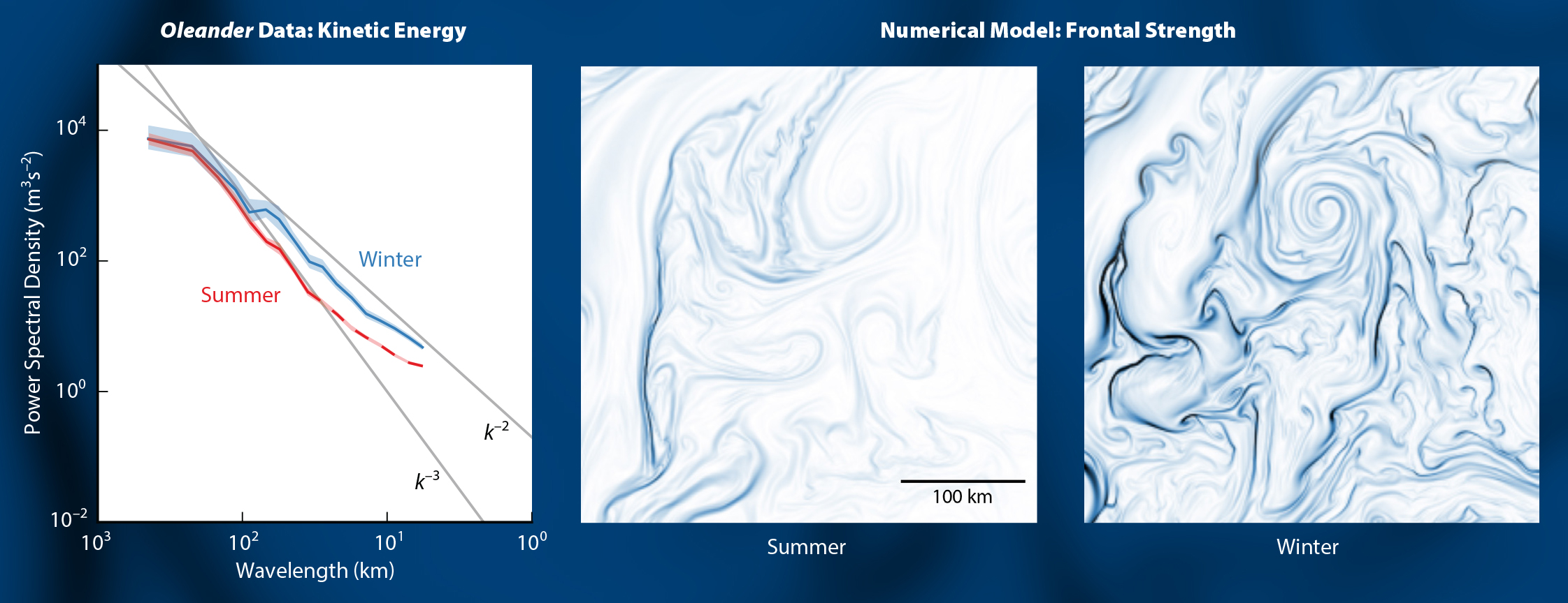
The next clue provided by Oleander data, in conjunction with data from the LatMix experiment (e.g., Shcherbina et al., 2015), was that submesoscale energy levels undergo a strong seasonal cycle (Callies et al., 2015). The steep fall-off (p = 3) is observed in the annual average only—in the winter months (January–March), submesoscale turbulence is much more energetic (p = 2, Figure 1).


Figure 1. Seasonality of submesoscale turbulence. (left) Wavenumber spectra of kinetic energy calculated from Oleander ADCP data, showing the wintertime energization of submesoscale turbulence between 10 km and 100 km. These spectra are dominated by geostrophic flow except for the small-scale end of the summer spectrum (dashed), where inertia–gravity waves dominate. (middle and right) Plan view of the frontal strength (magnitude of the surface buoyancy gradient) from a numerical model for summer (August 15) and winter (February 15). Figure adapted from Callies et al. (2015) under Creative Commons license (https://creativecommons.org/licenses/by/4.0/). > High res figure


This observation of seasonality provided a key insight. It is inconsistent with surface quasi-geostrophic turbulence, which would produce energetic submeso-
scales year-round. The seasonality is expected, however, if submesoscale turbulence is instead energized by baroclinic mixed-layer instabilities. These instabilities slide dense water under light water laterally within the mixed layer (Boccaletti et al., 2007; Fox-Kemper et al., 2008; Callies et al., 2016). They depend on the stratification contrast between the thermocline and the mixed layers, a feature of the upper ocean that in surface quasi-​geostrophic turbulence theory fell victim to idealization. Because of their dependence on the mixed layer, these instabilities are much stronger in winter, when mixed layers are deep. Oleander data helped establish these baroclinic mixed-layer instabilities as a cornerstone of our understanding of submesoscale turbulence.

But there is more that wavenumber spectra from Oleander’s ADCP data have revealed about submesoscale dynamics. It has been known for a long time that the slowly evolving meso- and submesoscale turbulence discussed so far coexists with a field of fast internal waves that permeates the ocean. It has been less clear, however, what type of motion dominates at what spatial scale. Together with data from other locations, Oleander data have revealed that the dominant dynamics transition from geostrophic turbulence at large scales to internal waves at small scales within the submesoscale range (20 km in the Oleander region; Callies and Ferrari, 2013; Bühler et al., 2014; Qiu et al., 2017). Distinguishing between these different dynamics is crucial because the irreversible stretching and folding of geostrophic turbulence is much more effective at transporting tracers than the nearly reversible wave motion.

Thus, Oleander data have helped bring into focus the dynamics that govern submesoscale ocean currents. The insight gained from the data will be crucial in determining whether and how these small-scale currents can in fact exchange heat, carbon, and nutrients between the surface and the interior ocean at rates that matter at a global level.


Citation

Callies, J. 2019. Submesoscale dynamics inferred from Oleander data. Oceanography 32(3):138–139, https://doi.org/10.5670/oceanog.2019.320.

References
    Blumen, W. 1978. Uniform potential vorticity flow: Part I. Theory of wave interactions and two-dimensional turbulence. Journal of the Atmospheric Sciences 35(5):774–783, https://doi.org/10.1175/1520-​0469(1978)035​<0774:UPVFPI>2.0.CO;2.
  1. Boccaletti, G., R. Ferrari, and B. Fox-Kemper. 2007. Mixed layer instabilities and restratification. Journal of Physical Oceanography 37(9):2,228–2,250, https://doi.org/10.1175/JPO3101.1.
  2. Bühler, O., J. Callies, and R. Ferrari. 2014. Wave-vortex decomposition of one-dimensional ship-track data. Journal of Fluid Mechanics 756:1,007–1,026, https://doi.org/10.1017/jfm.2014.488.
  3. Callies, J., and R. Ferrari. 2013. Interpreting energy and tracer spectra of upper-ocean turbulence in the submesoscale range (1–200 km). Journal of Physical Oceanography 43(11):2,456–2,474, https://doi.org/10.1175/JPO-D-13-063.1.
  4. Callies, J., R. Ferrari, J.M. Klymak, and J. Gula. 2015. Seasonality in submesoscale turbulence. Nature Communications 6:6862, https://doi.org/10.1038/ncomms7862.
  5. Callies, J., G. Flierl, R. Ferrari, and B. Fox-Kemper. 2016. The role of mixed-layer instabilities in submesoscale turbulence. Journal of Fluid Mechanics 788:5–41, https://doi.org/10.1017/jfm.2015.700.
  6. Charney, J.G. 1971. Geostrophic turbulence. Journal of the Atmospheric Sciences 28(6):1,087–1,095, https://doi.org/​10.1175/​1520-0469(1971)028​<1087:GT>2.0.CO;2.
  7. Ferrari, R. 2011. A frontal challenge for climate models. Science 332(6027):316–317, https://doi.org/​10.1126/science.1203632.
  8. Fox-Kemper, B., R. Ferrari, and R.W. Hallberg. 2008. Parameterization of mixed layer eddies; Part I. Theory and diagnosis. Journal of Physical Oceanography 38(6):1,145–1,165, https://doi.org/​10.1175/2007JPO3792.1.
  9. Klein, P., and G. Lapeyre.2009. The oceanic vertical pump induced by mesoscale and submesoscale turbulence. Annual Review of Marine Science 1:351–375, https://doi.org/10.1146/annurev.marine.010908.163704.
  10. Kolmogorov, A.N. 1941. The local structure of turbulence in incompressible viscous fluid for very large Reynolds numbers. In Russian: Doklady Akademii Nauk SSSR 30:301–305. Translated into English: Proceedings of the Royal Society A 434(1890):9–13, https://doi.org/10.1098/rspa.1991.0075.
  11. Kraichnan, R.H. 1967. Inertial ranges in two-​dimensional turbulence. Physics of Fluids 10(7):1,417–1,423, https://doi.org/​10.1063/1.1762301.
  12. Mahadevan, A. 2016. The impact of submesoscale physics on primary productivity of plankton. Annual Review of Marine Science 8(1):161–184, https://doi.org/​10.1146/​annurev-​marine-​010814-​015912.
  13. Qiu, B., T. Nakano, S. Chen, and P. Klein. 2017. Submesoscale transition from geostrophic flows to internal waves in the northwestern Pacific upper ocean. Nature Communications 8(14055):1–10, https://doi.org/10.1038/ncomms14055.
  14. Shcherbina, A.Y., M.A. Sundemeyer, E. Kunze, E. D’Asaro, G. Badin, D. Birch, A.-M.E.G. Brunner-Suzuki, J. Callies, B.T. Keubel Cervantes, M. Ciaret, and others. 2015. The LatMix summer campaign: Submesoscale stirring in the upper ocean. Bulletin of the American Meteorological Society 96(8):1,257–1,279, https://doi.org/10.1175/BAMS-D-14-00015.1.
  15. Wang, D.-P., C.N. Flagg, K. Donohue, and H.T. Rossby. 2010. Wavenumber spectrum in the Gulf Stream from shipboard ADCP observations and comparison with altimetry measurements. Journal of Physical Oceanography 40(4):840–844, https://doi.org/10.1175/2009JPO4330.1.
Copyright & Usage

This is an open access article made available under the terms of the Creative Commons Attribution 4.0 International License (https://creativecommons.org/licenses/by/4.0/), which permits use, sharing, adaptation, distribution, and reproduction in any medium or format as long as users cite the materials appropriately, provide a link to the Creative Commons license, and indicate the changes that were made to the original content. Images, animations, videos, or other third-party material used in articles are included in the Creative Commons license unless indicated otherwise in a credit line to the material. If the material is not included in the article’s Creative Commons license, users will need to obtain permission directly from the license holder to reproduce the material.