Since late fall 1992, CMV Oleander III has been measuring upper ocean currents during its weekly trips between Bermuda and Port Elizabeth, New Jersey, by means of an acoustic Doppler current profiler installed in its hull. The overarching objective of this effort has been to monitor transport in the Gulf Stream and surrounding waters. With 25 years of observation in hand, we note that the Gulf Stream exhibits significant year-to-year variations but no evident long-term trend in transport. We show how these data have enabled studies of oceanic variability over a very wide range of scales, from a few kilometers to the full 1,000 km length of its route. We report that the large interannual variations in temperature on the continental shelf are negatively correlated with flow from the Labrador Sea, but that variability in the strength of this flow cannot account for a longer-term warming trend observed on the shelf. Acoustic backscatter data offer a rich trove of information on biomass activities over a wide range of spatial and temporal scales. A peek at the future illustrates how the new and newly equipped Oleander will be able to profile currents to greater depths and thereby contribute to monitoring the strength of the meridional overturning circulation.

 

> High res

Introduction

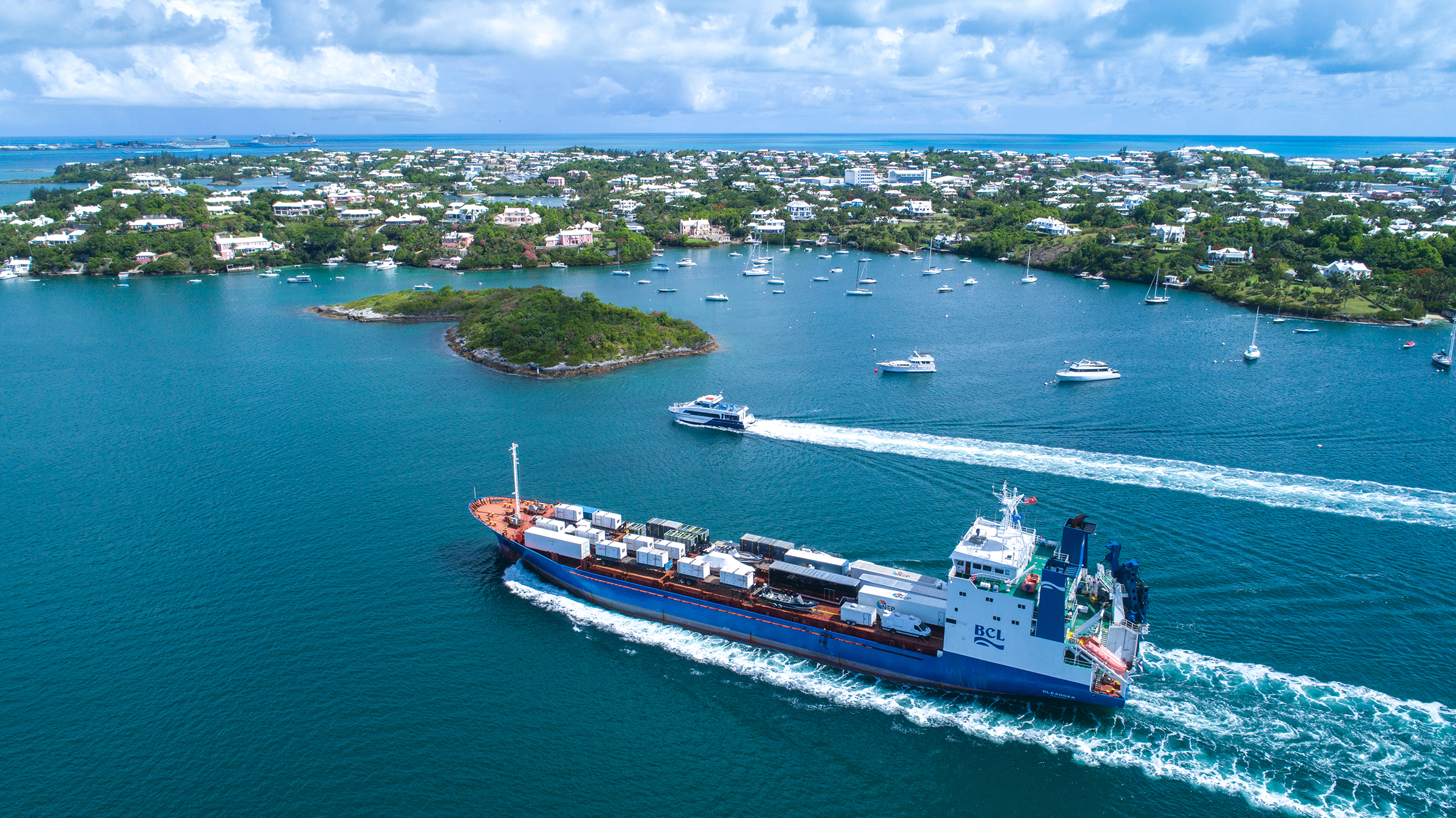
More than a flower indeed, the name Oleander refers to the container vessel CMV Oleander III that operates on a weekly schedule between Bermuda and Port Elizabeth, New Jersey. With an instrument in its hull to measure upper ocean currents, the ship crosses four major water masses of the North Atlantic: subtropical water in the Sargasso Sea, warm salty water carried from the tropics in the Gulf Stream, cold fresh waters from the Labrador Sea in the Slope Sea, and the waters on the continental shelf. What makes this line so special is not only that such diverse water masses occur in close proximity to one another but also that Oleander crosses them all twice a week. Starting in fall 1992 when we installed an acoustic Doppler current profiler (ADCP) in the hull of Oleander, we have been monitoring upper ocean currents along the ship’s transits between Bermuda and New Jersey.

The primary objective of the Oleander program has been and continues to be to monitor the strength of the Gulf Stream: how does it vary by season and from year-to-year, and do these variations show any patterns that might be suggestive of longer-​term trends? The same questions can of course be asked of the surrounding waters. We have also been profiling temperature to ~900 m depth along the route with eXpendable BathyThermographs (XBTs), extending a long-running XBT program maintained by NOAA. In this article, we provide an up-to-date summary of what we have learned from these activities since the start of the program a little over 25 years ago. Figure 1 shows the Oleander route in relation to the Gulf Stream, with the Slope Sea and continental shelf to its north and the Sargasso Sea to its south. The flow in the Gulf Stream here is to the east, while everywhere else across the Oleander route it is on average to the west.

 

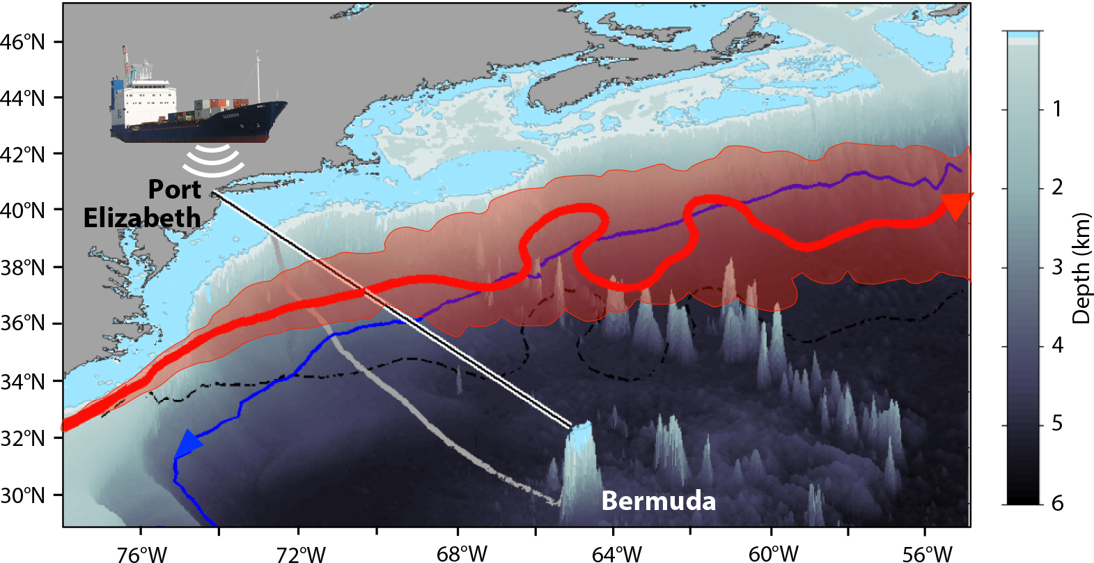
Figure 1. Oleander transect between Port Elizabeth, New Jersey, and Hamilton, Bermuda (black line, with its “shadow” on the seafloor in gray. The pink shaded region represents the Gulf Stream meander envelope based on the monthly mean Gulf Stream paths from the 25 cm sea surface height contour in mapped satellite altimetry from 1993 through 2014. The red line is a representative Gulf Stream path from one of these monthly means (with its dashed black “shadow” on the seafloor). The solid blue line is the 4,000 m isobath along the slope, where the Deep Western Boundary Current is flowing in the direction opposite to that of the Gulf Stream. The region shallower than 100 m depth is shaded blue. > High res figure

 

We begin with a review of the principal findings of our Gulf Stream studies, the main focus of the Oleander program. As we do so, we will point to other, more technical, papers that address some issues in further detail. A neat aspect of the Oleander project is how it has supported or enabled a number of diverse research activities in addition to the Gulf Stream studies. One question of great interest to which it has contributed concerns transport variability on the continental shelf and slope. Similarly, the sustained sampling has enabled detailed statistical studies of coherent vortices, the formation of rings from extended meanders, and “stroboscopic” studies of cold core rings after they have been formed. The ADCP also provides fascinating information on the backscatterers, principally large zooplankton and small fish, in the water column. All of this science has come from a single instrument in continuous operation except while in port. The new CMV Oleander, which began service in April 2019, is equipped with a 150 kHz and a 38 kHz ADCP. We can take a peek at what to expect from this ship using similar 38 kHz ADCP data from Explorer of the Seas, which has on occasion operated along the same route from New Jersey to Bermuda. We use these data to demonstrate how the new vessel will be able to contribute to the monitoring of the strength of the meridional overturning circulation (MOC) and concomitant heat and freshwater fluxes.

 

The ADCP

The key tool of the Oleander program has been the ADCP, an instrument that measures currents relative to the ship from below the vessel to a maximum depth that depends in part upon the operating frequency of the ADCP (Flagg et al., 1998). Between late 1992 and 2004, we operated a 150 kHz ADCP that reached to roughly 250–300 m in the Slope Sea, 400 m in the Gulf Stream, and 250 m in the Sargasso Sea. It was replaced in 2005 with a 75 kHz instrument that remained in operation until summer 2018. It could reach below 600 m everywhere. The measurements start at 20–40 m depth, depending upon instrument type. How deep a profile reaches also depends on density of backscatterers (primarily zooplankton and myctophids) and weather conditions. In heavy weather, air bubbles swept underneath the hull can quite effectively block the ADCP acoustics. In general, data returns are better on Bermuda-bound transits because the vessel is more heavily loaded and because it tends to have following winds when southbound. Weather can improve or get worse during a transit, so the data return can be quite variable. This variable data return from transit-to-transit is the main reason we do not attempt to look at timescales faster than seasonal. The ADCP signal can be also viewed like an acoustic X-ray, where intensity depends upon the biomass present. However, the backscatter strength is not a quantitative measure of biomass because we do not know its composition. But as we will see later, it can be very informative about the dynamics of the backscatterers.

What makes measuring currents from a fast-moving vessel possible is the GPS-based compass, which enables us to measure the ship’s speed and heading with such precision that we can determine currents over the bottom to ±0.01 m s^–1 accuracy (Flagg et al., 1998). The left panels in Figure 2 show a high-quality section of temperature (XBTs), and zonal and meridional velocity along the Oleander route. Note how the temperature surfaces deepen by about 600 m from north to south across the narrow rapid current. This ~600 m dip is in fact almost the same at all depths (see Fuglister, 1963; Halkin and Rossby, 1985). The tight co-location between the sharp change in temperature and maximum velocity reflects the well-established thermal wind relationship between velocity and density (temperature): vertical shear is balanced by the horizontal density gradient, ∂v/∂z = –g/(ρf) ∂ρ/∂x, where g, ρ, and f represent gravity, density, and the Coriolis parameter, respectively.

 

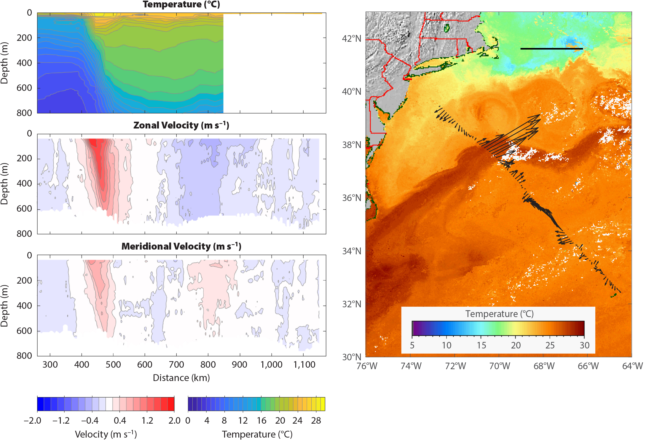
Figure 2. A concurrent eXpendable BathyThermograph (XBT) and acoustic Doppler current profiler (ADCP) section across the Gulf Stream July 4–6, 2009. The sampling density is about 20 km for temperature and 2.2 km for velocity. The right panel shows a three-day composite (July 3–5) sea surface temperature at the time of the transit (courtesy of the Applied Physics Laboratory of Johns Hopkins University). Vectors are ~11 km apart, maximum velocity vector = 1.96 m s–1 (bar at top ~2 m s–1). Distances are shown from New York City. > High res figure

 

In addition to measuring currents directly, this figure highlights another advantage of the ADCP—it provides far higher spatial resolution than is possible with XBTs. The right panel shows a three-day composite (to remove presence of clouds) of sea surface temperature at that time with the near-surface velocity vectors superimposed.

A major strength of the vessel-mounted ADCP lies in its ability to accurately scan and profile (~0.01 m s^–1) the horizontal structure of the velocity field over a wide range of scales, from a few kilometers to the full length of the section. We will use the verb “scan” hereafter to emphasize this particular skill of ships in transit: to cost-effectively and accurately measure (“X-ray,” if you will) ocean currents. There is a certain irony in this. For more than a century, oceanographers have used hydrography to estimate currents and transports. This changed in the 1970s with the advent of moored current meters and neutrally buoyant floats that provided a far better measure of the temporal and spatial characteristics of ocean currents. These efforts have been extremely productive (Robinson, 1983), and they continue today. Here, we show how ships in regular traffic can extend those moored capabilities. The irony here is that a single instrument on a ship in regular traffic can repeatedly scan ocean currents and thus resolve long-term variability of currents and transports far more accurately and at lower cost than is possible with hydrography or moored resources. This is not a trivial point. Today, we have come to recognize that accurate estimates of transport of mass, heat, and freshwater, all of great importance to the ocean’s role in climate, depend primarily upon knowing the velocity field. We know the temperature and salinity fields well enough that further improvement in estimating mass, heat, and freshwater fluxes will depend critically upon how well we can determine the velocity field. This is where ships in regular and repeat service can be invaluable (SCOR/IAPSO Working Group 133, 2012).

 

AXIS

AXIS (for Autonomous eXpendable Instrument System) has been a major enhancement to the Oleander operation. For years, NOAA, through its Ship Of Opportunity Program (SOOP), sent an observer along to launch XBTs to obtain vertical sections of temperature across the continental shelf out to the Gulf Stream. To improve coverage along the entire route, AXIS was developed. It normally functions completely autonomously under a preset schedule, but it can be contacted at any time to deploy XBTs into features of interest along the vessel’s route (Fratantoni et al., 2017). For example, if a warm- or cold-core ring is passing by, a shore-based observer can schedule probes to be dropped in rapid succession. All that is required of the ship is that a member of the crew reloads AXIS as needed. With AXIS, we can now deploy XBTs, or probes of all approved types including XCTDs, at any time and anywhere along the route to Bermuda. With the continued generous support of the NOAA SOOP, XBT sections are taken monthly on the Oleander route, and the data, relayed by Iridium, are available to the user community and the public at large within 24 hours.

 

Basic Findings

The repeat and sustained sampling of the velocity field by Oleander gives us the framework for studies of long-term transport variability in the ocean. The left panel of Figure 3 shows the mean velocity vectors and variance ellipses at 52 m depth along the route, the result of over 1,000 highly resolved scans of velocity between late 1992 and mid 2018. These vectors and variance ellipses can be viewed as coming from a virtual array of ~300 moorings 3 km apart with current meters densely spaced in the vertical. This analogy applies, of course, only to frequencies well below the sampling rate, which at best would be twice per week. In practice, the fastest timescales we attempt to quantify are seasonal variations (Rossby et al., 2010). It is worth noting that only the Gulf Stream flows northeast between the continent and Bermuda. In fact, the Gulf Stream is effectively the only poleward flowing current in the entire North Atlantic; everywhere else, ocean currents flow or trend to the south, both at the surface and at depth. We will return to this later. The strong westward flows to either side of the Gulf Stream are recirculation gyres driven by the meandering Gulf Stream. The northern recirculation gyre as well as water on the shelf includes a significant contribution of water from the Labrador Sea. In between the shelf and the Slope Sea the westward flow exhibits a well-defined minimum, perhaps a result of greater dynamic drag by the sloping bottom? The meandering Gulf Stream drives a substantial anti-
cyclonic recirculation to its south. The variance ellipses are large, but conspicuously localized to the Gulf Stream. A close look will show that the ellipses to either side “toe in” (i.e., point toward the center of the current). This may reflect the fact that the meander envelope is tightening in this area as indicated by sea surface height variability (Starr, 1968; Rossby, 1987). That the Oleander route crosses the Gulf Stream so close to a meander minimum has undoubtedly made it easier to monitor transport variations more accurately.

 

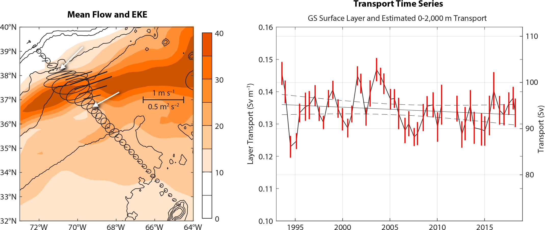
Figure 3. (left) Mean velocity and variance ellipses from the continental shelf edge to Bermuda for the entire observing period, 1992–2018. Horizontal bar = 1 m s–1 and 0.5 m2s–2. The color field indicates the standard deviation of the sea surface height (unit: cm) for the same 1992–2018 period. Bathymetric contours at 200, 1,000, 2,000, 3,000, and 4,000 m depth. The white arrows delineate th edge of the Gulf Stream. EKE = eddy kinetic energy. (right) Annually averaged Gulf Stream (GS) layer transport (at 52 m depth) for the entire record in half-year steps. The red bars indicate the standard deviation for that period. Solid and dashed lines represent a linear fit and 95% confidence limits. The right axis shows the 0–2,000 m transport, assuming a scale factor of 700 (see text). > High res figure

 

The right panel of Figure 3 shows the temporal variations in layer transport (i.e., transport in a 1 m thick layer centered at 52 m depth) since the start of the program. It is an update of a figure first published by Rossby et al. (2014). The definition of Gulf Stream transport is specific. It is the downstream velocity component parallel to its maximum integrated from one side to the other with the edges defined by where the velocities first change sign near the surface. This accords with the classical hydrographic definition, where the current is delineated by the maximum dynamic height difference across the current. The right y-axis shows estimated transport between the surface and 2,000 m depth using a scale factor 700 (Rossby et al., 2014) with an average ~94 Sv (1 Sverdrup = 10⁶ m³ s^–1). The interannual variations in transport appear to be quite large, but are only about 4%–5% of the mean for timescales of a year or longer. Significantly, the plot shows no evident long-term trend over the 25-year record. While the Gulf Stream transport includes far more transport than the 16–18 Sv MOC transport (e.g., Sarafanov et al., 2012; McCarthy et al., 2015), any trend over the last 25 years is only about 1–2 Sv, and maybe less, given the 95% uncertainty limits in the panel. Unless there is some kind of conspiracy between MOC and wind-driven change in transport so they cancel, this suggests that the MOC is stable at the 1 Sv level on these timescales. This is not to say that it may not slow down or increase more markedly in the future, but it does not lend support to suggestions that the MOC already has started slowing down substantially (see Sallenger et al., 2012; Ezer et al., 2013). The lack of evidence for a Gulf Stream slowdown accords with an earlier study that found the baroclinic transport varied widely, but no signal of decline emerged from this variability between the 1930s and 1980s (Sato and Rossby, 1995; also, using reanalyzed data from the 1873 Challenger Expedition, Rossby et al., 2010, found that geostrophic transport by the Gulf Stream at that time fell in line with the Sato and Rossby study).

The method of estimating transport by integrating to the velocities’ first zero crossing to either side of the Gulf Stream does not lend itself to comparison with satellite estimates of geo­strophic flow based on sea surface height (SSH) field because the latter do not have the necessary spatial resolution to accurately resolve the edges of the meandering stream. But it is still of great importance to establish how well altimetry agrees with direct measurement of currents—a comparison that relies on the fact that motions on scales >O(10) km are substantially geostrophic. Worst et al. (2014) tested this by defining fixed points to either side of the Gulf Stream where SSH exhibits a variance minimum between which SSH difference across the stream can be determined. They find high correlations (>0.9) provided altimetry measurements are interpolated to the same day as the ADCP transect. This result is of great value, for it means that the ADCP velocities are not only accurate but also unbiased, affirming that measuring currents and transports from fast-moving vessels is quite feasible. But insofar as the Gulf Stream alone is concerned, the ADCP with its excellent and accurate spatial resolution does a far better job of estimating Gulf Stream transport because, as noted, it can accurately determine the limits of integration.

 

The Gulf Stream in Natural or Stream Coordinates

Each Oleander transit gives us a snapshot or synoptic view of the velocity field in the Gulf Stream. The ensemble of these can be used to construct the dense array of Eulerian mean velocities and variance ellipses as shown in Figure 3. But we have long known that the Gulf Stream, viewed locally, is a rather narrow, swift current. Whether in terms of temperature (the classic view) or velocity (as here), you know when you are in it. This begs the question of how well defined it actually is, or how stiff it is, a question first addressed by Halkin and Rossby (1985). We can take the same approach here. Specifically, we transform all ADCP data into a coordinate system defined by the location and direction of the maximum velocity vector, as in Figure 4. The top panels show mean downstream and cross-stream velocity. Having aligned the velocity vectors, we obtain a maximum speed of 2.13 ± 0.29 m s^–1. The velocity structure exhibits conspicuous asymmetry, with the width of the northern or cyclonic side of the stream much thinner than the southern side. The top right shows average velocity normal to the stream. It is very weak everywhere, with a slight flow south (out of the current). The lower panels show the corresponding variances 2> and 2>. The bright band on the left side of the velocity maximum indicates that the northern shear zone is where most of the structural variability is found. That the variance in the cross-stream velocity is weak and increases only gradually from the center suggests considerable cross-stream stiffness. Velocity variance is greater on the Sargasso Sea side than in the Slope Sea; this can be anticipated from the variances ellipses in Figure 3 (left panel). It is instructive to compare eddy kinetic energy (EKE) in geographical and stream coordinates. Averaging EKE from 55 m to 600 m depth and 100 km to either side of the velocity maximum gives the average EKE = 0.26 m² s^–2 in geographical coordinates, whereas in stream coordinates it is 0.03 m² s^–2, nearly a factor 10 less. The near 90% reduction in EKE reflects the removal of the effect of Eulerian sampling of a relatively stiff (but meandering) current.

 

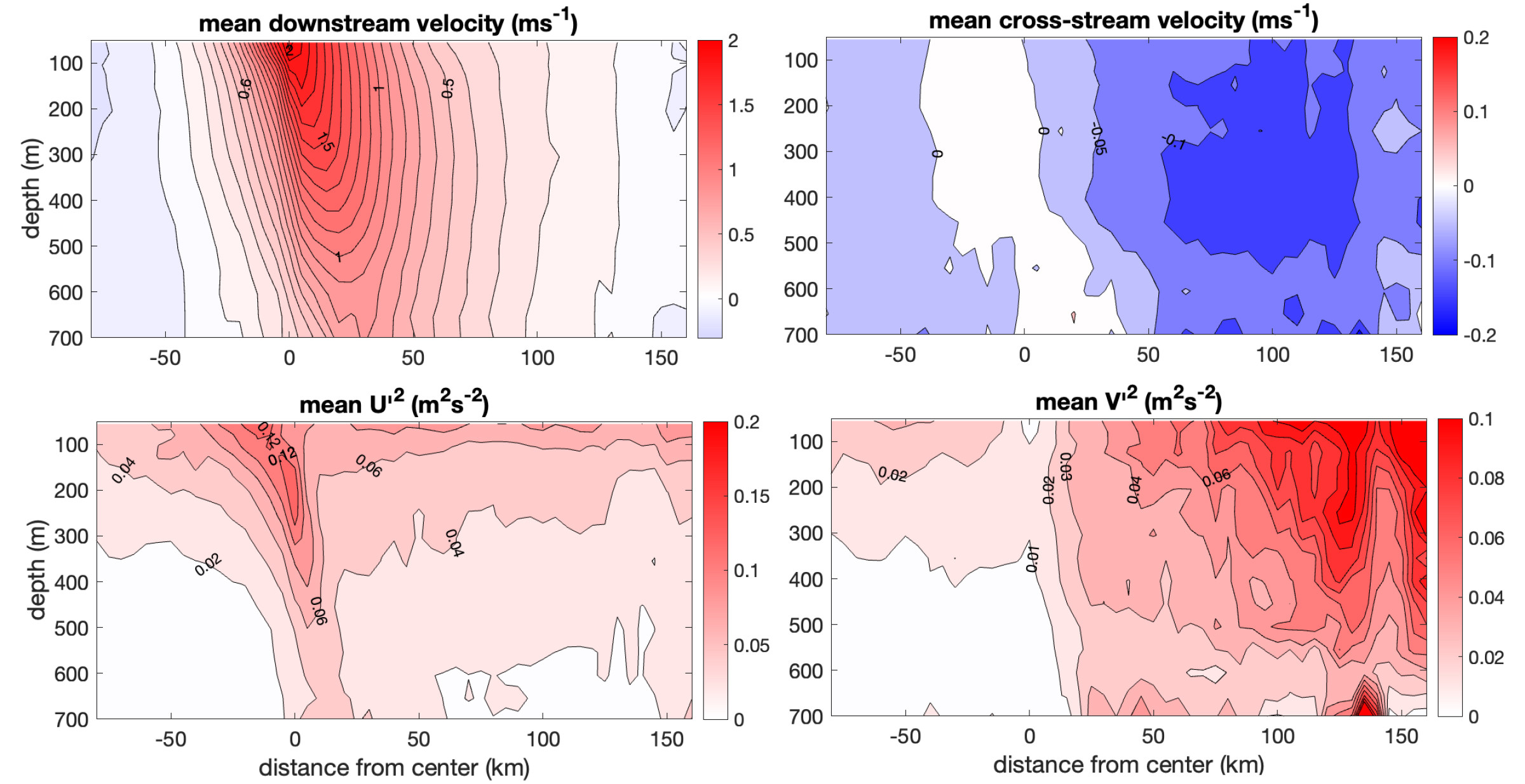
Figure 4. The Gulf Stream in stream or natural coordinates, based over 250 transects made between 2005 and 2018. The top row shows mean velocity in downstream and cross-stream directions (positive into and to left) in m s–1. The bottom row shows corresponding variance patterns in m2s–2. Note the different scales to the right of each panel. > High res figure

 

A Gallery of Studies

Here, we give a brief potpourri of the many studies to which the Oleander data have contributed.

• Oceanographers have used remote sea surface temperature imagery, specifically the sharp temperature drop at what is referred to as the North Wall to determine the location of the Gulf Stream. Here, the combination of velocity and ADCP-measured temperature gives us a coherent data set with which to determine relationships between the velocity maximum (the core of the current), the thermal North Wall (maximum temperature drop), and maximum temperature (see Figure 5). The North Wall is close, only about 20 km north of the velocity maximum. Similarly, the maximum temperature lies roughly 20 km to the south thereof, but both exhibit considerable scatter.

 

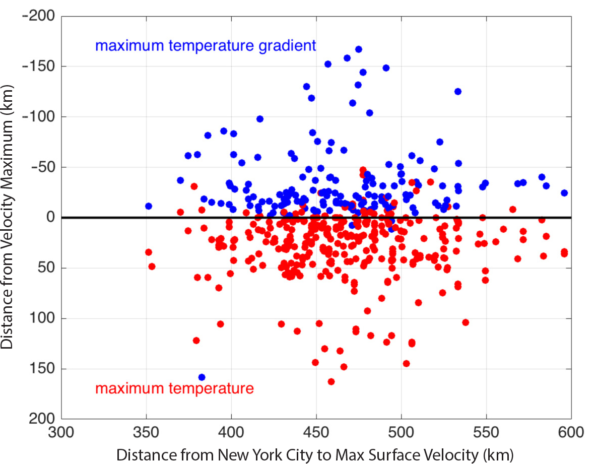
Figure 5. The blue dots show the position of a thermal north wall defined by the largest temperature drop to the north in the section relative to maximum velocity of the Gulf Stream. The red dots indicate the warmest temperature relative to the maximum velocity. The x-axis shows the position of velocity maximum along the Oleander line, and the y-axis shows distance from maximum velocity. > High res figure

 

• The Oleander data set has provided Gulf Stream metrics anchored by in situ observations that have been used evaluate the fidelity of ocean models and reanalysis products (e.g., Chassignet and Xu, 2017; Chi et al., 2018).
   
• With a goal toward improving forecasts of Mid-Atlantic Bight circulation, Levin et al. (2018) produced an improved mean dynamic topography product for the Mid-Atlantic Bight. Oleander observations provided the critical mean velocity observations in the slope region used to constrain their climatological assimilation model.
   
• Oleander data have been used to estimate wavenumber spectra from the ADCP measurements (Wang et al., 2010). Please see Callies (2019, in this issue).
   
• Rossby and Zhang (2001) used the combination of ADCP velocity and XBT temperature to examine the mean potential vorticity structure of the Gulf Stream. They found that layer thickness variations to either side of the velocity maximum compensate for lateral shear (or shear vorticity) such that the potential vorticity to either side remained nearly constant. The jump in potential vorticity from one side to the other was compressed to a very narrow zone, about one-tenth the width of the current, centered at the velocity maximum. The scale width of the two sides matches almost perfectly with the corresponding radius of deformation.
   
• A vessel in rapid transit sees the ocean “frozen in time.” Taking advantage of this, Luce and Rossby (2008) developed an algorithm for coherent vortex detection from the rotation of the velocity vector during the vessel’s transit through it. They found near equipartition of cyclonic and anticyclonic coherent vortices in the Sargasso Sea. Figure 6 shows the meander pinch-off and spin-up of a cold-core ring over a two-week period. We have experimented with extending this technique to sample cold core rings of varying age (i.e., in a form of “stroboscopic” sampling).

 

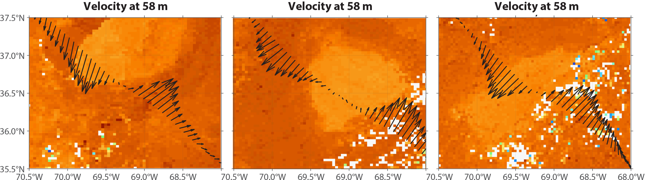
Figure 6. Three panels, a week apart between September 2 and September 16, 2000, show the velocity field during the pinch-off of a cold-core ring. The vectors are superimposed on a zoom-in of sea surface temperature. In the left panel, the cooler water (lighter colors) has not broken off from the Gulf Stream (farther north, not shown; see Luce and Rossby, 2008), whereas in the other two images, one and two weeks later, the ring has separated from the Gulf Stream. The vectors in the middle image indicate slack water in the center whereas in the last image the ring appears to have achieved solid body rotation. The color scale is the same as in Figure 2 (right panel). Maximum velocities ~2 m s–1. > High res figure

 

• The ADCP measures the strength of the backscattered signal it uses to measure the velocity-induced Doppler shift. This signal strength contains much information about spatial and temporal behavioral patterns of zooplankton and small nekton. Please see Palter et al. (2019, in this issue).
   
• Addressing a question many had asked, Sanchez-Franks et al. (2014) were unable to find any connection or correlation between transport variations at the Oleander line and the Florida Straits.
   
• Flagg et al. (2006) identified a narrow west-flowing current in the top 300 m of the Slope Sea transporting about 2.5 Sv (see next section).
   
• Stoermer (2002) demonstrated that it is possible to extract the Ekman spiral in the ADCP data from a fast-​moving vessel. However, because the Ekman velocities and scales depend so strongly upon local conditions, it proved necessary to scale velocity and depth into non-dimensional form prior to averaging.

 

Interannual-to-Decadal Variability on the Middle Atlantic Bight Shelf and Upper Slope

Whereas the Oleander data show the Gulf Stream transport to vary interannually but with little trend, recent studies have pointed to the US eastern seaboard north of Cape Hatteras as a region of dramatic change that manifests itself in sea level (Sallenger et al., 2012; Andres et al., 2013), ocean temperature (e.g., Mills et al., 2013; Pershing et al., 2015), and oxygen (Gilbert et al., 2005; Claret et al., 2018). Observed changes in coastal, shelf, and upper-slope waters here reflect not only slow processes that cause long-term ocean warming or sea level rise but also higher frequency processes that result in strong interannual variability. These trends and year-to-year changes have important ecological, economic, and social impacts. Because of their quality, continuity, and long duration, the Oleander ADCP and XBT data sets are uniquely suited both for characterizing changes on the Middle Atlantic Bight (MAB) shelf and upper slope and for investigating underlying processes that drive interannual to decadal variability.

Over the last 40 years of XBT sampling from Oleander, the annually and vertically averaged temperature across the MAB shelf has increased by about 1.25°C. This warming on the MAB shelf is superimposed on strong interannual variability (Figure 7, inserts). The warming trend over the last 15 years is not distributed uniformly across the shelf nor is it concentrated near the surface, as might be expected if it were driven primarily by local atmospheric heating. Rather, it is strongest at the shelf break (see Figure 8c in Forsyth et al., 2015). Likewise, the interannual variability in the MAB shelf temperatures is also concentrated at the shelf break (see Figure 9 in Forsyth et al., 2015).

The Oleander data have helped us to identify a connection between temperature and the strength of the Shelfbreak Jet, a 20 km wide equatorward-flowing surface current that is part of a system of currents along the shelf break stretching from the Labrador Sea to Cape Hatteras (Linder and Gawarkiewicz, 1998; Fratantoni and Pickart, 2007). Using the data from Oleander’s 75 kHz ADCP to generate a mean velocity section, the Shelfbreak Jet is evident as an along-shelf flow reaching 8 cm s^–1 (black contours in Figure 7, both panels) in waters of approximately 100 m depth. Offshore of this, and separated by a velocity minimum, another equatorward current, the Slope Jet (Flagg et al., 2006) reaches 10 cm s^–1. Conditionally averaging the velocity sections according to the annually averaged temperature on the shelf suggests that a warmer MAB shelf is in part caused by less cool water being advected along the shelf from the east (Figure 7, top panel). In colder years, an intensified shelf break jet can transport more cooler water to the MAB, and thus lead to a colder than average year in the MAB (Figure 7, bottom panel). But no evidence has been found that this velocity-temperature correlation extends to the longer-term warming trend—a question of considerable interest to many as noted earlier.

 

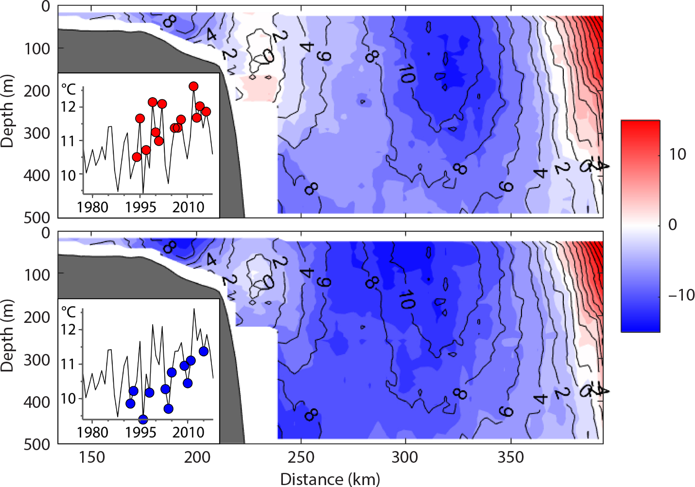
Figure 7. The two panels show velocity parallel to the shelf break across the shelf into the Slope Sea during anomalously warm and cold years. The contours in both show the overall mean velocity based on 580 ADCP crossings. The top panel shading shows the velocity when the shelf is anomalously warm (338 ADCP/56 XBT sections), and the shading in the bottom panel depicts velocity measured in years when temperatures were anomalously cold on the shelf (242 ADCP/50 XBT sections), with temperatures averaged annually and spatially across the 160 km wide shelf inshore of the 100 m isobath (see insert, based on Forsyth et al., 2015, updated here through 2017). > High res figure

 

A Peek at the Future

During the years 2006–2010, the cruise vessel Explorer of the Seas occasionally operated along the same route as CMV Oleander III. The ship was equipped with 38 kHz and 150 kHz ADCPs, the same complement as on the new Oleander. With 57 sections from primarily the 2007–2008 period, we can construct the mean Eulerian velocity field normal to the ship track between Bermuda and New Jersey for the top 1,250 m and thus get an idea of what the 38 kHz ADCP on the new vessel will be able to deliver (Figure 8, top left panel). With a 1,200+ m reach (roughly twice the capability of the 75 kHz), the ship can scan currents from the surface to below the center of the main thermocline where maximum stratification (on the 12°C isotherm) occurs at ~800 m just south of the Gulf Stream. The average peak velocity in the Gulf Stream ranges from about 1.1 m s^–1 at the surface to 0.1 m s^–1 at 1,200 m depth, numbers quite similar to those of Halkin and Rossby (1985). The flow outside the Gulf Stream is everywhere weakly to the southwest except between 700 km and 780 km due to the occasional presence of cyclonic cold core rings passing west through the section in this data set.

 

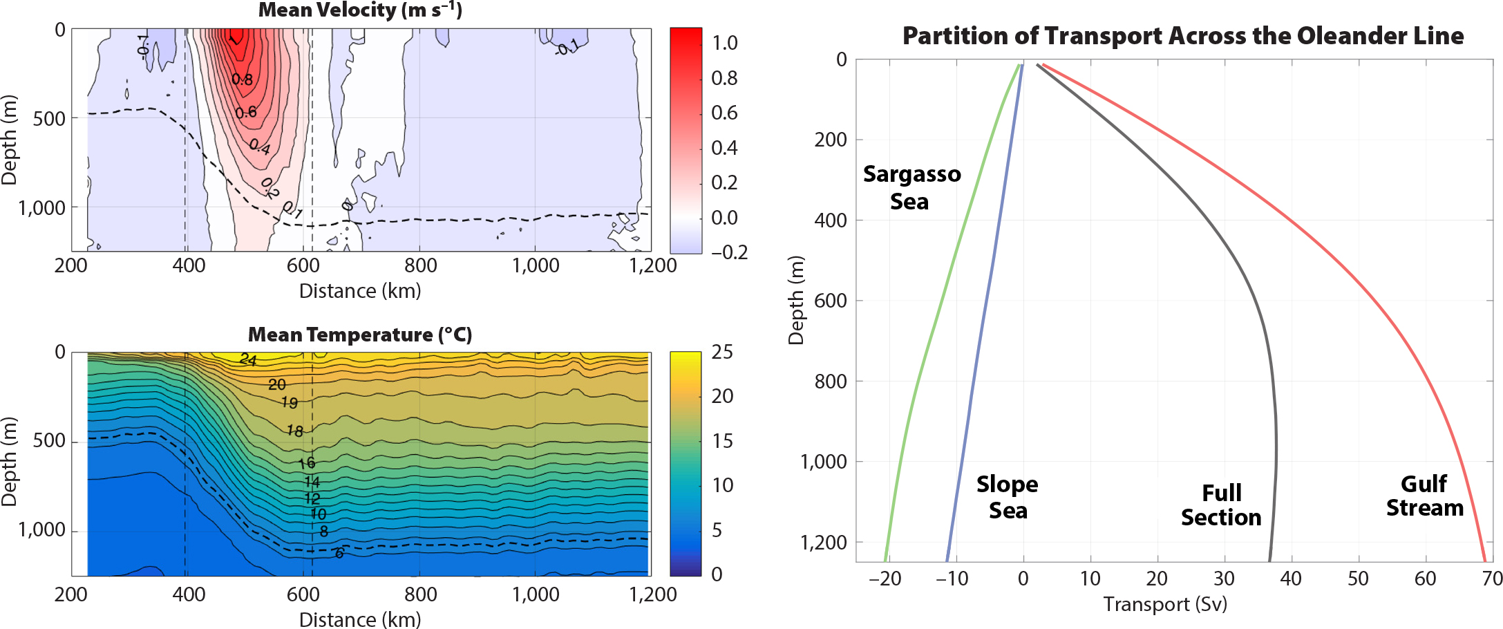
Figure 8. (top left) Mean velocity perpendicular to the Oleander route based on 57 ADCP sections primarily from 2007 and 2008 (with the rest from 2006 and 2010). (bottom left) Mean temperature from 73 XBT sections taken from 2011 to 2018. The dashed contour highlights the 6.5°C isotherm (~27.55 kg m–3 density surface). The vertical dashed lines in the left panels delineate the Gulf Stream from waters of the Slope and Sargasso Seas (white arrow points in Figure 3). (right) Integrals of transport from the surface down for the Slope Sea (blue), the Gulf Stream (red), and the Sargasso Sea (green), and the sum of all three (black). > High res figure

 

The vertical integral of velocity across the entire section from the surface down is instructive. It increases rapidly near the surface, but slows gradually, and decreases slowly after passing through a broad 38 Sv peak near 950 m depth (black curve, right panel in Figure 8). This reflects the baroclinic or strongly sheared contribution of the Gulf Stream (red line) being overtaken by the near depth-​independent flows in the Slope and Sargasso Seas (blue and green lines). Interestingly, the 950 m depth of the transport maximum lies close to what most studies suggest as the depth of the stream function maximum of the MOC (e.g., McCarthy et al., 2015). Perhaps this is not so surprising because northward flow of the upper limb of the MOC resides entirely inside the Gulf Stream; there is no other poleward flow in the North Atlantic. This means that whatever its magnitude, it is embedded within the Gulf Stream portion of the 38 Sv transport maximum. If we assume that the continental-slope-to-Bermuda integral of the Oleander section fully captures the contributions of the northern and southern recirculation gyres (the westward flows to either side of the Gulf Stream) such that these cancel out, then the horizontal, wind-driven Sverdrup circulation must make up the difference. The Sverdrup gyre occupies, indeed defines, the subtropical circulation between North Africa and North America. There are various means for estimating its strength. Here, we postulate that if there is no layer transport at 950 m for the Oleander line, then the same should be true between Bermuda and North Africa. The dynamic height difference (not shown) between the latter yields a southward transport of ~20 Sv from the surface to 900–1,000 m depth. This transport must flow north between New Jersey and Bermuda. Talley et al. (2011, Chapter 9) report a similar amount. Subtracting 20 Sv from the measured 38 Sv leaves 18 Sv, which we interpret as the strength of the upper limb of the MOC; this agrees well with other estimates (McCarthy et al., 2015, at 26°N; Willis, 2010, at 42°N; Sarafanov et al., 2012).

The lower left panel in Figure 8 shows the mean temperature field based on 73 XBT sections between 2009 and 2018. Here, the mean temperature field has been extended to the range of the ADCP by stitching on a generic sub-thermocline temperature profile whose shape is largely independent of cross-stream location (Halkin and Rossby, 1985). Having both mean temperature and velocity allows us in principle to estimate temperature transport. Unfortunately, the thermal Gulf Stream is about 50 km north of the velocity Gulf Stream, a consequence in the measurements of completely independent XBT sampling at a later time. To get an accurate estimate of temperature transport, we shift the temperature field 50 km to the south (and level-extend the temperature field to the north to make it a full section). The match still isn’t perfect because the thermal Gulf Stream is wider than the corresponding velocity field. Nonetheless, with these we estimate the total upper ocean temperature flux and that of the Gulf Stream alone, both from the surface to 950 m, to be 2.45 PW and 3.92 PW, respectively, leaving a net 1.47 PW. But in removing the Sverdrup gyre, we must recognize that the water flowing north is warmer than the flow southeast of Bermuda by about 1°C at nearly all depths. It is beyond the scope of this retrospective to undertake a detailed analysis, but for purposes of illustration, using the average dynamic height difference between Bermuda and Africa, the average velocity decreases almost linearly from −0.0095 m s^–1 to 0 near 1,000 m depth. Multiplying this into an average temperature profile in the Sargasso Sea and east of Bermuda yields 78 TW horizontal heat transport to the north. Thus, the net temperature transport across the Oleander line and beyond to Africa = 1.47 + 0.08 PW = 1.55 PW. To obtain the net heat flow associated with the MOC requires knowledge of temperature fluxes in the lower limb. Estimating this directly is beyond our reach, but for the sake of illustration, using an average deep temperature of 3°C would give us 18 Sv × 3°C × 4 × 10⁶ J m^–3 °C^–1 = 0.216 PW southward temperature flux. Rossby et al. (2017) estimate the southward temperature transport in the lower limb of the MOC at 59.5°N to be 0.26 PW. If we assume this deep temperature transport is unaffected by latitude (i.e., no diapycnal heat exchange), the net northward heat flux would be near 1.29 PW. This is consistent with Rago and Rossby (1987), who obtain 1.38 ± 0.19 PW for the nearby Pegasus-32°N line; Johns et al. (2011), who obtain 1.33 ± 0.4 PW; and McCarthy et al. (2015), who report 1.25 ± 0.11 PW; the latter two at 26°N. The same methodology can also be used for estimating freshwater flux. This exercise illustrates how the new CMV Oleander can help track the strength of the MOC and concomitant heat and freshwater fluxes on seasonal and longer timescales.

 

Summary

The growing Oleander ADCP and XBT database has become a valuable resource for a wide variety of studies. The primary objective has been to measure accurately the strength of the Gulf Stream, and to determine how it may be varying over time. Substantial interannual variations at the 4%–5% level have been established, but essentially no long-term trend has emerged. The interannual variations are almost certainly of wind-driven origin, but we have not yet attempted to model these. It has been almost axiomatic in the literature that the Gulf Stream, which includes the MOC, should be slowing down. The Oleander data to date do not support this expectation. The sustained capability for the future Oleander program to quantify Gulf Stream transport will allow us to detect such changes if or when they may occur. Curiously, while we have seen little change in transport, the ocean has been warming all the while. The Sargasso Sea has warmed a good 1°C over the last half century, and the shelf waters have warmed even more. Are these signatures of independent processes, or might they, in time through changes in the hydrographic make-up of the ocean, impact the strength of the Gulf Stream? Alternatively, if the MOC remains at strength, increasing temperatures would lead to a significant increase in poleward heat transport by the MOC.

With the arrival of the new ship and its new complement of instrumentation, the Oleander program is now far better equipped to tackle both the horizontal wind-driven circulation and the buoyancy-driven meridional overturning circulation. An added feature of the new Oleander is its 150 kHz ADCP. It will be able to resolve currents in the top 200 m with great horizontal and vertical resolution. This will enable studies of submesoscale processes both in the open ocean as well on the continental shelf. The door is wide open for new researchers to join the effort to investigate longstanding questions and develop new avenues of research with these and future data.

 

Acknowledgments

First and foremost we extend our heartfelt thanks to the Bermuda Container Line/Neptune Group Management Ltd for permission to operate an acoustic Doppler current profiler on board CMV Oleander III, a 150 kHz ADCP between 1992 and 2004, and a 75 kHz ADCP between 2005 and 2018. Their interest and support is gratefully acknowledged. Cor Teeuwen, our initial contact in Holland while the ship was still under construction, played an important role in facilitating the original ADCP installation. His evident interest to make this concept work has stimulated similar activities on other commercial vessels. The interest and willingness of the shipping industry to be supportive of science has been a very positive experience for all of us who have ventured in this direction. Initial funding came from NOAA and the Office of Naval Research. Since 1999, the National Science Foundation has supported the project through funding to the University of Rhode Island and Stony Brook University, and now also to the Bermuda Institute of Ocean Sciences (BIOS), which will be taking over the Oleander operation. NSF is also funding the current transition to the new CMV Oleander. In the early years, G. Schwartze and E. Gottlieb were very helpful with technical support for the project. This included frequent visits to the ship before we had the capability to transfer the data through the Ethernet. We thank Jules Hummon and Eric Firing for adapting the UNOLS-wide UHDAS ADCP operating system to the merchant marine environment. We thank E. Williams and P. Ortner at the Rosenstiel School of Marine and Atmospheric Science, University of Miami, for making the 38 kHz ADCP data from Explorer of the Seas available to us. We also want to thank the NOAA Ship Of Opportunity Program for continued interest in and support of XBT operations along the Oleander section. That support started over 40 years ago and is now stronger than ever. All ADCP data from 1992 through 2018 have been archived at the Joint Archive for Shipboard ADCP (JASADCP), established at the University of Hawaii by NOAA’s National Centers for Environmental Information (NCEI). Averaged yearly data sets can be downloaded in ASCII text or NetCDF formats (http://ilikai.soest.hawaii.edu/​sadcp/main_inv.html). We thank Patrick Caldwell, JASADCP’s manager, for his assistance. All ADCP and XBT data can be obtained at the Stony Brook website: http://po.msrc.sunysb.edu/Oleander/. The URL to the project website is http://oleander.bios.edu—an updated data portal and products will soon be accessible here.

An ERDDAP server for Oleander data (in the process of being configured) is at this address: http://erddap.​oleander.​bios.edu:​8080/​erddap/. The following link to BIOS lists over 40 publications that have used the ADCP data one way or another: http://oleander.bios.edu/publications/. We thank the two reviewers for their many interesting and helpful comments and suggestions.

Rossby, T., C.N. Flagg, K. Donohue, S. Fontana, R. Curry, M. Andres, and J. Forsyth. 2019. Oleander is more than a flower: Twenty-five years of oceanography aboard a merchant vessel. Oceanography 32(3):126–137, https://doi.org/10.5670/oceanog.2019.319.

Andres, M., G.G. Gawarkiewicz, and J.M. Toole. 2013. Interannual sea level variability in the western North Atlantic: Regional forcing and remote response. Geophysical Research Letters 40:5,915–5,919, https://doi.org/​10.1002/​2013GL058013.
1. Callies, J. 2019. Submesoscale dynamics inferred from Oleander data. Oceanography 32(3):138–139, https://doi.org/10.5670/oceanog.2019.320.
2. Chassignet, E.P., and X. Xu, 2017. Impact of horizontal resolution (1/12 to 1/50) on Gulf Stream separation, penetration, and variability. Journal of Physical Oceanography 47(8):1,999–2,021, https://doi.org/​10.1175/JPO-D-17-0031.1.
3. Chi, L., C.L. Wolfe, and S. Hameed. 2018. Intercomparison of the Gulf Stream in ocean reanalyses: 1993−2010. Ocean Modelling 125:1–21, https://doi.org/10.1016/j.ocemod.2018.02.008.
4. Claret, M., E.D. Galbraith, J.B. Palter, D. Bianchi, K. Fennel, D. Gilbert, and J.P. Dunne. 2018. Rapid coastal deoxygenation due to ocean circulation shift in the northwest Atlantic. Nature Climate Change 8:868–872, https://doi.org/10.1038/s41558-018-0263-1.
5. Ezer, T., L.P. Atkinson, W.B. Corlett, and J.L. Blanco. 2013. Gulf Stream’s induced sea level rise and variability along the U.S. mid-Atlantic coast. Journal of Geophysical Research 118:685–697, https://doi.org/​10.1002/jgrc.20091.
6. Flagg, C., G. Schwartze, E. Gottlieb, and T. Rossby. 1998. Operating an acoustic Doppler current profiler (ADCP) aboard a container vessel. Journal of Atmospheric and Oceanic Technology 15:257–271, https://doi.org/10.1175/1520-0426(1998)015​<0257:OAADCP>2.0.CO;2.
7. Flagg, C.N., M. Dunn, D.-P. Wang, H.T. Rossby, and R.L. Benway. 2006. A study of the currents of the outer shelf and upper slope from a decade of shipboard ADCP observations in the Middle Atlantic Bight. Journal of Geophysical Research 111, C06003, https://doi.org/10.1029/2005JC003116.
8. Forsyth, J.S.T., M. Andres, and G.G. Gawarkiewicz. 2015. Recent accelerated warming of the continental shelf off New Jersey: Observations from the CMV Oleander expendable bathythermograph line. Journal of Geophysical Research 120:2,370–2,384, https://doi.org/10.1002/2014JC010516.
9. Fratantoni, P.S., and R.S. Pickart. 2007. The western North Atlantic shelf break current system in summer. Journal of Physical Oceanography 37:2,509–2,533, https://doi.org/​10.1175/JPO3123.1.
10. Fratantoni, D., J. O’Brien, C. Flagg, and T. Rossby. 2017. AXIS: An Autonomous eXpendable Instrument System. Journal of Atmospheric and Oceanic Technology 34:2,673–2,682, https://doi.org/​10.1175/​JTECH-D-17-0054.1.
11. Fuglister, F.C. 1963. Gulf Stream ’60. Progress in Oceanography 1:265–363, https://doi.org/​10.1016/0079-6611(63)90007-7.
12. Gilbert, D., B. Sundby, C. Gobeil, A. Mucci, and G.-H. Tremblay. 2005. A seventy-two-year record of diminishing deep-water oxygen in the St. Lawrence estuary: The northwest Atlantic connection. Limnology and Oceanography 50(5):1,654–1,666, https://doi.org/10.4319/lo.2005.50.5.1654.
13. Halkin, D., and H.T. Rossby. 1985. The structure and transport of the Gulf Stream at 73°W. Journal of Physical Oceanography 15:1,439–1,452, https://doi.org/​10.1175/1520-0485(1985)015​<1439:TSATOT>​2.0.CO;2.
14. Johns, W.E., M.O. Baringer, L.M. Beal, S.A. Cunningham, T. Kanzow, H.L. Bryden, J.J.M. Hirschi, J. Marotzke, C.S. Meinen, B. Shaw, and R. Curry. 2011. Continuous, array-based estimates of Atlantic ocean heat transport at 26.5°N. Journal of Climate 24:2,429–2,449, https://doi.org/​10.1175/​2010JCLI3997.1.
15. Levin, J., J. Wilkin, N. Fleming, and J. Zavala-Garay. 2018. Mean circulation of the Mid-Atlantic Bight from a climatological data assimilative model. Ocean Modelling 128:1–14, https://doi.org/10.1016/​j.ocemod.2018.05.003.
16. Linder, C.A., and G.G. Gawarkiewicz. 1998. A climatology of the shelfbreak front in the Middle Atlantic Bight. Journal of Geophysical Research 103:18,405–18,423, https://doi.org/​10.1029/​98JC01438.
17. Luce, D., and T. Rossby. 2008. On the size and distribution of rings and coherent vortices in the Sargasso Sea. Journal of Geophysical Research 113, C05011, https://doi.org/​10.1029/​2007JC004171.
18. McCarthy, G.D., D.A. Smeed, W.E. Johns, E. Frajka-Williams, B.I. Moat, D. Rayner, M.O. Baringer, C.S. Meinen, J. Collins, and H.L. Bryden. 2015. Measuring the Atlantic Meridional Overturning Circulation at 26°N. Progress in Oceanography 130:91–111, https://doi.org/10.1016/​j.pocean.2014.10.006.
19. Mills, K.E., A.J. Pershing, C.J. Brown, Y. Chen, F.-S. Chiang, D.S. Holland, S. Lehuta, J.A. Nye, J.C. Sun, A.C. Thomas, and R.A. Wahle. 2013. Fisheries management in a changing climate: Lessons from the 2012 ocean heat wave in the Northwest Atlantic. Oceanography 26(2):191–195, https://doi.org/10.5670/oceanog.2013.27.
20. Palter, J., L. Cook, A. Gonçalves Neto, S. Nickford, and D. Bianchi. 2019. Acoustic backscatter patterns. Oceanography 32(3):140–141, https://doi.org/​10.5670/oceanog.2019.321.
21. Pershing, A.J., M.A. Alexander, C.M. Hernandez, L.A. Kerr, A. Le Bris, K.E. Mills, J.A. Nye, N.R. Record, H.A. Scannell, J.D. Scott, and others. 2015. Slow adaptation in the face of rapid warming leads to collapse of the Gulf of Maine cod fishery. Science 350(6262):809–812, https://doi.org/​10.1126/science.aac9819.
22. Rago, T., and T. Rossby. 1987. Heat transport into the North Atlantic Ocean north of 32°N latitude. Journal of Physical Oceanography 17:859–871, https://doi.org/10.1175/1520-0485(1987)017​<0854:HTITNA>2.0.CO;2.
23. Robinson, A.R. 1983. Eddies in Marine Science. Springer-Verlag, Berlin Heidelberg New York Tokyo, 609 pp.
24. Rossby, T. 1987. On the energetics of the Gulf Stream at 73°W. Journal of Marine Research 45:59-82, https://doi.org/10.1357/002224087788400918.
25. Rossby, T., and H.M. Zhang. 2001. The near-surface velocity and potential vorticity structure of the Gulf Stream. Journal of Marine Research 59:949–975, https://doi.org/10.1357/00222400160497724.
26. Rossby, T., C. Flagg, and K. Donohue. 2010. On the variability of Gulf Stream transport from seasonal to decadal timescales. Journal of Marine Research 68:503–522, https://doi.org/​10.1357/002224010794657128.
27. Rossby, T., C.N. Flagg, K. Donohue, A. Sanchez-Franks, and J. Lillibridge. 2014. On the long-term stability of Gulf Stream transport based on 20 years of direct measurements, Geophysical Research Letters 41(1):114–120, https://doi.org/​10.1002/2013GL058636.
28. Rossby, T., G. Reverdin, L. Chafik, and H. Søiland. 2017. A direct estimate of poleward volume, heat, and freshwater fluxes at 59.5°N between Greenland and Scotland. Journal of Geophysical Research 122, https://doi.org/​10.1002/​2017JC012835.
29. Sallenger, A.H., K.S. Doran, and P.A. Howd. 2012. Hotspot of accelerated sea-level rise on the Atlantic coast of North America. Nature Climate Change 2:884–888, https://doi.org/10.1038/NClimate1597.
30. Sanchez-Franks, A., C.N. Flagg, and T. Rossby. 2014. A comparison of transport and position between the Gulf Stream east of Cape Hatteras and the Florida Current. Journal of Marine Research 72:291–306, https://doi.org/​10.1357/​002224014815460641.
31. Sarafanov, A., A. Falina, H. Mercier, A. Sokov, P. Lherminier, C. Gourcuff, S. Gladyshev, F. Gaillard, and N. Daniault. 2012. Mean full-depth summer circulation and transports at the northern periphery of the Atlantic Ocean in the 2000s. Journal of Geophysical Research 117, C01014, https://doi.org/​10.1029/2011JC007572.
32. Sato, O., and T. Rossby. 1995. Seasonal and low frequency variations in dynamic height anomaly and transport of the Gulf Stream. Deep Sea Research Part I 42:149–164, https://doi.org/​10.1016/​0967-​0637(94)00034-P.
33. SCOR/IAPSO Working Group 133. 2012. OceanScope: A Proposed Partnership between the Maritime Industries and the Ocean Observing Community to Monitor the Global Ocean Water Column. T. Rossby and K. Kim, co-chairs, 86 pp., https://doi.org/10.25607/OBP-189.
34. Starr, V. 1968. The Physics of Negative Viscosity Phenomena. MGraw-Hill Book Company, NY, 256 pp.
35. Stoermer, S. 2002. Ekman Flow and Transports in the Northwest Atlantic from Acoustic Doppler Current Profiler Data. MS thesis, Graduate School of Oceanography, University of Rhode Island, Kingston, RI.
36. Talley, L.D., G. Pickard, W.J. Emery, and J.H. Swift. 2011. Descriptive Physical Oceanography. Academic Press, 560 pp.
37. Wang, D.-P., C.N. Flagg, K. Donohue, and H.T. Rossby. 2010. Wavenumber spectrum in the Gulf Stream from shipboard ADCP observations and comparison with altimetry measurements. Journal of Physical Oceanography 40(4):840–844, https://doi.org/10.1175/2009JPO4330.1.
38. Willis, J.K. 2010. Can in situ floats and satellite altimeters detect long-term changes in Atlantic Ocean overturning? Geophysical Research Letters 37, L06602, https://doi.org/10.1029/2010GL042372.
39. Worst, J.S., K.A. Donohue, and T. Rossby. 2014. A comparison of vessel-mounted acoustic Doppler current profiler and satellite altimeter estimates of sea surface height and transports between New Jersey and Bermuda along the CMV Oleander route. Journal of Atmospheric and Oceanic Technology 31:1,422–1,433, https://doi.org/10.1175/JTECH-D-13-00122.1.

This is an open access article made available under the terms of the Creative Commons Attribution 4.0 International License (https://creativecommons.org/licenses/by/4.0/), which permits use, sharing, adaptation, distribution, and reproduction in any medium or format as long as users cite the materials appropriately, provide a link to the Creative Commons license, and indicate the changes that were made to the original content. Images, animations, videos, or other third-party material used in articles are included in the Creative Commons license unless indicated otherwise in a credit line to the material. If the material is not included in the article’s Creative Commons license, users will need to obtain permission directly from the license holder to reproduce the material.