Our understanding of Arctic sea ice and its wide-ranging influence is deeply rooted in observation. Advancing technologies have profoundly improved our ability to observe Arctic sea ice, document its processes and properties, and describe atmosphere-ice-ocean interactions with unprecedented detail. Yet, our progress toward better understanding the Arctic sea ice system is mired by the stark disparities between observations that tend to be siloed by method, scientific discipline, and application. This article presents a review and philosophical design for observing sea ice and accelerating our understanding of the Arctic sea ice system. We give a brief history of Arctic sea ice observations and showcase the 2018 melt season within the context of five observational themes: spatial heterogeneity, temporal variability, cross-disciplinary science, scalability, and retrieval uncertainty. We synthesize buoy data, optical imagery, satellite retrievals, and airborne measurements to demonstrate how disparate data sets can be woven together to transcend issues of observational scale. The results show that there are limitations to interpreting any single data set alone. However, many of these limitations can be surmounted by combining observations that cross spatial and temporal scales. We conclude the article with pathways toward enhanced coordination across observational platforms in order to: (1) optimize the scientific, operational, and community return on observational investments, and (2) facilitate a richer understanding of Arctic sea ice and its role in the climate system.

Scientists collecting in situ observations of sea ice, ice and ocean algae, and upper ocean properties on NASA’s Impacts of Climate on the Eco-Systems and Chemistry of the Arctic Pacific Environment (ICESCAPE) expedition in July 2011. Photo credit: Melinda Webster. > High res figure

A Brief History

Over the centuries, sea ice observations have come in many forms, designed for different needs and covering different scales. The earliest observations began thousands of years ago to meet the needs of Arctic Indigenous peoples. By using sea ice as a platform for subsistence hunting, traveling over ice for long distances, and sharing experiences from one generation to the next, their knowledge of ice behavior, stability, and characteristics was formed. A rich and immeasurable understanding of sea ice continues to grow to this day, as sea ice is still a cultural livelihood for Arctic Indigenous communities (Krupnik et al., 2010; Huntington et al., 2017).

During the age of exploration, mariners navigated through the outer reaches of the Arctic ice pack, drafting its periphery onto coarse maps of lands and seas. The rise of routine, quantitative sea ice observations came with the explosion of whaling operations and expeditions. Iterative maps, reworked time and time again, began to formulate a clearer picture of the marginal ice zone and the seasonality of Arctic sea ice. The observational record expanded immensely during this time, so much so that these early observations of sea ice coverage were combined with modern-day satellite data to extend the record back to 1750 (Divine and Dick, 2006) and 1850 (Walsh et al., 2016). In recent decades, paleoclimate proxies from marine sediments, land ice cores, and coastal records have been used to reconstruct the sea ice record back even further to thousands of years (Polyak et al., 2010; Abram et al., 2013), revealing new insight on the natural variability of Arctic sea ice.

From the late nineteenth century and through the twentieth century, the Fram Expedition (1893–1896), drifting ice stations, autonomous drifting buoys, airborne campaigns, and submarine surveys bolstered the foundation of sea ice observations. A multinational, coordinated endeavor called the International Polar Year (IPY) began in 1882 with the aim of collecting geophysical observations of the polar regions year-round (Barr and Lüdecke, 2010). IPY was the driving force for many of these field activities. Collectively, they produced the first quantitative records of sea ice circulation (Thorndike and Colony, 1982) and sea ice properties (Nansen, 1902), including ridge size and distribution (Romanov, 1995), melt ponds (Nazintsev, 1964), ice draft (Gossett, 1996), and snow depth and density (Warren et al., 1999). Carefully pieced together, these data sets provided the first pan-Arctic, multidecadal, year-round time series; some have since served as baselines from which long-term changes in Arctic sea ice properties have been measured (e.g., Webster et al., 2014; Kwok, 2018).

In the mid-twentieth century, the age of remote sensing profoundly advanced our observational capabilities. Polar-orbiting satellites collect near-continuous data over vast spatial scales, readily filling in gaps in the pan-Arctic picture. These satellites also relay observations from buoys on drifting sea ice in real time. In the late 1970s, passive microwave remote sensing initiated the longest, most consistent observational record of sea ice on the pan-Arctic scale. This iconic record spans more than 43 years, monitoring sea ice day and night, in cloudy and clear skies, and has proven instrumental in unveiling the acute sensitivity of Arctic sea ice to global warming (Fox-Kemper et al., 2021). The passive microwave record continues to serve as a valuable metric against which to test the ability of climate models to accurately simulate the Earth system (Notz and SIMIP Community, 2020).

In recent decades, technology has honed our remote-sensing capabilities. Airborne campaigns have become testbeds of lidar altimetry (Ketchum, 1971), synthetic aperture radar (Holmes et al., 1984), and electromagnetic soundings (Kovacs et al., 1987). Sea ice properties previously unresolvable from air and space now include ridges (Fredensborg Hansen et al., 2021), melt ponds (Wright and Polashenski, 2018; Farrell et al., 2020), freeboard and thickness (Ricker et al., 2017; Kwok et al., 2019), sea ice age (Tschudi et al., 2020), snow depth (Rostosky et al., 2018; Kwok et al., 2020), and leads (Reiser et al., 2020). Conjointly, the temporal resolution of satellite data is ever refining, enabling the collection of process-oriented information such as divergence, convergence, shear, and vorticity of the ice pack along with melt pond evolution and more. Radio triangulation was used early on to locate drifting buoys to within ~25 km. With the advent of satellites, Doppler positioning of buoys increased location accuracy to ~300 m, then ~2–3 m with the Global Positioning System, and centimeter-scale with the newer geodetic-quality global navigation satellite system (GNSS) buoys. The Iridium constellation of satellites now allows continuous temporal coverage by drifting buoys.

This brings us to today, a time of plentiful Arctic sea ice observations. In the sections that follow, we demonstrate current observational capabilities across local, synoptic, and pan-Arctic scales using a wide range of in situ and remote-sensing tools. We showcase sea ice conditions in 2018, with an emphasis on the Beaufort and Chukchi Seas, where significant summertime ice loss has occurred in recent decades (Frey et al., 2015). We present complementary data sets collected from field and airborne campaigns, buoy deployments, and Lagrangian tracking by satellites. The results reveal that, through coordinated efforts across communities, a richer understanding of Arctic sea ice system behavior is readily within reach.

 

The Issue of Scale

Our capability to observe Arctic sea ice is better than ever before, but many knowledge gaps in the Arctic sea ice system remain—and filling in these gaps is a balancing act. There are pressing needs to observe Arctic sea ice across a multitude of spatial and temporal scales, from improving the development of retrieval algorithms and data assimilation in weather and sea ice forecasts to monitoring climate-​scale changes. Fundamental to all measurements are their observational scales, the times and spaces at which the measurements can be made (Blöschl and Sivapalan, 1995). The observational scale can be a point measurement, such as a snow depth value obtained with a ruler, or a multi-kilometer footprint of a satellite sensor, as with passive microwave retrievals of sea ice concentration. Although the boundaries between scales are becoming increasingly blurred (Figure 1), the scales at which observations are made often differ from the scales at which processes occur (Blöschl and Sivapalan, 1995). For satellite retrievals, the spatial resolution of gridded products differs from that of a satellite’s footprint. Furthermore, what is measured within a satellite footprint may not statistically represent the average of the variable being derived. Collectively, these issues pose considerable challenges in the appropriate interpretation of in situ and remotely sensed observations.

 

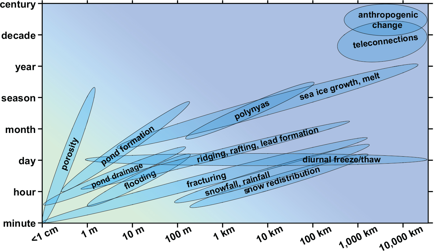
FIGURE 1. Examples of sea ice processes that occur over multiple spatial and temporal scales. The scales at which measurements are made often do not match the scales at which phenomena occur. The green background shading indicates scales over which in situ measurements are made, while the purple shading represents scales at which remote sensing retrievals are possible. Adapted from Blöschl and Sivapalan (1995) for the Arctic sea ice environment. > High res figure

 

As a case example, consider the relationship between snow depth and sea ice thickness in the Arctic in mid-spring. On point measurement scales (<0.5 m footprint), snow depth and the thickness of smooth sea ice beneath it are often negatively correlated, with locally thin sea ice having locally thick snow, and vice-versa. This inverse relationship arises due to snow’s high insulating capacity, which inhibits heat flux and sea ice growth (Sturm et al., 2002) and the greater susceptibility of wind-blown snow to be deposited in surface depressions, such as on top of refrozen melt ponds (see Figure 11d in Perovich et al., 2003).

In contrast, airborne retrievals of snow depth and sea ice thickness (Kurtz et al., 2015) show the opposite result. The airborne retrievals, as 40 m averages, yield a positive correlation between snow depth and sea ice thickness, meaning that on thicker ice, there is deeper snow, and vice versa. Although the two sets of observations seemingly contradict one another, both are correct for the spatial scales over which they are measured. Their differences underscore the importance of using the process scale to guide the interpretation of different observational scales (Blöschl and Sivapalan, 1995). Point measurements are effective in capturing local interactions and isolating mechanisms, making them central to gaining a deep understanding of physical processes and improving their representation in models; however, their broad-scale application across regions is limited.

Larger-scale measurements, such as airborne and satellite retrievals, are an integration of numerous processes, with large-scale processes having a stronger influence than small-scale processes. This can be readily seen in the pan-Arctic distribution of snow on Arctic sea ice (Webster et al., 2018). The deepest snow is found in regions with higher snowfall rates, older sea ice, and rougher sea ice. Unlike point measurements, larger-scale observations are better suited for monitoring pan-Arctic distributions and assessing the ability of Earth system models to simulate the cumulative effect of different processes on variables.

 

A Sample in Time

Temporal sampling of Arctic sea ice has greatly improved over the decades. Historically, most in situ measurements were made during spring-summer when the polar day permitted airborne surveys and landings on sea ice, and the summer retreat of ice allowed the passage of ships. From these early observations, weather patterns were quantified and related to patterns in sea ice drift around the Beaufort Gyre and along the Transpolar Drift Stream (Figure 2a). The discovery of the persistent Beaufort High in sea level pressure resulted from these observations.

 

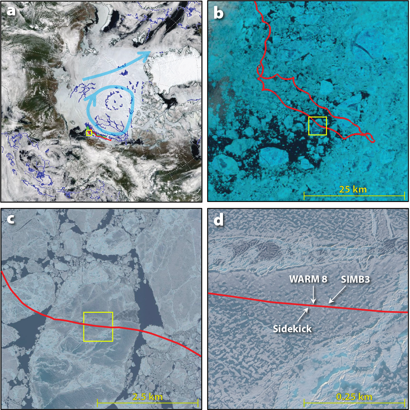
FIGURE 2. Maps of buoy drifts overlaid on satellite images of increasing resolution for June 2018. The yellow boxes indicate the areas zoomed-in from one figure panel to the next. (a) Blue dots show buoy positions for April 1–June 30, and the green and red lines show the drifts of buoy Clusters 1 and 2 during the same period, overlaid on a 1 km resolution MODIS true-color scene from June 22. The thick, light blue lines and arrows are schematics depicting the circulation of the Beaufort Gyre and the Transpolar Drift Stream. (b) The Cluster 2 drift overlaid on a 10 m resolution Sentinel-2 scene from June 24. (c) The Cluster 2 drift overlaid onto a ~0.4 m resolution WorldView-3 scene from June 28. (d) A WorldView-3 scene from June 28, where, upon closer inspection, individual buoys can be identified. ©2018 DigitalGlobe NextView License. > High res figure

 

Deployment of autonomous buoys (Polashenski et al., 2011; Lei et al., 2016; Wang et al., 2016; Perovich et al., 2021) and moored observatories (Spreen et al., 2020) enabled year-round observations of surface air pressure and temperature, upper ocean temperature and salinity, and other geophysical parameters. The temporal resolution of buoy observations was previously limited to the frequency of satellites passing overhead, resulting in sub-daily sampling on a timescale of synoptic atmospheric and oceanic processes. Now, with continuous coverage of the North Pole by Iridium, observations are considerably more frequent and can reveal short-lived processes. For example, hourly observations can capture the fracturing, ridging, and rafting of sea ice (Figures 2 and 3d), as well as the inertial oscillations in sea ice motion (Figure 2b). Processes that quickly thicken the ice relative to slow thermodynamic growth can readily be monitored by analyzing the areal geometric changes between buoy arrays over nested spatial scales (e.g., the Distributed Network in Nicolaus et al., 2022). Such high-frequency observations provide new opportunities for studying atmosphere-ice-ocean interactions: the impact of tides on sea ice surface roughness, the role of tides and wind-driven circulation in the evolution and distribution of sea ice thickness, and the influence of net divergence or convergence on geographic differences in summer melt processes, to name a few.

 

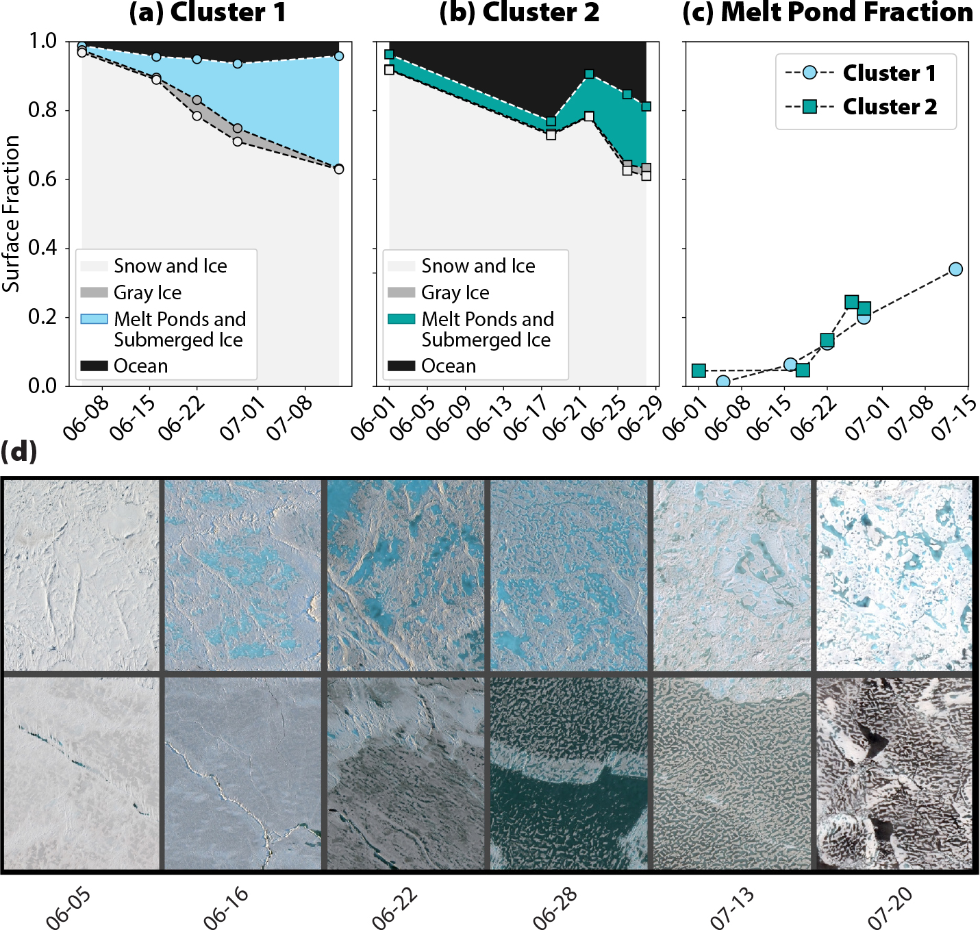
FIGURE 3. The evolution of the total areal surface fraction for (a) Cluster 1 and (b) Cluster 2. (c) The melt pond fraction, given as the ponded ice fraction. (d) A subset of pond evolution from WorldView images of Cluster 1. Panels in (d) show pond formation on multiyear (top row) and first-year (bottom row) ice. Each panel is 400 m x 400 m. Dates are presented as “month-day.” ©2018 DigitalGlobe NextView License. > High res figure

 

The amount of data transmitted by buoys has also increased dramatically, from a few bytes to hundreds of bytes. In the near future, the Iridium Certus system will enable the transmission of thousands of bytes. Together with higher data transmission, current electronics and batteries permit the collection of hourly observations. Further advances in low-power electronics and significant improvements in the power density of batteries have spurred initiatives within the World Meteorological Organization and Intergovernmental Oceanographic Commission to deploy buoys that transmit observations every 10 minutes.

 

Spatial Heterogeneity

The heterogeneity of Arctic sea ice is at its most vibrant display during the melt season. From May to September, the vast expanse of the snow-covered ice pack transforms into a mosaic of floes composed of bare and ponded sea ice. Melt ponds decrease the surface albedo and increase the amount of absorbed and transmitted sunlight (Perovich et al., 2002a). Features of the sea ice cover, like melt ponds, are highly variable in their spatial distribution, and they often change with time-varying processes. The scales over which these features change dictate the type of sensors that can be used to detect them and the frequency at which they can be sampled. For example, fully resolving individual melt ponds requires observing sea ice at the meter scale or finer. To capture pond drainage events, daily temporal resolution is needed at a minimum.

To explore spatial heterogeneity in sea ice observations, consider the evolution of melt ponds at the locations of two drifting buoy clusters in summer 2018 (Figures 2 and 3). Clusters 1 and 2 were tracked with high-resolution optical satellite (WorldView) imagery as they drifted across the Beaufort and Chukchi Seas. The images were analyzed using the open source sea ice processing algorithm (Wright and Polashenski, 2018) to detect the areal fraction of each image that falls into one of four surface categories: (1) snow and bare sea ice, (2) gray (thin or slushy) ice, (3) melt ponds or submerged ice, and (4) ocean.

Figure 3d shows a bird’s-eye view of the surface conditions. These subsets reveal how truly heterogeneous the Arctic sea ice cover can be on meter-to-kilometer scales. The smooth sea ice on the lower portion is representative of undeformed first-year sea ice, while the rougher, more variable surface in the upper portion is characteristic of multiyear sea ice. Both ice types coexist on the same floe, but the progression of melt ponding differs between the two. This arises from dissimilar surface roughness and ice permeability, which affects the areal coverage and persistence of melt ponds. Yet, even across floes of smooth first-year sea ice, there can be contrasting discrepancies in melt pond coverage, with widespread ponding on one floe and complete absence of ponds on another.

The different timing and distribution of melt ponds lead to locally variable rates of melt. If melt ponds form early in one location, that surface will undergo greater melt earlier in the season than unponded ice due to positive albedo feedback. If an area has larger melt ponds, its melt rate will be higher than that in areas with smaller melt ponds. At Cluster 1 (Figure 3d), melt pond formation began earlier on the multiyear ice portion. Despite this earlier formation, the melt ponding on the smooth, first-year ice was more extensive by late June in 2018, and the first-year ice soon deteriorated into a skeletal-like structure, full of holes where ponds once were. Shortly there­after, the first-year portion of the floe broke up, notably weeks earlier than the multiyear portion. When considering sea ice mass balance, whether the timing of formation or areal coverage of melt ponds is more important remains an open question, but this may be better understood with future coordinated tracking of drifting buoys by satellites.

Beyond the kilometer scale is the mesoscale (~10 km–1,000 km), a scale at which local heterogeneity starts to diminish and geographic differences and predominant sea ice conditions become increasingly important. Continuing with our melt pond example, we turn to the drifting buoy clusters to examine the scaling behavior of spatial heterogeneity. The two clusters remained ~150 km apart (Figure 2) as they drifted with the winds and ocean currents in May-August in 2018, and hence, they were subjected to similar synoptic conditions: similar snowfall, rainfall, temperatures, and radiative forcing. Accordingly, the average snow depths in their broader areas were alike, 0.19 m vs 0.18 m for Clusters 1 and 2, respectively. Even so, the physical state of the sea ice differed between the two clusters. In mid-April 2018, NASA’s Operation IceBridge airborne mission flew over both sites, measuring considerably thicker ice at Cluster 1 (2.2 ± 1.7 m), while Cluster 2 had relatively thinner sea ice (1.4 ± 1.1 m). Cluster 1’s location was also slightly northward and farther from the ice edge, which, together with having thicker ice, may have contributed to its longer survival during the melt season.

While there are some differences in the evolution of surface conditions between the two clusters at the 15 km × 15 km scale—notably that there was more open water and thinner, smoother sea ice at Cluster 2—the overall evolution of melt ponds was not significantly different between the two. These results, consistent with previous findings, reveal an important relationship between sea ice surface heterogeneity and scale: the coverage of melt ponds is highly variable across small spatial scales (tens of meters), but becomes increasingly consistent across larger scales (tens of kilometers) (Perovich et al., 2002b; Wright and Polashenski, 2018; and others). This phenomenon is known as the “aggregate scale,” or the scale at which the observed property is statistically representative of the larger region, and has been found to be tens of kilometers during the melt season (Perovich et al., 2002b). In essence, the local scale heterogeneity (Figure 3d; ~400 m × 400 m) collectively combines into a single aggregate scale (~15 km × 15 km) whose result reveals itself in the time series of the ponded ice fraction (Figure 3c).

 

Synthesizing Disparate Observations

Drifting buoys, moorings, and field campaigns typically have higher frequency sampling than air- and spaceborne missions, and the lower sampling frequency of satellite products limits their ability to detect short-lived events. In Figure 4, we combine disparate pieces of information to highlight the value of high frequency sampling and the advantages of co-​deploying complementary instruments, a common practice of collaborators in the International Arctic Buoy Programme (IABP; https://iabp.apl.uw.edu/). The data in Figure 4 come from several sources, including compiled data sets found in the Lagrangian ice parcel database (Horvath et al., 2021) and in ice mass balance (IMB; Perovich et al., 2021) and WArming and iRradiance Measurements (WARM; Hill et al., 2018) buoy data.

 

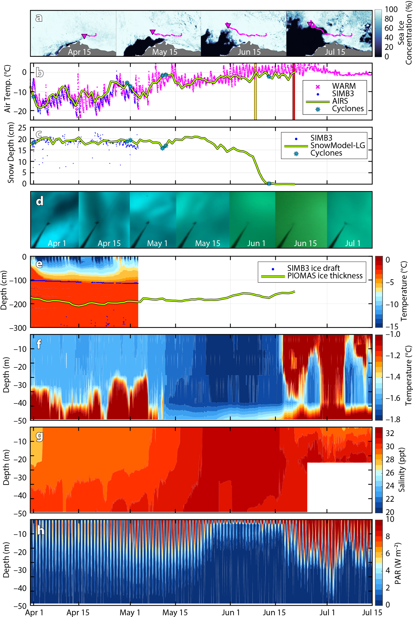
FIGURE 4. A compilation of satellite, model, and buoy data from Cluster 2 during 2018. (a) ARTIST Sea Ice (ASI) concentrations. (b) Air temperatures from the seasonal ice mass balance (SIMB), WArming and iRradiance Measurements (WARM) buoy, and derived by satellite (Atmospheric Infrared Sounder). Storm events are marked by cyan asterisks and satellite-derived dates of early onset (yellow) and continuous (red) melt by vertical bars. (c) Snow depth from the SIMB and Lagrangian snow-evolution model (SnowModel-LG). (d) Under-ice photos from the WARM buoy. (e) In-ice and ocean temperatures with ice drafts from the SIMB and simulated sea ice thickness from Pan-Arctic Ice-Ocean Modeling and Assimilation System (PIOMAS). (f) Ocean temperature from the WARM buoy. (g) Ocean salinity from the WARM buoy. (h) Photosynthetically active radiation (PAR) from the WARM buoy. > High res figure

 

In Figure 4b, consider the effects of temporal resolution on observed temperature. The buoy data exhibit a distinct diurnal cycling of temperatures, while the satellite-derived temperatures show a more slowly varying behavior and no diurnal cycling whatsoever. Different temporal sampling and different measurement techniques can produce substantially different results for the same phenomenon. The date of melt onset is an especially insightful example of the large differences that can arise between in situ and satellite-derived measurements (Figure 4b). In mid-May, in situ temperatures exceeded 0°C and surface melt was observed. Meanwhile, the satellite retrievals show a melt onset date three weeks later (Figure 3d). Deriving air temperature by satellite requires several assumptions, including those about emissivity, a property that is strongly influenced by the surface state and atmospheric water content (Ulaby et al., 1981; Jackson et al., 2006). Thus, discrepancies between in situ and satellite data sets can arise if assumptions in satellite retrievals do not truly reflect the ever-changing surface and atmospheric conditions. A three- to four-week discrepancy in the timing of melt onset changes the interpretation of cause and effect when it comes to interactions among the atmosphere, sea ice, and ocean, especially regarding primary productivity and melt processes.

And timing is everything for sea ice algae. Ice algae are a fundamental component of the Arctic marine food web (Kohlbach et al., 2016; Wiedmann et al., 2020) and are highly sensitive to the thickness of snow and sea ice due to their adaptation to low irradiance levels (Leu et al., 2015). At Cluster 2, the timing and duration of snow melt (Figure 4c) coincided with a notable ice algal bloom (Victoria Hill, Old Dominion University, pers. comm., 2021), resulting in less photosynthetically active radiation (PAR) in the upper ocean (Figure 4h). As melt pond formation progressed (Figure 3), irradiance levels returned to near-​normal levels. The ice algae bloom gradually diminished (Figure 4d), but it had left its mark: the long duration of low ocean PAR levels substantially disrupted phytoplankton productivity in the upper water column for the season (Victoria Hill, Old Dominion University, pers. comm., 2021).

Auxiliary information, such as ocean temperature and salinity (Figure 4f,g), provides added insight on potential nutrient loading and also on environmental conditions leading to abrupt sea ice changes. This case study illustrates how coordinated deployments enable single discipline and cross-discipline analyses, which can greatly aid system science investigations.

 

Scalability and its Impacts

One of the most powerful traits of Arctic sea ice is its high albedo, which results in reflection of ~40%–80% of solar radiation back into space, compared to only ~7% reflected by the open ocean (Perovich et al., 2011). Here, we estimate solar heat input into the ice-free and ice-covered Arctic Ocean to examine how small-scale heterogeneity manifests across spatial scales (Figure 5). We estimate solar heat input using a daily mean downwelling solar flux from ERA5 reanalysis (Hersbach et al., 2018), prescribed surface albedo as in Perovich et al. (2011), stages of melt and freeze onset dates derived from satellite data (Markus et al., 2009), and sea ice concentrations also derived from satellite data. This exercise was performed using three sea ice concentration retrievals, each covering a different spatial scale: WorldView (WV) ~15 km scene with ~0.4 m resolution (Figure 3), ARTIST Sea Ice (ASI) 6.25 km grid (Spreen et al., 2008), and Climate Data Record (CDR) 25 km grid (Meier et al., 2021).

 

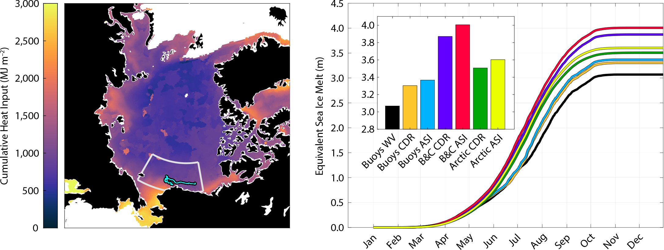
FIGURE 5. (left) Total annual solar heat input into the ice and ocean in 2018 from Climate Data Record (CDR) sea ice concentrations. Tracks of the drifting buoy clusters are drawn in cyan, and the region of the Beaufort and Chukchi Seas is outlined by the light gray box. (right) Equivalent amounts of sea ice melt based on the mean value of total annual solar heat input, an ice density of 900 kg m3, latent heat of fusion of 0.335 MJ km–1, and different sea ice concentration retrievals. Going from small to large scales, the estimates are derived from the buoy clusters (Buoys WV; Buoys CDR; Buoys ASI), the Beaufort and Chukchi Sea region (B&C CDR; B&C ASI), and the Arctic, averaged over 67°N–90°N (Arctic CDR; Arctic ASI). The inlaid bar chart displays the equivalent amounts of ice melt (meters) at the end of 2018. In reality, a small amount of heat would be lost through turbulent fluxes and other processes, and less ice melt would occur. B&C = Beaufort and Chukchi Sea region. ASI = ARTIST Sea Ice. CDR = Climate Data Record. WV = WorldView. > High res figure

 

First, consider the cumulative heat input on the smallest scale (6.25 km to 25 km) at the buoy clusters, where coincident pixels from the three sea ice concentration retrievals were evaluated (Figure 5, right: black, orange, and cyan lines). The estimates from the buoy clusters use the same solar flux and the same prescribed albedo for sea ice and open water; the differences arise solely from the sea ice concentrations, which are within ~1%–2% of one another throughout the year except for July, when ASI and CDR show 25% less sea ice coverage than the WV retrieval. The 25% difference in July sea ice coverage results in ~70–90 MJ m^–2 more heat going into the sea ice and open ocean. This is equivalent to ~0.2–0.3 m of additional sea ice melt in a region that had, on average, 1.7 m thick ice prior to melt onset.

There are several possibilities for the discrepancies in the solar heat input estimates. For one, the passive microwave retrievals (ASI, CDR) may erroneously detect melt ponds as open water. In the range of microwave electromagnetic radiation, melt ponds are sufficiently deep to mask the emissivity of the underlying sea ice and produce an emissivity similar to that of open ocean (Ulaby et al., 1981). Thus, the passive microwave retrievals may underestimate sea ice concentrations and overestimate solar absorption when melt ponds are present. Previous work (Rösel et al., 2012) suggests a low bias in passive microwave sea ice concentrations by as much as ~40% due to melt ponds. Approaches blending higher-resolution optical imagery with passive microwave may be a fruitful way forward in improving sea ice retrievals during the melt season, as the use of optical imagery alone is limited by clouds in summer.

Discrepancies in the estimated solar heat input could also stem from a sampling issue. Here, we examined grid cells of the satellite products at each buoy cluster, with the centers askew from one another. Moreover, the clusters are located in a markedly dynamic environment; the marginal ice zone is susceptible to large changes in ice coverage over relatively short periods, which can result in retrieval differences if satellites collect data at different times. To explore the differences in spatial resolution, we performed the same exercise using the ASI and CDR products on regional and pan-Arctic scales. The higher resolution product (ASI) yields more solar heat input (30 MJ m^–2) for both the Beaufort and Chukchi Sea regions and Arctic-wide. This equates to ~0.1 m of additional sea ice melt, which is distributed fairly uniformly across the Arctic, across ice concentrations, and between multiyear and first-year ice regions.

While there are significant differences between passive microwave products and their input data (Ivanova et al., 2015; Meier and Stewart, 2019), the differences in the solar heat input estimates shown here are still noteworthy. Collectively, they point to the need to continually revisit and refine remotely sensed sea ice observations as technology advances and our ability to resolve surface processes improves. Much like our understanding of the Arctic sea ice system, the techniques used to document sea ice conditions are ever-evolving, and there is added value in modernizing past observations to retain and reestablish a baseline from which long-term changes can be measured.

 

Auspicious Directions

Arctic sea ice loss is expected to continue over the next decades, with most model projections showing the first ice-free (extent under 1 million square kilometers) Arctic summer to occur by 2050 (Notz and SIMIP Community, 2020). As sea ice loss continues and technologies advance, autonomous systems and remote sensing will play increasingly larger roles in sea ice observations. As shown in the drifting cluster examples, harmonization between different observational scales and techniques augments the science that can be achieved with observational investments. Instrument arrays with complementary sensors are of particular interest since they enable cross-disciplinary science. They can capture the concomitant changes in atmospheric, sea ice, biological, and oceanic conditions, allowing for better understanding of processes on local scales. Coordinated airborne measurements and Lagrangian tracking of drifting arrays by satellite are at the forefront of sea ice observations. These types of observations provide the context necessary for relating local-scale heterogeneity and temporal variability to aggregate-scale properties and evolution. In particular, such fine-scale observations enable the scalability of in situ measurements for relating to coarse-resolution satellite products and model output.

Although future field operations may encounter greater risks with a thinner, less stable Arctic sea ice cover, in situ observation will be equally, if not more, valuable. As noted in Gerland et al. (2019), there are only a few clusters of ice and ocean buoys across Arctic sea ice at any given time, and there are recurring gaps in the observing network during winter when buoys drift into the Transpolar Drift Stream and away from the Eurasian coast. These gaps increase the uncertainties in our analyses of weather, sea ice, and climate change (Inoue et al., 2009; Inoue, 2021), and more efforts are needed to reseed the Arctic Observing Network during winter. Similarly, routine observations of sea ice conditions from ships initiated by the “Ice Watch” Arctic Shipborne Sea Ice Standardization Tool (ASSIST) Data Network (https://icewatch.met.no/) would benefit from the increasing number of ships operating in the Arctic.

New remote-sensing technologies, such as dual-sensor altimetry, will also require considerable ground validation programs to account for the anticipated environmental changes to come. The shift to seasonal, more saline sea ice, more frequent freeze-thaw cycling, and more frequent rainfall (Fox-Kemper et al., 2021) will lead to a more complex vertical substrate of snow and sea ice, posing greater challenges for remote-sensing retrievals in the future. To sufficiently quantify uncertainties and biases for scientific reliability, ground-truthing observations should optimally cover a wide range of snow and sea ice conditions. Ideally, such ground-truthing activities can be done in coordination with other observational efforts, such as drifting array deployments and planned field programs, including ecosystem studies, to foster collaboration and inclusivity across the broader community.

Lastly, models can optimize observations by helping guide observational priorities. Sensitivity experiments and observational assessments are effective in pinpointing sources of deficiencies in models, such as specific processes and physics. Targeting observations for such processes can help advance incomplete representations of heterogeneity, variability, and atmosphere-​ice-​ocean-​ecosystem interactions in models. Model inter-comparisons can elucidate regions and seasons where intra-model spread is large, and subsequently direct where and when observing systems are best placed. By bridging observational and modeling efforts, we can elevate the scientific, operational, and community return on investments, and better anticipate the cascading effects of the changing Arctic sea ice system.

 

Acknowledgments

We are especially grateful for the assistance of John Sonntag and Kyle Krabill from NASA’s Operation IceBridge team in coordinating overflights of field sites; James S. Hak from the United States Geological Survey and Mike Cloutier and Paul Morin from the University of Minnesota Polar Geospatial Center in acquiring co-located WorldView imagery; Cameron Planck from Cryosphere Innovation for his assistance in providing IMB data (Perovich et al., 2021); Don Perovich for his assistance in processing the IMB sonic range-finder data; and Sean Horvath for providing output of cyclone events, AIRS, SnowModel-LG, and PIOMAS from the Lagrangian ice parcel database (https://tc.copernicus.org/preprints/tc-2021-297/). WARM buoy data was obtained from the NSF Arctic Data Center. WorldView satellite imagery was provided with DigitalGlobe NextView License 2018 through the University of Minnesota Polar Geospatial Center. MODIS reflectance data (MYD09GA; Vermote, 2015) and Copernicus Sentinel-2 (ESA) reflectance data (10.5066/F76W992G) were acquired through the US Geological Survey. We thank two anonymous reviewers and Stephen Warren for their constructive reviews, which greatly improved the manuscript.

 

Funding

IR is funded by contributors to the US Interagency Arctic Buoy Program, which includes support from the US Coast Guard, Department of Energy, North Slope Borough, NASA (80NSSC21K1148), NOAA (NA15OAR4310154, and NA20OAR4320271), NSF (OPP-1951762), Office of Naval Research (N00014-20-1-2207), and USNIC. MW was funded by NASA’s Interdisciplinary Research in Earth Science program (80NSSC21K0264) and New Investigator Program in Earth Science (80NSSC20K0658). NW was funded by NASA’s Cryospheric Sciences Program (80HQTR21T0063).

Webster, M.A., I. Rigor, and N.C. Wright. 2022. Observing Arctic sea ice. Oceanography 35(3–4):28–37, https://doi.org/10.5670/oceanog.2022.115.

Abram, N.J., E.W. Wolff, and M.A.J. Curran. 2013. A review of sea ice proxy information from polar ice cores. Quaternary Science Review 79:168–183, https://doi.org/10.1016/j.quascirev.2013.01.011.

Barr, S., and C. Lüdecke, eds. 2010. The History of the International Polar Years (IPYs). Springer, Berlin, 320 pp., https://doi.org/10.1007/978-3-642-12402-0.

Blöschl, G., and M. Sivapalan. 1995. Scale issues in hydrological modelling: A review. Hydrological Processes 9:251–290, https://doi.org/10.1002/hyp.3360090305.

Divine, D.V., and C. Dick. 2006. Historical variability of sea ice edge position in the Nordic Seas. Journal of Geophysical Research 111(C1), https://doi.org/​10.1029/​2004JC002851.

Farrell, S.L., K. Duncan, E.M. Buckley, J. Richter-Menge, and R. Li. 2020. Mapping sea ice surface topography in high fidelity with ICESat-2. Geophysical Research Letters 47:e2020GL090708, https://doi.org/​10.1029/2020GL090708.

Fox-Kemper, B., H.T. Hewitt, C. Xiao, G. Aðalgeirsdóttir, S.S. Drijfhout, T.L. Edwards, N.R. Golledge, M. Hemer, R.E. Kopp, G. Krinner, and others. 2021. Ocean, cryosphere and sea level change. Chapter 9 in Climate Change 2021: The Physical Science Basis. Contribution of Working Group I to the Sixth Assessment Report of the Intergovernmental Panel on Climate Change. V. Masson-Delmotte, P. Zhai, A. Pirani, S.L. Connors, C. Péan, S. Berger, N. Caud, Y. Chen, L. Goldfarb, M.I. Gomis, M. Huang, K. Leitzell, E. Lonnoy, J.B.R. Matthews, T.K. Maycock, T. Waterfield, O. Yelekçi, R. Yu, and B. Zhou, eds, Cambridge University Press.

Fredensborg Hansen, R.M., E. Rinne, S.L. Farrell, and J. Skourup. 2021. Estimation of degree of sea ice ridging in the Bay of Bothnia based on geolocated photon heights from ICESat-2. The Cryosphere 15:2,511–2,529, https://doi.org/​10.5194/tc-15-2511-2021.

Frey, K.E., G.W.K. Moore, J.M. Grebmeier, and L.W. Cooper. 2015. Divergent patterns of recent sea ice cover across the Bering, Chukchi, and Beaufort Seas of the Pacific Arctic Region. Progress in Oceanography 136:32–49, https://doi.org/10.1016/​j.pocean.2015.05.009.

Gerland, S., D. Barber, W. Meier, C.J. Mundy, M. Holland, S. Kern, Z. Li, C. Michel, D.K. Perovich, and T. Tamura. 2019. Essential gaps and uncertainties in the understanding of the roles and functions of Arctic sea ice. Environmental Research Letters 14:043002, https://doi.org/​10.1088/1748-9326/ab09b3.

Gossett, J. 1996. Arctic research using nuclear submarines. Sea Technology 37(3):33–40.

Hersbach, H., B. Bell, P. Berrisford, G. Biavati, A. Horányi, J. Muñoz Sabater, J. Nicolas, C. Peubey, R. Radu, I. Rozum, and others. 2018. “ERA5 hourly data on pressure levels from 1979 to present.” Copernicus Climate Change Service (C3S) Climate Data Store (CDS), https://doi.org/10.24381/cds.bd0915c6.

Hill, V.J., B. Light, M. Steele, and R.C. Zimmerman. 2018. Light availability and phytoplankton growth beneath Arctic sea ice: Integrating observations and modeling. Journal of Geophysical Research: Oceans 123:3,651–3,667, https://doi.org/​10.1029/​2017JC013617.

Holmes, Q.A., D.R. Nuesch, and R.A. Shuchman. 1984. Textural analysis and real-time classification of sea-ice types using digital SAR data. IEEE Transactions on Geoscience and Remote Sensing GE-22(2):113–120, https://doi.org/10.1109/TGRS.1984.350602.

Horvath, S., L. Boisvert, C. Parker, M. Webster, P. Taylor, and R. Boeke. 2021. Fate of sea ice in the ‘New Arctic’: A database of daily Lagrangian Arctic sea ice parcel drift tracks with coincident ice and atmospheric conditions. The Cryosphere Discussions [preprint], https://doi.org/10.5194/tc-2021-297, in review.

Huntington, H.P., S. Gearheard, L. Kielsen Holm, G. Noongwook, M. Opie, and J. Sanguya. 2017. Sea ice is our beautiful garden: Indigenous perspectives on sea ice in the Arctic. Pp. 583–599 in Sea Ice. D.A. Thomas, ed., John Wiley and Sons, Ltd., https://doi.org/10.1002/9781118778371.ch25.

Inoue, J., T. Enomoto, T. Miyoshi, and S. Yamane. 2009. Impact of observations from Arctic drifting buoys on the reanalysis of surface fields. Geophysical Research Letters 36(8), https://doi.org/​10.1029/​2009GL037380.

Inoue, J. 2021. Review of forecast skills for weather and sea ice in supporting Arctic navigation. Polar Science 27:100523, https://doi.org/10.1016/j.polar.​2020.100523.

Ivanova, N., L.T. Pedersen, R.T. Tonboe, S. Kern, G. Heygster, T. Lavergne, A. Sørensen, R. Saldo, G. Dybkjær, L. Brucker, and M. Shokr. 2015. Inter-comparison and evaluation of sea ice algorithms: Towards further identification of challenges and optimal approach using passive microwave observations. The Cryosphere 9:1,797–1,817, https://doi.org/​10.5194/​tc-9-1797-2015.

Jackson, D.L., G.A. Wick, and J.J. Bates. 2006. Near-surface retrieval of air temperature and specific humidity using multisensor microwave satellite observations. Journal of Geophysical Research 111(D10), https://doi.org/​10.1029/​2005JD006431.

Ketchum, R.D. 1971. Airborne laser profiling of the Arctic pack ice. Remote Sensing of Environment 2:41–52, https://doi.org/​10.1016/​0034-4257(71)90076-9.

Kohlbach, D., M. Graeve, B.A. Lange, C. David, I. Peeken, and H. Flores. 2016. The importance of ice algae-produced carbon in the central Arctic Ocean ecosystem: Food web relationships revealed by lipid and stable isotope analyses. Limnology and Oceanography 61:2,027–2,044, https://doi.org/10.1002/lno.10351.

Kovacs, A., N.C. Valleau, and J.S. Holladay. 1987. Airborne electromagnetic sounding of sea-ice thickness and sub-ice bathymetry. Cold Regions Science and Technology 14:289–311, https://doi.org/​10.1016/0165-232X(87)90021-8.

Krupnik, I., C. Aporta, S. Gearheard, G. Laidler, and L. Kielsen, eds. 2010. Siku: Knowing Our Ice: Documenting Inuit Sea Ice Knowledge and Use. Springer, Dordrecht, 501 pp., https://doi.org/​10.1007/​978-90-481-8587-0.

Kurtz, N., M. Studinger, J. Harbeck, V. Onana, and D. Yi. 2015, updated 2019. “IceBridge Sea Ice Freeboard, Snow Depth, and Thickness Quick Look, Version 1.” 2018 subset, Boulder, Colorado USA, NASA National Snow and Ice Data Center Distributed Active Archive Center, https://doi.org/​10.5067/GRIXZ91DE0L9, accessed October 10, 2021.

Kwok, R. 2018. Arctic sea ice thickness, volume, and multiyear ice coverage: Losses and coupled variability (1958–2018). Environmental Research Letters 13:105005, https://doi.org/​10.1088/1748-9326/aae3ec.

Kwok, R., G. Cunningham, T. Markus, D. Hancock, J.H. Morison, S.P. Palm, S.L. Farrell, A. Ivanoff, J. Wimert, and the ICESat-2 Science Team. 2019. “ATLAS/ICESat-2 L3A Sea Ice Freeboard, Version 2.” Boulder, Colorado, USA, NASA National Snow and Ice Data Center Distributed Active Archive Center, https://doi.org/10.5067/ATLAS/ATL10.002, accessed in 2021.

Kwok, R., G. Cunningham, S. Kacimi, M. Webster, N. Kurtz, and A. Petty. 2020. Decay of the snow cover over Arctic sea ice from ICESat-2 acquisitions during summer melt in 2019. Geophysical Research Letters 47(12):e2020GL088209, https://doi.org/​10.1029/2020GL088209.

Lei, R., P. Heil, J. Wang, Z. Zhang, W. Li, and N. Li. 2016. Characterization of sea-ice kinematic in the Arctic outflow region using buoy data. Polar Research 35:22658, https://doi.org/10.3402/polar.v35.22658.

Leu, E., C.J. Mundy, P. Assmy, K. Campbell, T.M. Gabrielsen, M. Gosselin, T. Juul-Pedersen, and R. Gradinger. 2015. Arctic spring awakening—​Steering principles behind the phenology of vernal ice algae blooms. Progress in Oceanography 139:151–170, https://doi.org/10.1016/​j.pocean.2015.07.012

Markus, T., J.C. Stroeve, and J. Miller. 2009. Recent changes in Arctic sea ice melt onset, freezeup, and melt season length. Journal of Geophysical Research 114(C12), https://doi.org/​10.1029/​2009JC005436.

Meier, W.N., and J.S. Stewart. 2019. Assessing uncertainties in sea ice extent climate indicators. Environmental Research Letters 14:035005, https://doi.org/10.1088/1748-9326/aaf52c.

Meier, W.N., F. Fetterer, A.K. Windnagel, and J.S. Stewart. 2021. “NOAA/NSIDC Climate Data Record of Passive Microwave Sea Ice Concentration, Version 4.” 2018 subset, National Snow and Ice Data Center, Boulder, Colorado, https://doi.org/10.7265/efmz-2t65, accessed October 10, 2021.

Nansen, F., ed. 1902. The Norwegian North Polar Expedition, 1893–1896: Scientific Results. Pitman, London.

Nazintsev, Y.L. 1964. The heat balance of the surface of the multiyear ice cover in the central Arctic (in Russian). Trudy Arkticheskogo i Antarkticheskogo Nauchno-Issledovatel’skogo Instituta 267:110–126.

Nicolaus, M., D.K. Perovich, G. Spreen, M.A. Granskog, L. von Albedyll, M. Angelopoulos, P. Anhaus, S. Arndt, H.J. Belter, V. Bessonov, and others. 2022. Overview of the MOSAiC expedition: Snow and sea ice. Elementa: Science of the Anthropocene10 (1):000046, https://doi.org/10.1525/elementa.2021.000046.

Notz, D., and SIMIP Community. 2020. Arctic sea ice in CMIP6. Geophysical Research Letters 47:e2019GL086749, https://doi.org/​10.1029/2019GL086749.

Perovich, D.K., T.C. Grenfell, B. Light, and P.V. Hobbs. 2002a. Seasonal evolution of the albedo of multiyear Arctic sea ice. Journal of Geophysical Research 107(C10), https://doi.org/​10.1029/2000JC000438.

Perovich, D.K., W.B. Tucker III, and K.A. Ligett. 2002b. Aerial observations of the evolution of ice surface conditions during summer. Journal of Geophysical Research 107(C10), https://doi.org/​10.1029/2000JC000449.

Perovich, D.K., T.C. Grenfell, J.A. Richter-Menge, B. Light, W.B. Tucker III, and H. Eicken. 2003. Thin and thinner: Sea ice mass balance measurements during SHEBA. Journal of Geophysical Research 108(C3), https://doi.org/​10.1029/​2001JC001079.

Perovich, D.K., K.F. Jones, B. Light, H. Eicken, T. Markus, J. Stroeve, and R. Lindsay. 2011. Solar partitioning in a changing Arctic sea-ice cover. Annals of Glaciology 52(57):192–196.

Perovich, D., J. Richter-Menge, and C. Polashenski. 2021. “Observing and understanding climate change: Monitoring the mass balance, motion, and thickness of Arctic sea ice,” http://imb-crrel-dartmouth.org/.

Polashenski, C., D. Perovich, J. Richter-Menge, and B. Elder. 2011. Seasonal ice mass-balance buoys: Adapting tools to the changing Arctic. Annals of Glaciology 52(57):18–26, https://doi.org/​10.3189/​172756411795931516.

Polyak, L., R.B. Alley, J.T. Andrews, J. Brigham-Grette, T.M. Cronin, D.A. Darby, A.S. Dyke, J.J. Fitzpatrick, S. Funder, M. Holland, and others. 2010. History of sea ice in the Arctic. Quaternary Science Review 29(15–16):1,757–1,778, https://doi.org/​10.1016/​j.quascirev.2010.02.010.

Reiser, F., S. Willmes, and G. Heinemann. 2020. A new algorithm for daily sea ice lead identification in the Arctic and Antarctic winter from thermal-​infrared satellite imagery. Remote Sensing 12(12):1957, https://doi.org/10.3390/rs12121957.

Ricker, R., S. Hendricks, L. Kaleschke, X. Tian-Kunze, J. King, and C. Haas. 2017. A weekly Arctic sea-ice thickness data record from merged CryoSat-2 and SMOS satellite data. The Cryosphere 11:1,607–1,623, https://doi.org/​10.5194/tc-11-1607-2017.

Romanov, I.P. 1995. Atlas of Ice and Snow of the Arctic Basin and Siberian Shelf Seas, 2nd ed. Translated from Russian by A. Tunik, Backbone, Paramus, NJ.

Rösel, A., L. Kaleschke, and G. Birnbaum. 2012. Melt ponds on Arctic sea ice determined from MODIS satellite data using an artificial neuronal network. The Cryosphere 6:1–19, https://doi.org/10.5194/tc-6-431-2012.

Rostosky, P., G. Spreen, S.L. Farrell, T. Frost, G. Heygster, and C. Melsheimer. 2018. Snow depth retrieval on Arctic sea ice from passive microwave radiometers—Improvements and extensions to multiyear ice using lower frequencies. Journal of Geophysical Research: Oceans 123:7,120–7,138, https://doi.org/10.1029/2018JC014028.

Spreen, G., L. Kaleschke, and G. Heygster. 2008. Sea ice remote sensing using AMSR-E 89-GHz channels. Journal of Geophysical Research 113(C2), https://doi.org/10.1029/2005JC003384.

Spreen, G., L. de Steur, D. Divine, E. Hansen, S. Gerland, and R. Kwok. 2020. “Fram Strait Sea Ice Volume Transport Based on ULS Ice Thickness and Satellite Ice Drift.” Data set published by the Norwegian Polar Institute, https://doi.org/10.21334/npolar.2020.696b80db.

Sturm, M., D.K. Perovich, and J. Holmgren. 2002. Thermal conductivity and heat transfer through the snow on the ice of the Beaufort Sea. Journal of Geophysical Research: Oceans 107(C21), https://doi.org/​10.1029/2000JC000409.

Thorndike, A.S., and R. Colony. 1982. Sea ice motion in response to geostrophic winds. Journal of Geophysical Research: Oceans 87(C8):5,845–5,852, https://doi.org/​10.1029/JC087iC08p05845.

Tschudi, M.A., W.N., Meier, and J.S. Stewart. 2020. An enhancement to sea ice motion and age products at the National Snow and Ice Data Center (NSIDC). The Cryosphere 14:1,519–1,536, https://doi.org/​10.5194/tc-14-1519-2020.

Vermote, E. 2015. “MOD09A1, v006, MODIS/Aqua Surface Reflectance 8-Day L3 Global 500m SIN Grid.” NASA EOSDIS Land Processes DAAC, https://doi.org/​10.5067/MODIS/MYD09A1.006.

Ulaby, F.T., M.K. Moore, and A.K. Fung. 1981. Microwave Remote Sensing: Active and Passive: Fundamentals and Radiometry, vol. I. Addison-Wesley, Boston, MA, 456 pp.

Walsh, J.E., F. Fetterer, J.S. Stewart, and W.L. Chapman. 2016. A database for depicting Arctic sea ice variations back to 1850. Geographical Review 107(1):89–107, https://doi.org/​10.1111/​j.1931-0846.2016.12195.x.

Wang, C., M.A. Granskog, S.R. Hudson, S. Gerland, A.K. Pavlov, D.K. Perovich, and M. Nicolaus. 2016. Atmospheric conditions in the central Arctic Ocean through the melt seasons of 2012 and 2013: Impact on surface conditions and solar energy deposition into the ice-ocean system. Journal of Geophysical Research: Atmospheres 121:1,043–1,058, https://doi.org/​10.1002/2015JD023712.

Warren, S., I. Rigor, N. Untersteiner, V.F. Radionov, N.N. Bryazgin, Y.I. Aleksandrov, and R. Colony. 1999. Snow depth on Arctic sea ice. Journal of Climate 12:1,814–1,829, https://doi.org/10.1175/1520-0442(1999)012​<1814:SDOASI>2.0.CO;2.

Webster, M.A., I.G. Rigor, S.V. Nghiem, N.T. Kurtz, S.L. Farrell, D.K. Perovich, and M. Sturm. 2014. Interdecadal changes in snow depth on Arctic sea ice, Journal of Geophysical Research: Oceans 119:5,395–5,406, https://doi.org/​10.1002/2014JC009985.

Webster, M.A., S. Gerland, M. Holland, E. Hunke, R. Kwok, O. Lecomte, R. Massom, D. Perovich, and M. Sturm. 2018. Snow in the changing sea-ice systems. Nature Climate Change 8:946–953, https://doi.org/​10.1038/s41558-018-0286-7.

Wiedmann, I., E. Ershova, B.A. Bluhm, E.M. Nöthig, R.R. Gradinger, K. Kosobokova, and A. Boetius. 2020. What feeds the benthos in the Arctic Basins? Assembling a carbon budget for the deep Arctic Ocean. Frontiers in Marine Science 7:224, https://doi.org/10.3389/fmars.2020.00224.

Wright, N., and C. Polashenski. 2018. Open-source algorithm for detecting sea ice surface features in high-resolution optical imagery. The Cryosphere 12(4):1,307–1,329, https://doi.org/​10.5194/tc-12-1307-2018.

This is an open access article made available under the terms of the Creative Commons Attribution 4.0 International License (https://creativecommons.org/licenses/by/4.0/), which permits use, sharing, adaptation, distribution, and reproduction in any medium or format as long as users cite the materials appropriately, provide a link to the Creative Commons license, and indicate the changes that were made to the original content. Images, animations, videos, or other third-party material used in articles are included in the Creative Commons license unless indicated otherwise in a credit line to the material. If the material is not included in the article’s Creative Commons license, users will need to obtain permission directly from the license holder to reproduce the material.