Sea surface salinity (SSS) is among the key indicators of air-sea buoyancy fluxes and the global hydrological cycle. Contributing to the second phase of the Salinity Processes in the Upper-ocean Regional Study (SPURS-2) carried out in the precipitation-dominated Intertropical Convergence Zone of the eastern Pacific, we deployed six Lagrangian drifters equipped with two pairs of temperature and conductivity sensors at 0.4 m and 5 m depth. Over the first three months, the drifter measurements revealed that (1) the wind strongly affects surface freshening resulting from rainfall and diurnal warming so that near-surface salinity and temperature gradients generally do not form at wind speeds greater than 7 m s^–1, (2) temperature and salinity differences between the two measurement depths are positively correlated for the cases of surface warming/salinification and freshening/cooling, (3) the lifetimes of rain-induced salinity anomalies can reach 24 hours, longer than previous estimates, (4) temperature (at 0.4 m and 5 m depth) and salinity (at 0.4 m depth) exhibit diurnal cycles, modulated by the wind, and (5) the differences that have been observed between satellite SSS and the standard uppermost salinity from Argo measurements are unlikely to be related to the difference in measurement depths (surface skin layer vs ~5 m depth).

 

A dual-sensor drifter just deployed in its biodegradable box from R/V Roger Revelle on August 24, 2016. The box degrades in a few hours and the drifter releases. Small-scale rain can be seen on the horizon. Photo credit: D.L. Volkov. > High res figure

Introduction

Despite the importance of sea surface salinity (SSS) as an indicator of the hydrological cycle (Rhein et al., 2013), many details of air-sea interaction responsible for freshwater fluxes and processes that determine near-surface salinity stratification and its variability are still poorly understood. This limited knowledge is primarily due to a lack of dedicated observations. Historically, salinity and temperature have been measured during hydrographic surveys. Since the early 2000s, Argo floats have provided regular, nearly global (achieved in 2005) measurements of these parameters in the upper 2,000 m of the water column. The downsides of both the ship-borne CTD and Argo measurements are their coarse spatial and temporal sampling, and most are limited to depths greater than 5 m. This means that the near-surface temperature and salinity stratification due to fresh­water fluxes cannot be measured with these tools. Furthermore, rain puddles in the ocean are transient, small-scale, shallow (a few meters), and patchy structures, sensitive to the ship wake, which complicates their observation even more.

The advent of satellites capable of monitoring SSS, such as the Soil Moisture and Ocean Salinity (SMOS; Kerr et al., 2010), Aquarius (Lagerloef et al., 2008), and Soil Moisture Active Passive (SMAP; Fore et al., 2016) missions, has greatly advanced our knowledge of SSS distribution and variability globally. However, the spatial resolution of satellite retrievals is too coarse to study the upper-ocean salinity changes caused by transient rain events. In addition, the satellites measure salinity within the upper 0.01 m skin layer, which can differ significantly from salinity at 5 m depth. Dong et al. (2017) reported differences between Aquarius SSS and Argo 5 m salinity as large as ±0.5 psu. This could be due to the different measurement depths (~0.01 m and 5 m), different temporal and spatial sampling, and biases in satellite SSS retrieval, among others. Freshening in the upper few meters due to rainfall events can easily exceed 1 psu (Drushka et al., 2016) and, therefore, can significantly contribute to the observed differences between satellite and Argo salinity data in regions of strong precipitation (Boutin et al., 2016). Freshening can also favor shallow temperature stratification and limit the depth of convection and wind stirring (Grodsky et al., 2008).

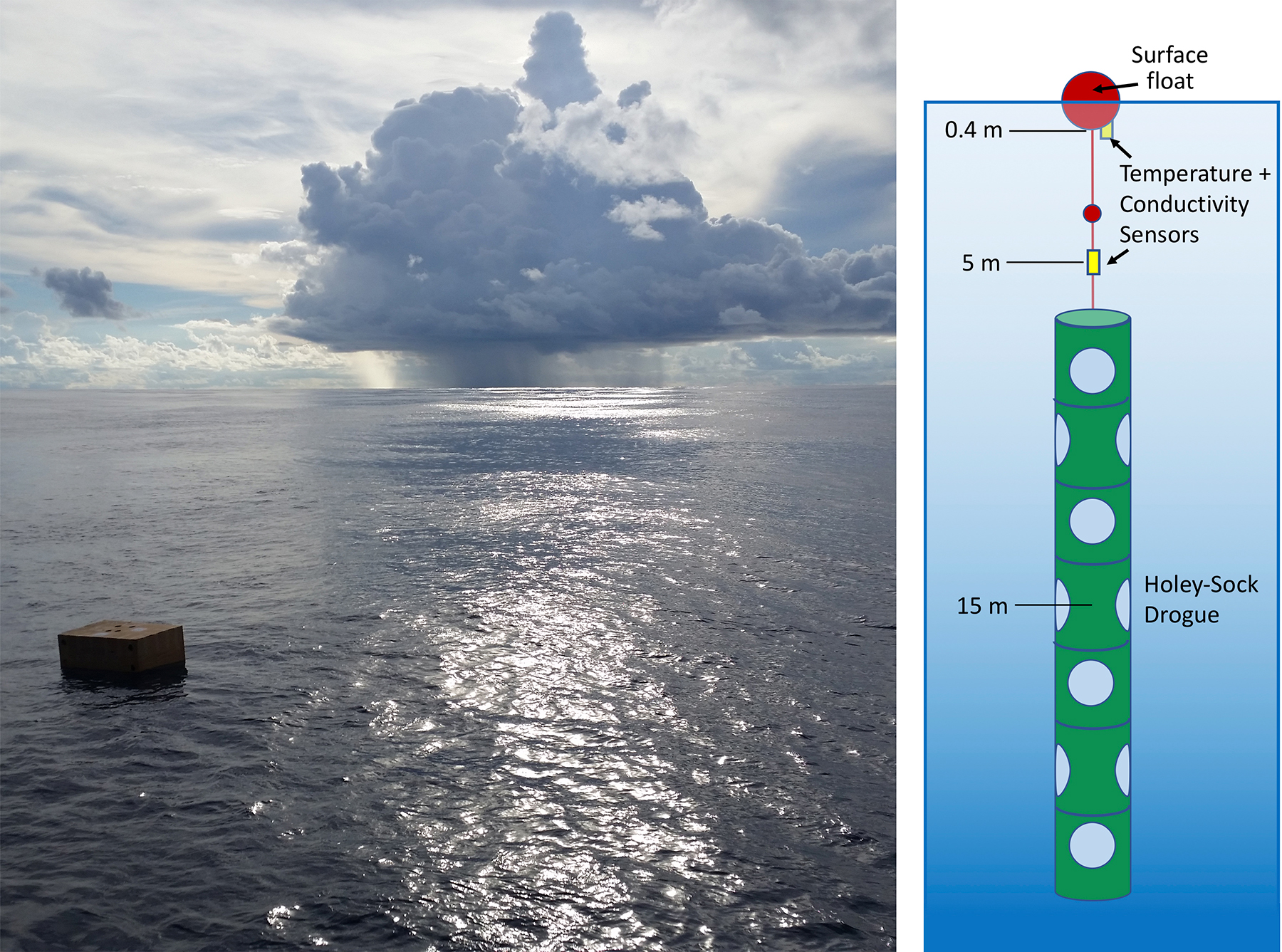
In order to study near-surface salinity structure in great detail and to link satellite observations of SSS with all the oceanic and atmospheric processes that control its variability, NASA initiated two field campaigns within the framework of the Salinity Processes in the Upper-ocean Regional Study (SPURS) project (https://spurs.jpl.nasa.gov/). The first campaign, SPURS-1, took place in the evaporation-​dominated subtropical North Atlantic Ocean in 2012–2013. The second campaign, SPURS-2, focused on a 3° × 3° domain in the Intertropical Convergence Zone (ITCZ) in the eastern equatorial Pacific (123.5°–126.5°W and 8.5°–11.5°N; Figure 1a,b), where the near-surface salinity is strongly dominated by precipitation. During the first SPURS-2 cruise in August–September 2016 aboard R/V Roger Revelle, a complex multi-instrument oceanographic survey was conducted (Lindstrom et al., 2017).

 

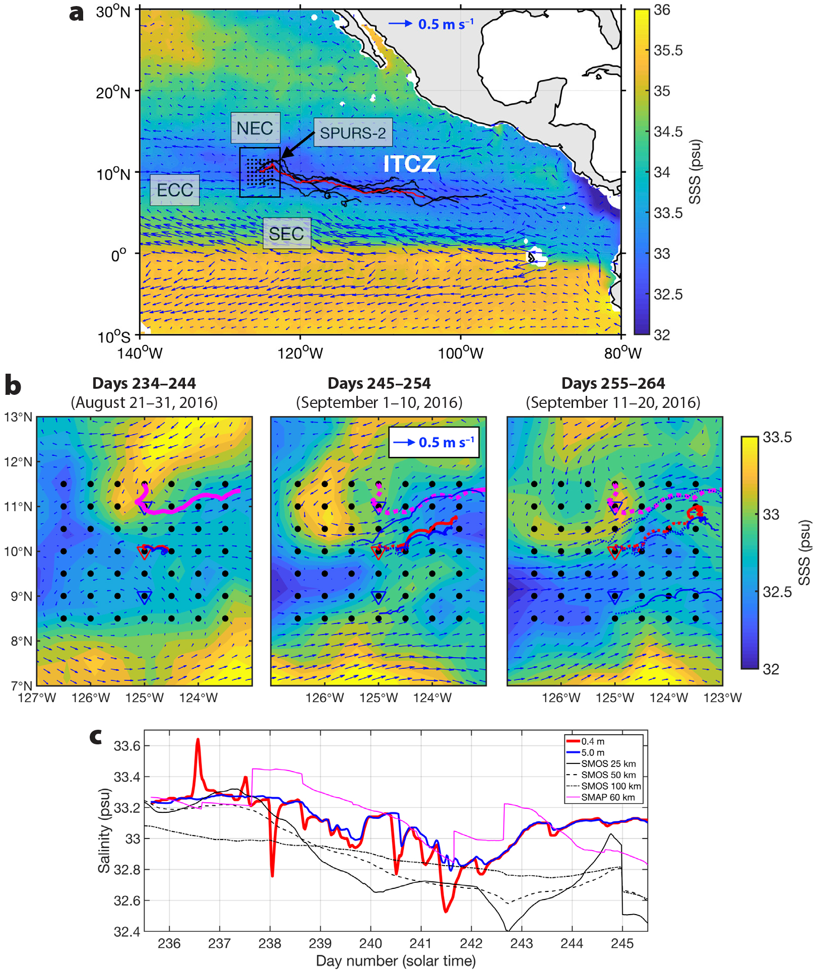
Figure 1. (a) Map of the eastern equatorial Pacific with the August–November 2016 mean sea surface salinity (SSS) measured by the Soil Moisture Active Passive (SMAP; color) satellite and the trajectories of six NOAA-AOML dual-sensor salinity drifters in August–November 2016 (curves). (b) Ten-day averages of SSS measured by the Soil Moisture and Ocean Salinity (SMOS) satellite from August 21, 2016, to September 20, 2016, (color) and drifter trajectories (curves). Dashed curves show trajectories for the past 10-day time intervals, while solid segments show trajectories over the current 10-day time interval. The trajectory of drifter #145718, whose records are shown in Figure 2a–d, is shown by red curves. (c) The records of salinity at 0.4 m (red) and 5 m (blue) depths by drifter #145738, whose trajectory is shown by magenta curves in Figure 1b. The SSS data from SMOS and SMAP interpolated on the drifter positions in space and time are shown by black and magenta curves, respectively. SMOS data are shown for 25 km (solid), 50 km (dashed), and 100 km (dashed-​dotted) resolutions. In (a) and (b), SPURS-2 stations/moorings are shown by dots/​triangles. Arrows show the OSCAR surface velocities averaged over the study interval (August–November 2016) in (a), and over 10-day time intervals in (b). NEC = North Equatorial Current. ECC = North Equatorial Countercurrent. SEC = South Equatorial Current. ITCZ = Intertropical Convergence Zone. > High res figure

 

As part of this field campaign, NASA and NOAA’s Atlantic Oceanographic and Meteorological Laboratory (AOML) supported the deployment of six dual-sensor Lagrangian drifters that were specifically designed to measure temperature and salinity near the surface (~0.4 m) and at 5 m depth (in waveless conditions). This deployment complemented the other types of near-surface salinity measurements obtained during the cruise, both autonomous (Lindstrom et al., 2017) and ship-based, for example, with Wave Gliders (Hodges and Fratantoni, 2014), a surface salinity profiler (SSP; Asher et al., 2014a), and a salinity snake (Schanze et al., 2014). The main objectives of this deployment were (1) to explore salinity stratification in the upper 5 m and processes that determine it, in particular in relation to rain events, and (2) to provide an observational benchmark for validating satellite SSS retrievals in precipitation-​dominated regions. In this paper, we report on these unique observations and present science results with respect to the objectives of the deployment.

 

Observations with Dual-Sensor Drifters

For this experiment, we used specially designed SVP-S (Surface Velocity Program – Salinity) drifters manufactured by Pacific Gyre (https://www.pacificgyre.com). The same drifters were deployed earlier in the subtropical South Pacific (Dong et al., 2017). Each drifter was equipped with a battery pack, a satellite transmitter, and two sets of conductivity/​temperature sensors: one (SBE-37SI) was mounted to the bottom of an upgraded (46 cm in diameter) surface float to avoid direct radiative heating, and the other was tether-mounted at 5 m depth (SBE-37SM). The SBE-37SI instrument was mounted vertically in a cylindrical cover about 32 cm long, with temperature and salinity sensors collocated roughly at the center of the cover. In waveless conditions, the float sits in the water at its equator, putting the upper sensors about 0.4 m below the surface. The accuracies of the conductivity and temperature sensors are ±3 × 10^-4 S m^–1 (approximately ±3 × 10^–3 psu) and ±2 × 10^–3 °C, respectively. The sampling interval was about 30 minutes. The drifters each had a standard Global Drifter Program-style holey-sock drogue centered at 15 m to follow currents at this depth. Each drifter was packed and deployed in a biodegradable box that allowed proper deployment of the drogue, tether, and surface float. For the study presented here, in order to focus on the conditions similar to those in the SPURS-2 domain, we used only about three months of drifter records starting from the times of deployment (Table 1) to the beginning of December 2016. The drifter records were cleaned for outliers in temperature, salinity, and geolocation data.

 

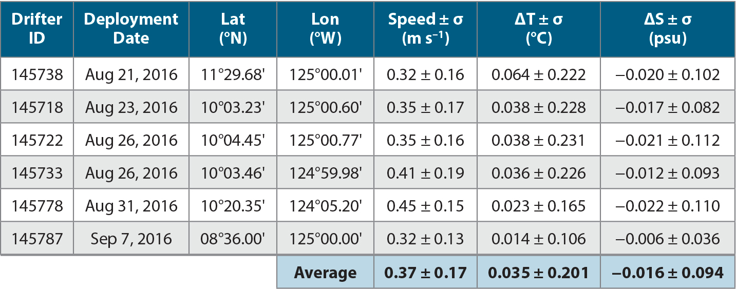
Table 1. The identification numbers of dual-sensor drifters; dates and locations of their deployments in the SPURS-2 region; average speeds of drifters, and average temperature and salinity differences between 0.4 m and 5.0 m depth over the first ~3 months after deployment. The variability of each measurement is shown by one standard deviation (σ). The averages are weighted by the number of valid measurements available from each drifter. > High res table

 

Table 1 displays the drifter identification numbers, dates and locations of deployment, and the average temperature (∆T = ∆T_0.4 − ∆T_5.0) and salinity (∆S = ∆S_0.4 − ∆S_5.0) differences between 0.4 m and 5 m depth, as well as their standard deviations. The first drifter (ID number 145738) was deployed at the northern boundary of the SPURS-2 domain (Figure 2b); three drifters (#145718, #145722, #145733) were deployed in a cluster near the central SPURS-2 mooring (the red triangle in Figure 1b); one drifter (#145778) was deployed near the southern boundary of the SPURS-2 domain; and the last drifter (#145787) was deployed about a half-degree west of the central mooring. As demonstrated by the time-mean (August through November 2016) field of SSS from SMAP and drifter trajectories during the first three months after the deployment, all six drifters stayed within the low-salinity ITCZ and were carried eastward by the North Equatorial Countercurrent (NECC) heading toward the equatorial Pacific SSS minimum off the coast of Central America (Figure 1a). The drifters moved with average speeds of 0.3–0.4 m s^–1 (Table 1), in good agreement with ⅓° resolution OSCAR (Ocean Surface Current Analysis Real-time) near-surface currents (Figure 1a,b).

 

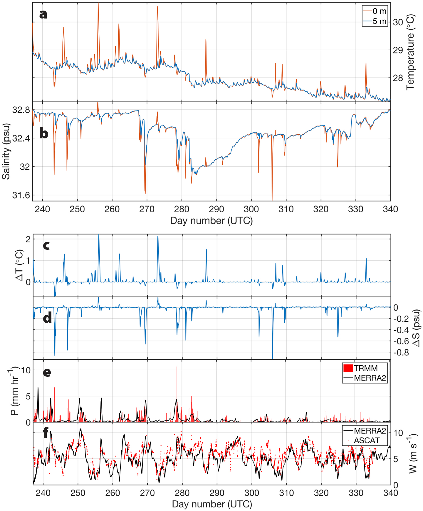
Figure 2. (a) Temperature and (b) salinity records from drifter #145718 at 0.4 m (red curves) and at 5 m (blue curves) depths; differences between (c) temperature and (d) salinity measurements at the two depths; and concurrent estimates of (e) precipitation (red bars) from Tropical Rainfall Measuring Mission (TRMM) and (black) Modern-Era Retrospective Analysis for Research and Application version 2 (MERRA-2) reanalysis, and (f) wind speed from (red dots) the Advanced Scatterometer (ASCAT) and (black) MERRA-2 reanalysis. > High res figure

 

The drifter trajectories and records were influenced by mesoscale features, mostly associated with westward-​propagating signatures of tropical instability waves. For example, drifter #145738 was deployed in a positive salinity anomaly, as evidenced by concurrent measurements from SMOS (Figure 1b). This anomaly was associated with a cyclonic circulation that initially carried the drifter southward toward the northern SPURS-2 mooring. As the salinity anomaly propagated westward, the drifter moved to a lower salinity region on days 240–241. This is well supported by both satellite and drifter salinity records (Figure 1b,c). Besides this gradual change of salinity, the drifter records also show short-term fluctuations caused by (1) the diurnal cycle at the beginning of the record (days 236–237), and (2) rain events (days 238–241).

Figure 2a,b displays the temperature and salinity records for drifter #145718 for the period considered in this study (the drifter trajectory is highlighted in Figure 1a,b). Similar records were obtained for all six drifters. As the drifters moved eastward-southeastward, the temperature at both depth levels (0.4 m and 5 m) gradually decreased by about 1°–2°C (Figure 2a), subject to diurnal fluctuations that were more pronounced at the surface. The average ∆T for all drifters is 0.035°C with a standard deviation of 0.201°C (Figure 2c, Table 1). The positive temperature difference and its relatively large standard deviation are due to irregular strong diurnal signals at 0.4 m compared to 5 m depth. Salinity changes were mostly due to transient mesoscale features and rain events (Figure 2b). Frequent rain events in the region are responsible for the negative average ∆S of −0.016 psu with a standard deviation of 0.094 psu (Figure 2d, Table 1).

 

Impact of Precipitation and Wind

To investigate the impact of atmospheric forcing on the near-surface temperature and salinity stratification, the drifter records were compared to observed and modeled precipitation and wind data. Satellite observations of rain used in this study are the output from the TRMM (Tropical Rainfall Measuring Mission) Multi-​satellite Precipitation Algorithm (TPMA), provided by the Goddard Distributed Active Archive Center on a 0.25° × 0.25° grid and at three-hour temporal resolution (Huffman et al., 2010; TRMM, 2011; https://disc.gsfc.nasa.gov/). Satellite measurements of wind speed were obtained from the 12.5 km resolution Advanced Scatterometer (ASCAT) Level 2 Wind Product generated through the processing of reprocessed scatterometer backscatter data originating from the ASCAT instrument on EUMETSAT’s Metop satellite (EUMETSAT, 2016). In addition, both precipitation and wind speed data were obtained from the Modern-Era Retrospective Analysis for Research and Application version 2 (MERRA-2) product (GMAO, 2015). The MERRA-2 is a NASA atmospheric reanalysis for the satellite era using the Goddard Earth Observing System Model, Version 5 (GEOS-5) with its Atmospheric Data Assimilation System, available on a 0.5° × 0.625° grid with one-hour temporal resolution. The precipitation and wind data have been linearly interpolated onto the locations and times of the drifter measurements (Figure 2e,d).

Overall, there is a reasonable correspondence between the negative ∆S and rain events (Figure 2e). The observed ∆S is better correlated with the satellite-​derived precipitation from TRMM (r = −0.3) than with the MERRA-2 precipitation (r = −0.1). Although the TRMM data are assimilated in MERRA-2, not all rain events present in TRMM are reproduced by MERRA-2. The correlation between the TRMM and MERRA-2 precipitation data interpolated onto the locations of drifter measurements is 0.37. The large scatter between ∆S and TRMM precipitation rates (Figure 3d) illustrates that the relationship is hardly linear. A similar result has been obtained with identical drifters in the subtropical South Pacific (Dong et al., 2017), and with regular SVP-S drifters measuring conductivity and temperature at ~45 cm depth deployed in the Atlantic and South Pacific (Boutin et al., 2014). This is probably because of the differences in sampling and the local influence of wind. In contrast, a quasi-linear dependence between ∆S and precipitation has been established using only satellite products of SSS and rain rate (e.g., Boutin et al., 2013; Supply et al., 2017). It is important to note that satellite precipitation products represent averages over the satellite footprint, while drifters provide point measurements. Because rainfall events are small scale and patchy, it is not surprising that significant salinity differences between the drifter measurement depths do not always coincide with precipitation data.

 

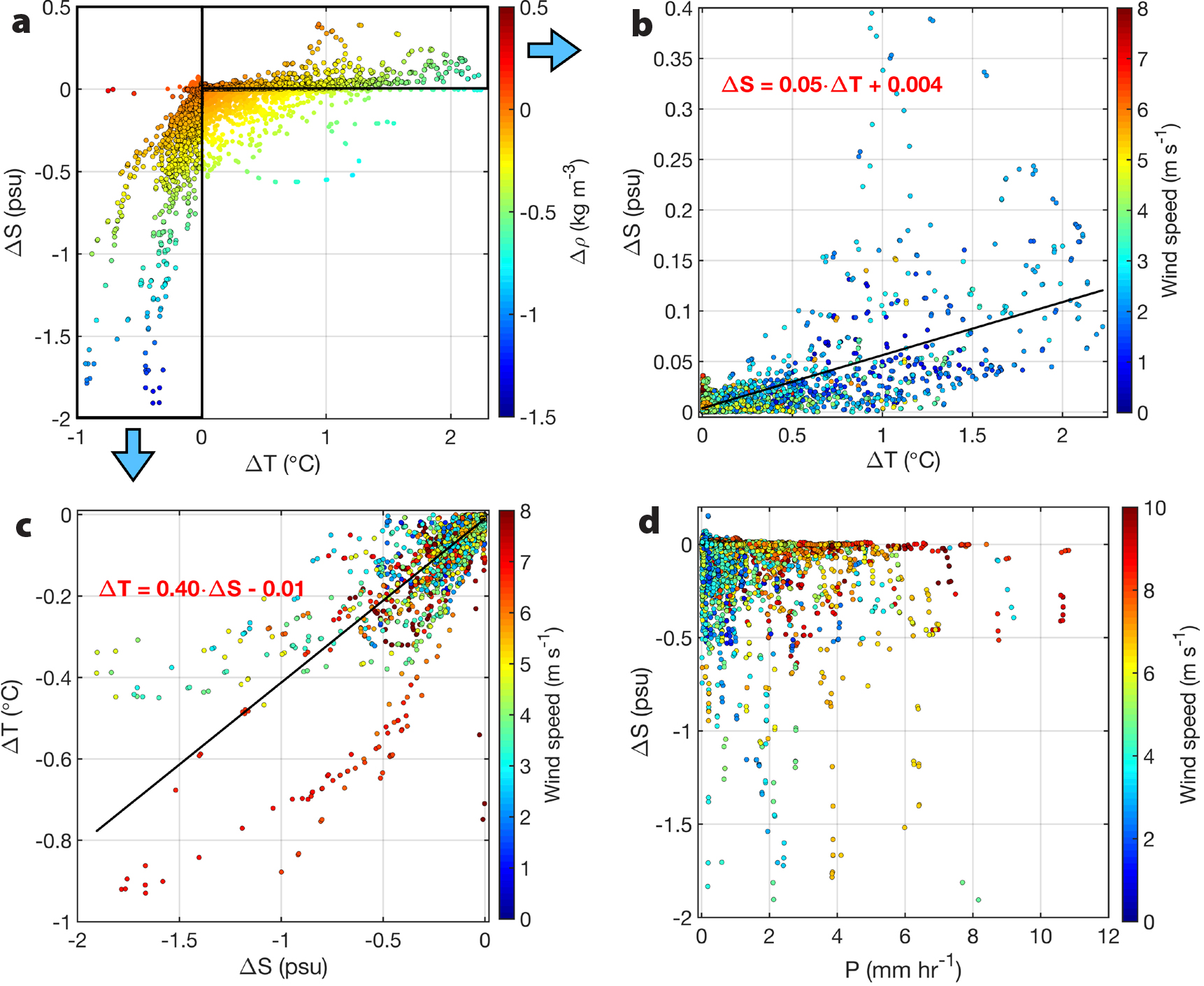
Figure 3. (a) Scatter of temperature (∆T) and salinity (∆S) differences between 0.4 m and 5 m depths with color showing the associated density differences. (b) Same as (a), but for the positive ∆T and ∆S with the black line showing regression of ∆S on ∆T. (c) Same as (a), but for the negative ∆S and ∆T with the black line showing regression of ∆T on ∆S. (d) Scatter of precipitation from TRMM and ∆S. Color in (b–d) shows the MERRA-2 wind speed. > High res figure

 

There is a much better match between the MERRA-2 winds and ASCAT winds, which are assimilated in MERRA-2 (Figure 2f). The correlation between the two wind products along the drifter trajectories is 0.65. The largest salinity differences between 0.4 m and 5 m depths generally occur when wind speeds are less than about 7 m s^–1 (Figures 2f and 3d) and precipitation is below 5 mm hr^–1 (Figure 3d). This is due to the fact that stronger rainfall is usually associated with stronger winds that enhance mixing and, thus, reduce or eliminate near-​surface stratification. The salinity differences are generally small (less than ±0.5 psu) at wind speeds ≥8 m s^–1, even for strong precipitation. There are only a few cases in which rather strong precipitation from 4 mm hr^–1 to 7 mm hr^–1 induces ∆S <−1 psu at wind speeds of about 7 m s^–1.

Assuming that ∆S of less than −0.05 psu in the drifter data is representative of rainfall, we identified 95 rain events during the first three months of drifter observations. Among them, 75 events were associated with −0.5 < ∆S ≤ −0.05 and only 20 with −2.0 ≤ ∆S < −0.5. Figure 4 displays the composites of salinity (c,d) and temperature (e,f) at 0.4 m and 5 m depth, as well as TRMM precipitation and MERRA-2 wind speed (a,b) for the two ∆S ranges, centered at the minimum ∆S. The maximum TRMM precipitation is about 1 ± 0.3 mm hr^–1 for −0.5 < ∆S ≤ −0.05, and it doubles (2.2 ± 1.0 mm hr^–1) for −2.0 ≤ ∆S < −0.5. It can be noted that TRMM precipitation is non-zero one day prior and one day after the maximum. This is probably due to the limited spatial and temporal resolution of the TRMM data. Averaging over satellite footprints and subsequent filtering during data processing makes the rain-affected areas larger than they are in reality, which results in the stretching of rain events over time when the satellite data are interpolated onto the drifter trajectory. Nevertheless, the maximum TRMM rainfall coincides well with the minimum salinity at 0.4 m depth. The MERRA-2 wind speed for all identified rainfall events is about 5 ± 1 m s^–1.

 

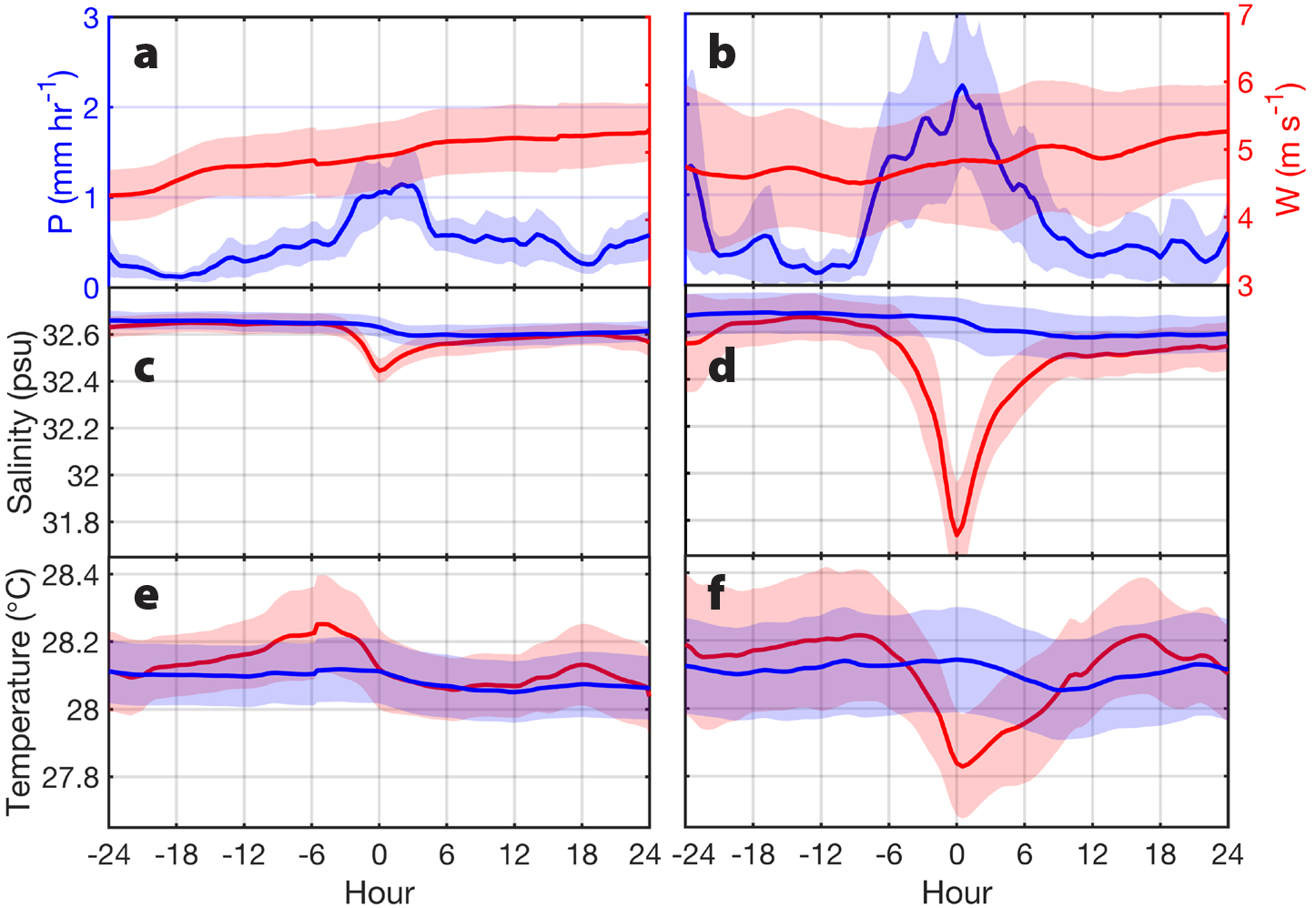
Figure 4. Composites for the periods of (a,c,e) moderate (0.05–0.5 psu) and (b,d,f) strong (>0.5 psu) salinity differences between 0.4 m and 5 m depths: (a–b) (blue) TRMM precipitation and (red) MERRA-2 wind speed; (c–d) salinity at (red) 0.4 m and (blue) at 5 m depths; (e–f) temperature at (red) 0.4 m and (blue) 5 m depths. Shading shows 2 standard errors. > High res figure

 

All significant rain events are characterized by a rapid (3–6 hours long) decrease of surface salinity and then a more gradual recovery after the precipitation reaches its maximum. The average decrease of salinity at 0.4 m depth is 0.21 ± 0.05 psu for −0.5 <∆S ≤ −0.05 and 0.93 ± 0.06 psu for −2.0 ≤ ∆S < −0.5. Salinity at 5 m depth also decreases by 0.07 ± 0.06 psu for −0.5 <∆S ≤ −0.05 psu and by 0.11 ± 0.07 psu for −2.0 ≤ ∆S < −0.5. Although the observed salinity reduction at 5 m depth during rainfall is significant, the difference in salinity reduction between the two ∆S intervals is not. As expected, there is a time lag between freshening at the surface and the associated salinity change at 5 m depth. On average, it takes about two to three hours for salinity at 5 m depth to respond to rapid freshening at the surface.

It is interesting to note that rain-​induced freshening is also associated with surface cooling, likely because freshwater brought by rainfall is usually colder than the seawater. In addition, winds tend to be stronger during rain events, which enhances evaporation and also contributes to surface cooling. The observed surface cooling during the peak of precipitation is −0.19 ± 0.17°C for weak and moderate surface freshening (−0.5 < ∆S ≤ −0.05) and −0.39 ± 0.13°C for strong freshening (−2.0 ≤ ∆S < −0.5). There is also a slight cooling at 5 m depth in both cases, but it is not statistically significant.

One of the interesting questions is how long the precipitation-induced salinity anomalies (rain puddles) persist before they dissipate. The advantage of using surface drifters over other types of measurements is that drifters provide quasi-Lagrangian observations by following currents and advection pathways at 15 m depth. If the vertical gradient of horizontal velocity between the surface and 15 m depth were small, the drifters would tend to move with salinity anomalies caused by patchy rain events. Thus, they would be able to trace rain puddles until they dissipate, providing estimates of their lifetimes. In reality, however, if there is vertical velocity shear, rain puddles can move differently than the water at 15 m depth. In this case, drifters will occasionally cross rain-induced salinity anomalies before they disappear, resulting in a low lifetime bias. Nevertheless, up to now these are the best observations of rain puddles in a Lagrangian sense, and our drifter observations provide the lower bounds for the lif­­­etime of rain-induced salinity anomalies. As follows from the composites in Figure 4, the duration of freshening is mostly limited by rain events, although it is necessary to remember a much larger auto-correlation of rain data compared to drifter records. The lifetime of rain-induced freshening (rain puddles) can span up to 24 hours, although the largest ∆S is observed over the period of a few hours, as previously reported (e.g., Boutin et al., 2016).

 

Relationship Between Temperature and Salinity Differences

Earlier deployment of identical dual-​sensor drifters in the evaporation-​dominated subtropical South Pacific in 2015 revealed a positive correlation between the temperature (∆T) and salinity (∆S) differences between the two measurement depths (Dong et al., 2017). Drifters deployed in the ITCZ during the SPURS-2 campaign exhibit a similar relationship (Figure 3a). Three regimes are evident: (1) surface salinification (∆S > 0) and warming (∆T > 0), (2) surface freshening (∆S < 0) and cooling (∆T < 0), and (3) surface freshening (∆S < 0) and warming (∆T > 0). The latter regime is apparently associated with occurrences of rainfall being warmer than the sea­water and/or with cases when solar heating warmed the surface of a salinity anomaly before it dissipated. We find that both are independent of the strength of a salinity anomaly. Despite the atmospheric forcing in all three regimes, the upper 5 m of the water column remained stably stratified, as illustrated by the density differences between 0.4 m and 5 m depth (Figure 3a).

The first two regimes (salinification and warming; freshening and cooling) to some extent exhibit a linear relationship between ∆T and ∆S. The correlation between ∆T and ∆S for the periods of surface salinification and warming is 0.65, while the correlation between ∆T and ∆S for the periods of surface freshening and cooling is 0.79. For the first regime, strong diurnal surface warming (∆T > 0) and evaporation, which usually happen during clear sky and low wind conditions, can make the surface water saltier than water at 5 m depth (∆S > 0; e.g., days 235–236 in Figure 1c and days 256, 273, 287 in Figure 2b,d). The linear regression analysis suggests that a 1°C temperature difference between 0.4 m and 5 m depth leads to an approximately 0.05 ± 0.02 psu difference in salinity, where the uncertainty is one standard deviation of the residuals (Figure 3b). This is exactly the same rate we obtained earlier in the subtropical South Pacific (Dong et al., 2017). The differences become larger at low wind speeds (generally less than 3 m s^–1), but generally stay below 0.1 psu, in agreement with an empirical model by Asher et al. (2014b).

For the second regime (freshening and cooling), if the salinity difference is regarded as an indicator of the amount of colder rainwater entering the ocean, then regressing ∆T on ∆S (predictor) yields surface cooling of about 0.4 ± 0.04°C per 1 psu surface freshening (Figure 3c). The scatter between ∆T and ∆S for the periods of surface freshening and cooling indicates that the large negative salinity differences of less than −0.5 psu most of the time occur at wind speeds below 6 m s^–1. Nevertheless, it is interesting to note that there is an isolated cluster of points with large negative ∆T and ∆S and wind speeds of about 7 m s^–1 (Figure 3c). This cluster is associated with strong rainfall that overcomes the enhanced wind-induced mixing and still generates large ∆S, while both rainwater and wind favor stronger negative ∆T. The observed dependence between ∆T and ∆S for the periods of freshening and cooling compares well to earlier studies (Reverdin et al., 2012; Bellinger et al., 2016).

 

Diurnal Cycles of Temperature and Salinity

Daytime warming and nighttime cooling cause the diurnal cycles of temperature and salinity in the drifter records. The diurnal cycle is particularly pronounced in temperature records at both measurement depths (e.g., Figure 2a). To analyze the properties of the diurnal signals, the drifter records were first subsampled at 10-minute intervals and then averaged to hourly. The daily averages at the two measurement depths were subtracted in order to remove day-to-day variability, and the record-averaged temperature and salinity were added back. Periods with ∆S < −0.2 psu, presumably corresponding to strong rain events, were masked, so that they did not influence the computation of the diurnal amplitude and phase. The diurnal cycle was then obtained by the least-squares fit of two harmonic functions with diurnal and semidiurnal frequencies. The amplitude and phase were computed as the half-range of the sum of these functions and the hour of the daily maximum, respectively.

During clear sky and low wind conditions, diurnal warming at the surface can substantially exceed (up to 2°C) the diurnal warming at 5 m depth (Figure 2a). The average amplitudes of the diurnal cycle of temperature are about 0.12°C at the surface and 0.05°C at 5 m depth (Figure 5a), very close to those observed earlier in the subtropical South Pacific (Dong et al., 2017). The daily maximum of temperature at the surface is observed at 14:30 solar time. Because it takes some time for the heat to reach deeper layers, the daily maximum at 5 m is observed at 16:30 solar time. The diurnal cycle of salinity is only well pronounced at the surface, reaching an amplitude of 4 × 10^–3 psu, which is just slightly above the accuracy of the conductivity sensor (±3 × 10^–3 psu) (Figure 5b). The small diurnal amplitude of the near-surface salinity confirms earlier observations in other regions with moorings (Cronin and McPhaden, 1999) and drifters (Reverdin et al., 2012; Dong et al., 2017). It is interesting to note that during nighttime cooling, the surface tends to be slightly (although statistically insignificantly) colder than the water at 5 m depth (no matter the potential or in situ temperature used; Figure 5a). However, the greater daily averaged salinity at 5 m depth compared to salinity at 0.4 m depth (Figure 5b) maintains stable density stratification at almost all times (Figure 3a).

 

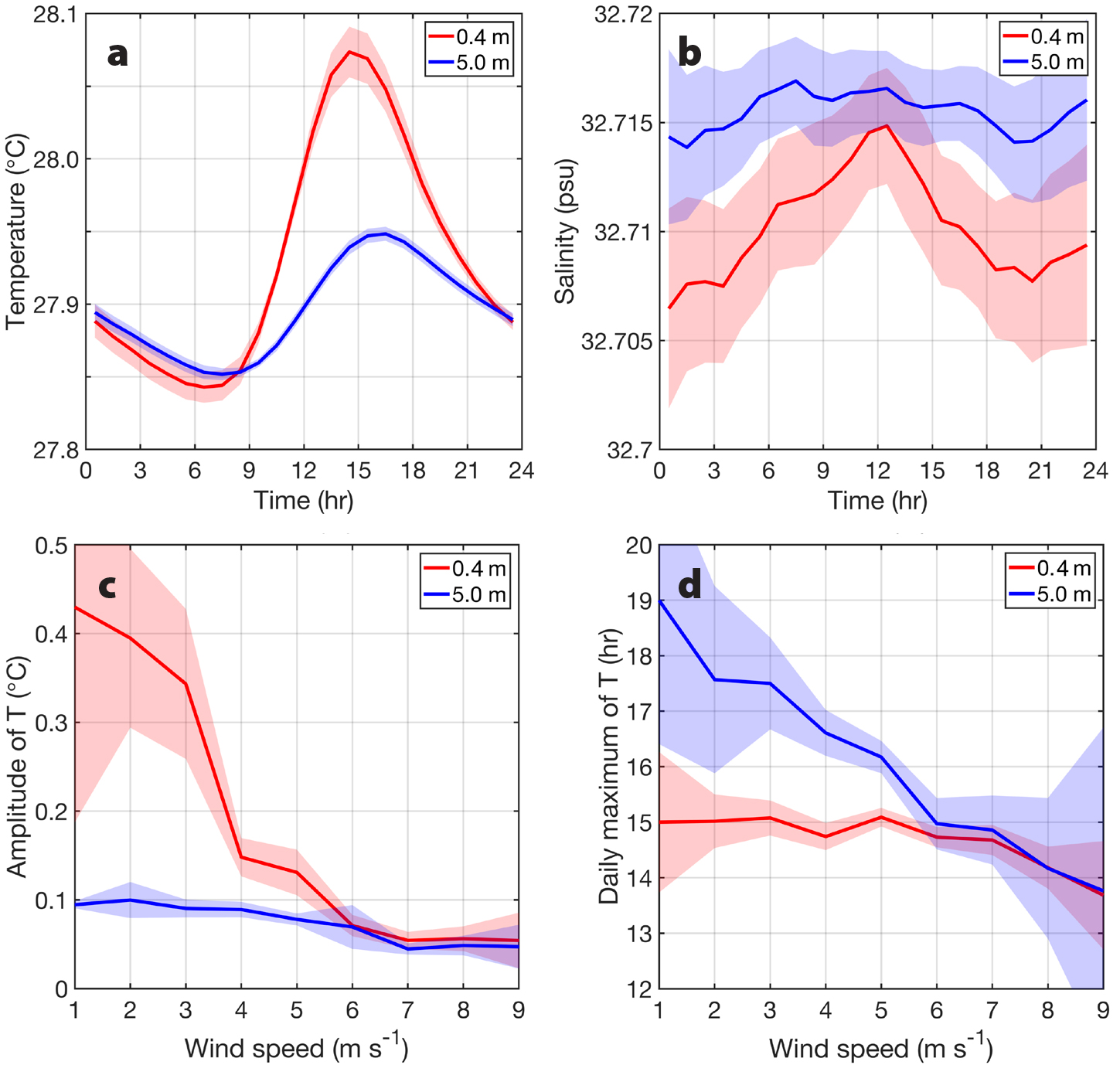
Figure 5. Diurnal cycles of (a) temperature and (b) salinity at (red) 0.4 m and (blue) 5 m depths. (c) Diurnal amplitude of temperature at (red) 0.4 m and (blue) 5 m depths in relation to wind speed. (d) The timing of daily maximum of temperature at (red) 0.4 m and (blue) 5 m depths in relation to wind speed. Shading shows 2 standard errors. > High res figure

 

The diurnal amplitude of temperature depends on the wind speed (Figure 5c). At the surface, it reduces by an order of magnitude, from around 0.4°C to 0.05°C, as the wind speed increases from 1 m s^–1 to 9 m s^–1. This is expected, because at low wind speeds, (1) the sky is either clear or partly cloudy, so that the diurnal warming is enhanced by direct solar heating, (2) there is less latent heat flux, and (3) weak mixing suppresses the downward turbulent heat flux in the upper water column. At 5 m depth and for the same range of wind speeds, the amplitude reduces more gradually from 0.1°C to 0.04°C. The uncertainty in the amplitude at the surface is very large at low wind speeds (±0.22°C at 1 m s^–1). This is partly because the amplitude is also a function of insolation, which can vary significantly depending on cloudiness. At stronger wind speeds, the sky is usually overcast, thus reducing the fluctuations of insolation. At wind speeds above 6 m s^–1, the diurnal amplitude at the surface is not statistically different from that at 5 m depth, meaning that the upper water column becomes well mixed. Wind has little impact on the timing of the daily temperature maximum at the surface, but it strongly influences it at 5 m depth (Figure 5d). Generally, temperature at the surface reaches its maximum between 14:00 and 15:00 solar time. At low wind speeds (0–3 m s^–1) when vertical mixing is weak, the diurnal temperature maximum at 5 m depth occurs two to four hours later. At wind speeds above 6 m s^–1, the times of the diurnal maxima at both depths are not statistically different from each other.

 

Comparison with Satellite Sea Surface Salinity

The mean ∆S measured by drifters in the ITCZ (Table 1) is more than an order of magnitude smaller than the differences between the satellite SSS and the uppermost measurements of salinity by Argo floats (±0.5 psu). This supports a conclusion by Dong et al. (2017) that the differences between the satellite skin measurements and in situ data are not due to the differences in measurement depths. To validate the satellite SSS with drifter measurements at 0.4 m depth, the drifter records were linearly interpolated onto concurrent 10-day averaged debiased Release-5 SSS maps from SMOS at three resolutions (25, 50, and 100 km) and on daily (eight-day running mean) Version-4 SSS maps from SMAP at a resolution of about 60 km (both SMOS and SMAP are Level 3 data). The satellite-​derived SSS records for the first 10 days of drifter #145738 measurements are shown in Figure 1c, and the root-mean-square (RMS) differences between salinities at 0.4 m depth measured by all six drifters and SSS are presented in Table 2.

 

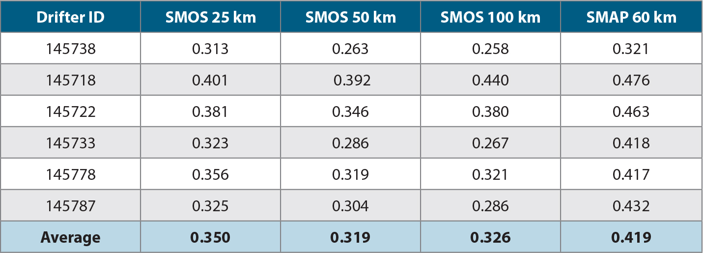
Table 2. Root-mean-square differences (psu) between the drifter salinity measurements at the surface (S0.4) and the collocated satellite-derived SSS from SMOS and SMAP missions at different spatial resolutions. The average is weighted by the number of valid measurements by each drifter. > High res table

 

The RMS differences demonstrate that errors in satellite retrievals are rather large (0.3–0.4 psu) and similar to the differences between the satellite SSS and Argo salinity at 5 m depth. The RMS differences in Table 2 are greater than the RMS differences between the two drifter measurement depths (~0.1 psu). While the satellite SSS data more or less adequately resolve the spatial trends in salinity related to mesoscale features in the ocean, the satellite’s repeat cycle and the size of the footprint do not allow full resolution of the shorter and smaller scale variability related to the diurnal cycle and rainfall events (Figure 1c). In addition, satellite SSS is still subject to biases and temporal inconsistencies between the consecutive maps, which are seen as step-like changes of SSS from one map to another in Figure 1c.

 

Conclusions

The deployment of dual-sensor Lagrang-ian drifters during the SPURS-2 field campaign in the precipitation-dominated ITCZ in the eastern equatorial Pacific revealed details in the near-surface salinity and temperature structures that are difficult or impossible to observe with other platforms. Measuring salinity and temperature nearly at the surface (0.4 m depth) and at the standard uppermost depth of in situ observations (5 m) provides a point of reference for investigating the upper 5 m stratification and validating the satellite retrievals.

Analysis of the upper 5 m stratification reveals dependencies of temperature and salinity gradients on each other, and on wind speed and precipitation. The observed temperature and salinity differences between 0.4 m and 5 m depths are significantly correlated with each other for the following two regimes. (1) On one hand, strong diurnal heating of the ocean’s surface enhances evaporation and leads to stable temperature and unstable salinity stratification. (2) On the other hand, because rain­water is usually colder than the ocean’s surface, freshening during rainfall events is usually accompanied by a sizable surface cooling. Nevertheless, the mean temperature difference between the two measurement depths remains positive, mostly due to the well-pronounced diurnal cycle at the surface. Despite the occurrences of unstable salinity stratification, the density stratification remained stable throughout the experiment except in a few instances.

In precipitation-dominated regions, surface freshening during strong rainfall and weak winds can result in salinity differences between the two measurement depths of up to 2 psu. Winds stronger than about 6 m s^–1 induce strong vertical mixing that inhibits the formation of the upper 5 m salinity gradient regardless of the strength of precipitation. Most of the largest salinity gradients are observed with wind speeds below 3 m s^–1. The evolution of salinity measurements at 0.4 m and 5 m depths suggests that significant rain events are characterized by the rapid decrease of the surface salinity and then by a more gradual recovery period. The salinity at 5 m depth responds to this freshening with a delay of two to three hours. A unique aspect of using Lagrangian drifters to measure rain-induced salinity anomalies is that they provide estimates of the lifetimes of rain puddles, which we estimate can last at least 24 hours.

The half-hourly drifter data exhibit the diurnal cycle of temperature at both 0.4 m and 5 m depths, and the diurnal cycle of salinity at 0.4 m. Stronger winds favor vertical mixing and, thus, reduce the diurnal amplitude of temperature, in particular at the surface. While the reduction of the diurnal amplitude at 5 m with increasing wind speeds is almost an order of magnitude smaller than at the surface, the time of the daily maximum at 5 m depth is much more strongly influenced by wind speed. For low wind speeds (< 5 m s^–1), the daily temperature maximum at 5 m occurs one to four hours later than at the surface. With stronger winds (> 6 m s^–1), the diurnal amplitudes and phases of temperature at both depths do not change significantly, and they are not statistically different from each other, meaning that the upper 5 m has become well mixed.

The first three months of drifter measurements show that the mean salinity difference between 0.4 m and 5 m depths is negative, but very small (−0.016 ± 0.094 psu, where the uncertainty is one standard deviation). However, a comparison of drifter measurements at 0.4 m depth with satellite SSS products shows much larger (more than an order of magnitude) discrepancies. This means that the differences that have been observed between satellite SSS and near-surface (generally at 5 m depth) in situ salinity measurements generally are not related to the difference in the measurement depths, but are rather due to errors in SSS retrievals, unresolved subfootprint processes (e.g., rainfall, wind gusts, variations of insolation, submesoscale fronts), or filtering and interpolation methods.

Volkov, D.L., S. Dong, G.R. Foltz, G. Goni, and R. Lumpkin. 2019. Observations of near-​surface salinity and temperature structure with dual-​sensor Lagrangian drifters during SPURS-2. Oceanography 32(2):66–75, https://doi.org/10.5670/oceanog.2019.214.

Asher, W.E., A.T. Jessup, R. Branch, and D. Clark. 2014a. Observations of rain-induced near-​surface salinity anomalies. Journal of Geophysical Research 119:5,483–5,500, https://doi.org/​10.1002/​2014JC009954.
1. Asher, W.E., A.T. Jessup, and D. Clark. 2014b. Stable near-surface ocean salinity stratifications due to evaporation observed during STRASSE. Journal of Geophysical Research 119:3,219–3,233, https://doi.org/​10.1002/2014JC009808.
2. Bellinger, H., K. Drushka, W. Asher, G. Reverdin, M. Katsumata, and M. Watanabe. 2017. Extension of the prognostic model of sea surface temperature to rain-induced cool and fresh lenses. Journal of Geophysical Research 122:484–507, https://doi.org/​10.1002/2016JC012429.
3. Boutin, J., N. Martin, G. Reverdin, X. Yin, and F. Gaillard. 2013. Sea surface freshening inferred from SMOS and Argo salinity: Impact of rain. Ocean Science 9:183–192, https://doi.org/10.5194/os-9-183-2013.
4. Boutin, J., Y. Chao, W.E. Asher, T. Delacroix, R. Drucker, K. Drushka, N. Kolodziejczyk, T. Lee, N. Reul, G. Reverdin, and others. 2016. Satellite and in situ salinity: Understanding near-surface stratification and subfootprint variability. Bulletin of the American Meteorological Society 97:1,391–1,407, https://doi.org/10.1175/BAMS-D-15-00032.1.
5. Cronin, M.F., and M.J. McPhaden. 1999. Diurnal cycle of rainfall and surface salinity in the Western Pacific Warm Pool. Geophysical Research Letters 26(23):3,465–3,468, https://doi.org/​10.1029/1999GL010504.
6. Dong, S., D. Volkov, G. Goni, R. Lumpkin, and G.R. Foltz. 2017. Near-surface salinity and temperature structure observed with dual-​sensor drifters in the subtropical South Pacific. Journal of Geophysical Research 122, https://doi.org/​10.1002/​2017JC012894.
7. Drushka, K., W.E. Asher, B. Ward, and K. Walesby. 2016. Understanding the formation and evolution of rain-formed fresh lenses at the ocean surface. Journal of Geophysical Research 121:2,673–2,689, https://doi.org/10.1002/2015JC011527.
8. EUMETSAT SAF on Ocean and Sea Ice. 2016. ASCAT L2 12.5 km winds data record release 1-Metop. OSI SAF, https://doi.org/10.15770/EUM_SAF_OSI_0007.
9. Fore, A.G., S.H. Yueh, W. Tang, B. Stiles, and A.K. Hayashi. 2016. Combined active/passive retrievals of ocean vector wind and sea surface salinity with SMAP. IEEE Transactions on Geoscience and Remote Sensing 54:7,396–7,404, https://doi.org/10.1109/TGRS.2016.2601486.
10. GMAO (Global Modeling and Assimilation Office). 2015. MERRA-2 inst1_2d_asm_Nx: 2d, 1-Hourly, Instantaneous, Single-Level, Assimilation, Single-Level Diagnostics V5.12.4. Greenbelt, MD, USA, Goddard Earth Sciences Data and Information Services Center (GES DISC), https://doi.org/​10.5067/​3Z173KIE2TPD.
11. Grodsky, S.A., J.A. Carton, and H. Liu. 2008. Comparison of bulk sea surface and mixed layer temperatures. Journal of Geophysical Research 113, C10026, https://doi.org/10.1029/2008JC004871.
12. Hodges, B.A., and D.M. Fratantoni. 2014. AUV observations of the diurnal surface layer in the North Atlantic salinity maximum. Journal of Physical Oceanography 44:1,595–1,604, https://doi.org/​10.1175/​JPO-D-13-0140.1.
13. Huffman, G.J., R.F. Adler, D.T. Bolvin, and E.J. Nelkin. 2010. The TRMM Multi-satellite Precipitation Analysis (TMPA). Chapter 1 in Satellite Rainfall Applications for Surface Hydrology. https://doi.org/​10.1007/978-90-481-2915-7.
14. Kerr, Y.H., P. Waldteufel, J.-P. Wigneron, S. Delwart, F. Cabot, J. Boutin, M.-J. Escorihuela, J. Font, N. Reul, C. Gruhier, and others. 2010. The SMOS mission: New tool for monitoring key elements of the global water cycle. Proceedings of the IEEE 98:666–687, https://doi.org/10.1109/JPROC.2010.2043032.
15. Lagerloef, G., F.R. Colomb, D. Le Vine, F. Wentz, S. Yueh, C. Ruf, J. Lilly, J. Gunn, Y. Chao, A. deCharon, G. Feldman, and C. Swift. 2008. The Aquarius/SAC-D mission: Designed to meet the salinity remote-sensing challenge. Oceanography 21(1):68–81, https://doi.org/10.5670/oceanog.2008.68.
16. Lindstrom, E.J., A.Y. Shcherbina, L. Rainville, J.T. Farrar, L.R. Centurioni, S. Dong, E.A. D’Asaro, C. Eriksen, D.M. Fratantoni, B.A. Hodges, and others. 2017. Autonomous multi-platform observations during the Salinity Processes in the Upper-ocean Regional Study. Oceanography 30(2):38–48, https://doi.org/​10.5670/​oceanog.2017.218.
17. Reverdin, G., S. Morisset, J. Boutin, and N. Martin. 2012. Rain-induced variability of near sea-​surface T and S from drifter data. Journal of Geophysical Research 117, C02032, https://doi.org/​10.1029/​2011JC007549.
18. Rhein, M., S.R. Rintoul, S. Aoki, E. Campos, D. Chambers, R.A. Feely, S. Gulev, G.C. Johnson, S.A. Josey, A. Kostianoy, and others. 2013. Observations: Ocean. Pp. 255–315 in Climate Change 2013: The Physical Science Basis. Contributions of Working Group I to the Fifth Assessment Report of the Intergovernmental Panel on Climate Change. T.F. Stockeret D. Qin, G.-K. Plattner, M. Tignor, S.K. Allen, J. Boschung, A. Nauels, Y. Xia, V. Bex, and P.M. Midgley, eds, Cambridge University Press, Cambridge, United Kingdom and New York, NY, USA.
19. Schanze, J.J., G. Lagerloef, R.W. Schmitt, and B.A. Hodges. 2014. Snakes on a ship: Surface salinity observations during SPURS. Extended Abstracts, 2014 Ocean Sciences Meeting, Honolulu, HI, ASLO-AGU, 073.
20. Supply, A., J. Boutin, J.-L. Vergely, N. Martin, A. Hasson, G. Reverdin, C. Mallet, and N. Viltard. 2017. Precipitation estimates from SMOS sea-​surface salinity. Quarterly Journal of the Royal Meteorological Society 144:103–119, https://doi.org/​10.1002/​qj.3110.
21. TRMM (Tropical Rainfall Measuring Mission). 2011. TRMM (TMPA) Rainfall Estimate L3 3 hour 0.25 degree x 0.25 degree V7. Greenbelt, MD, Goddard Earth Sciences Data and Information Services Center (GES DISC), https://doi.org/10.5067/TRMM/TMPA/3H/7.

This is an open access article made available under the terms of the Creative Commons Attribution 4.0 International License (https://creativecommons.org/licenses/by/4.0/), which permits use, sharing, adaptation, distribution, and reproduction in any medium or format as long as users cite the materials appropriately, provide a link to the Creative Commons license, and indicate the changes that were made to the original content. Images, animations, videos, or other third-party material used in articles are included in the Creative Commons license unless indicated otherwise in a credit line to the material. If the material is not included in the article’s Creative Commons license, users will need to obtain permission directly from the license holder to reproduce the material.