Ocean biogeochemical models have become critical tools for interpreting trace element and isotope (TEI) distributions observed during the GEOTRACES program and understanding their driving processes. Models stimulate new research questions that cannot be addressed with observations alone, for instance, concerning processes that occur over vast spatial scales and linkages between TEIs and other elemental cycles. A spectrum of modeling approaches has been applied to date, including (1) fully prognostic models that couple TEIs to broader biogeochemical frameworks, (2) simpler element-specific mechanistic models that allow for assimilation of observations, and (3) machine learning models that have no mechanistic underpinning but allow for skillful extrapolation of sparse data. Here, we evaluate the strengths and weaknesses of these approaches and review three sets of novel insights they have facilitated. First, models have advanced our understanding of global-scale micronutrient distributions, and their deviations from macronutrients, in terms of a “ventilation-regeneration-scavenging” balance. Second, models have yielded global-scale estimates of TEI inputs to and losses from the ocean, revealing, for instance, a rapid iron (Fe) cycle with an oceanic residence time on the order of decades. Third, models have identified novel links among various TEI cycling processes and the global ocean carbon cycle, such as tracing the supply of hydrothermally sourced Fe to iron-starved microbial communities in the Southern Ocean. We foresee additional important roles for modeling work in the next stages of trace element research, including synthesizing understanding from the GEOTRACES program in the form of TEI state estimates, and projecting the responses of TEI cycles to global climate change.

Model-simulated aluminum distribution along the GEOTRACES GA02 section in the West Atlantic Ocean. The black labeled arrows represent ocean circulation pathways. Modified from Xu and Weber (2021). > High res figure

Background and Motivation

The overall mission of the GEOTRACES program is “to identify processes and quantify fluxes that control the distributions of key trace elements and isotopes (TEIs) in the ocean, and to establish the sensitivity of these distributions to changing environmental conditions” (GEOTRACES Planning Group, 2006). Addressing these challenges requires the community to move beyond direct quantification of concentrations to explore key fluxes and cycling mechanisms. While this has proceeded via observational efforts as part of GEOTRACES section and process study voyages, numerical models that resolve critical processes and properties are also playing a growing role and are now considered an integral part of the GEOTRACES toolkit.

A wide range of modeling frameworks with varying complexity have been applied to interpret GEOTRACES observations. Because even the most complex models remain incomplete, they represent simplified views of the dominant biogeochemical processes governing TEI cycling as they are embedded within ocean circulation models that are often too coarse to accurately capture the scales of TEI fluxes across ocean boundaries and within the water column. Numerous papers have been written enumerating the shortcomings and biases of TEI models and their inability to reproduce the finer details of GEOTRACES data (e.g., Tagliabue et al., 2016; Eisenring et al., 2022). Nevertheless, the application of these imperfect models has often advanced our understanding of TEI distributions and cycling, yielding myriad new insights that could never have been gleaned from observations alone. Specifically, models have facilitated (1) extrapolation of sparse TEI observations, (2) testing of hypotheses regarding controlling mechanisms, and (3) upscaling and assessment of TEI impacts on the carbon cycle and its response to climate change. In this way, the field of TEI modeling has closely conformed to British statistician George E.P. Box’s classic mantra that “All models are wrong, but some are useful.”

The objective of this manuscript is not to provide an exhaustive review of all TEI modeling studies that have leveraged GEOTRACES data. Instead, our goals are threefold: (1) to provide a concise description of the general categories of models that are commonly used in this field and an assessment of their strengths and weaknesses; (2) to highlight with examples some key successes, where models have provided novel insight into the cycling of TEIs and made critical contributions toward the GEOTRACES mission; and (3) to outline a set of outstanding challenges to and opportunities for developing this model-data nexus further in the coming years.

 

Categories of TEI Models

The wide range of modeling approaches that have contributed to our understanding of TEI cycling vary in their complexity, resolution, predictive capabilities, and how they leverage observations. Here, we recognize three broad categories of models: (1) fully prognostic biogeochemical models, (2) element-​specific transport matrix models, and (3) machine learning and diagnostic models. The first two categories are both mechanistic in that they simulate trace element cycles inside ocean circulation models using mathematical functions that represent TEI sources, sinks, and internal cycling processes. They differ, however, in scope and how extensively they incorporate GEOTRACES observations in order to refine the mechanistic framework. The third category is not underpinned by a mechanistic understanding of TEI cycling but instead leverages observations only in a statistical sense. The three categories thus define a spectrum between prognostic and diagnostic modeling philosophies, with the former predicting the state of a system (here, the distribution of a TEI) based on mechanistic process information and the latter inferring process information from a known system state. Below, we review the distinguishing features of each category and their unique strengths and weaknesses.

 

Fully Prognostic Biogeochemical Models

In this type of model, the mechanistic representation of trace element cycling is coupled to an existing biogeochemical framework that resolves multiple nutrient cycles, planktonic ecosystems, formation and degradation of particulate and dissolved organic matter, oxygen, and inorganic carbon chemistry (Figure 1a). These marine biogeochemical models are either run independently (at the global scale, or at high resolution regional scales) or further coupled with atmospheric and terrestrial modeling components to comprise an Earth system model that can be used for climate projection (Seferian et al., 2020). In contrast to the other two modeling categories we define, there is no explicit incorporation of GEOTRACES observations to constrain the model. Instead, a large-scale TEI distribution emerges solely as a prediction of the source, sink, and cycling parameterizations adopted (hence, “fully prognostic”), although model-data comparison is employed for validation, to inform the inclusion of key processes, and to guide parameter selection.

Due to its critical role in limiting primary production, the iron (Fe) cycle is now represented in almost all biogeochemical models incorporated in Earth system models, although the level of detail and predictive skill of these models varies widely (Tagliabue et al., 2016). Currently, additional micronutrients like cobalt (Co), copper (Cu), manganese (Mn), and zinc (Zn) are being added to prognostic models (Figure 1a), with the end goal of resolving their biological roles in co-limiting productivity and shaping the microbial ecosystem (Richon and Tagliabue, 2019; Tagliabue et al., 2018; Hawco et al., 2022). Efforts have also been made to couple the cycling of non-​bioactive elements, such as Al, Pa/Th, and Nd, to fully prognostic biogeochemical models (Arsouze et al., 2009; van Hulten et al., 2013, 2014, 2018).

 

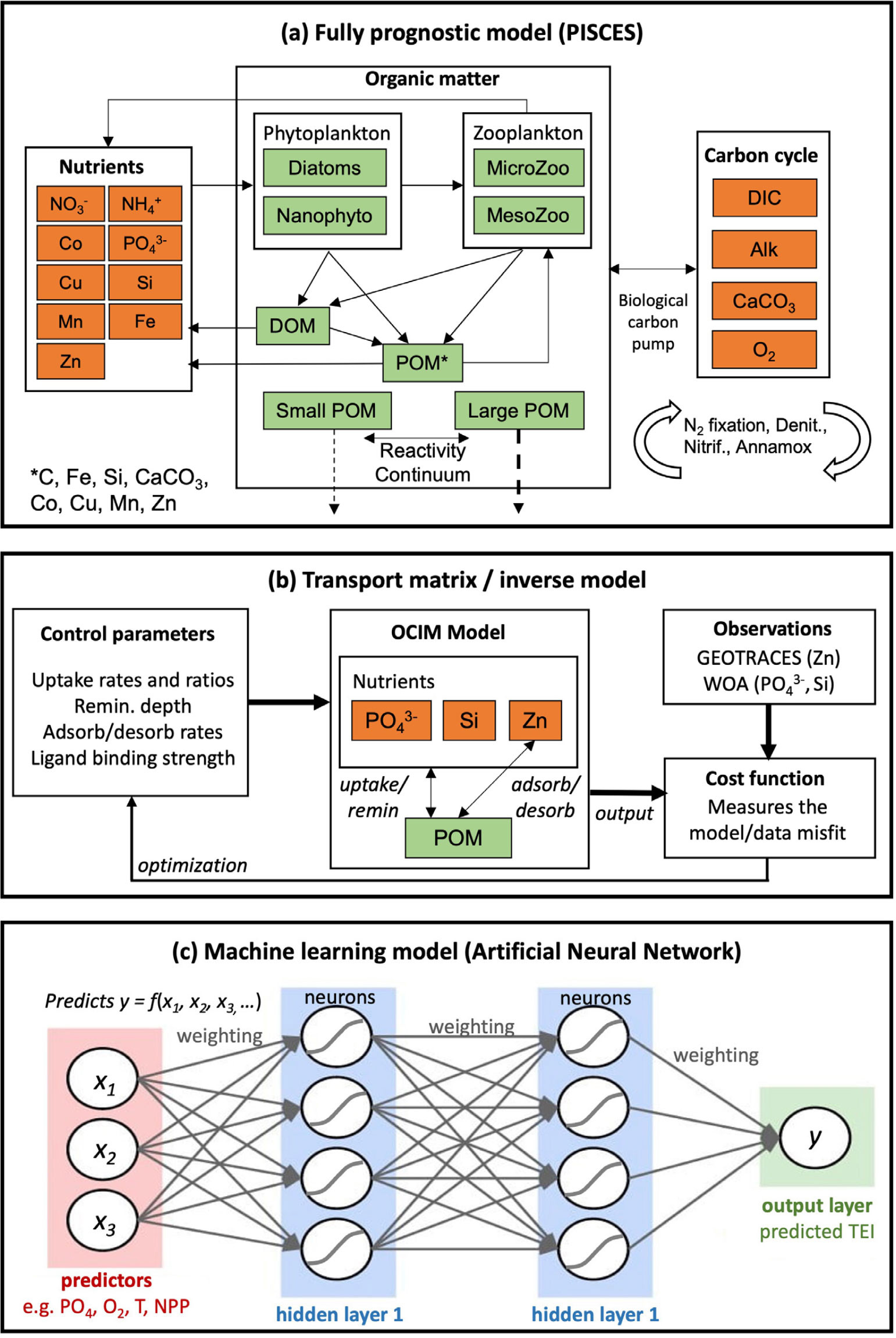
FIGURE 1. Schematic illustrations of three trace element and isotope (TEI) modeling categories. (a) In the fully prognostic PISCES model (Tagliabue et al., 2023a), TEIs are linked to a broader biogeochemical framework. (b) In a transport matrix inverse model, parameters are optimized using GEOTRACES data to constrain the oceanic Zn cycle (Weber et al., 2018). Orange and green boxes in (a) and (b) represent inorganic and organic tracers predicted by the models that can be compared to observations. (c) In an artificial neural network model, a TEI is predicted statistically as a function of hydrographic and biogeochemical predictor variables. > High res figure

 

The primary strengths of prognostic biogeochemical models are that they link TEIs to the global carbon cycle and climate system (see section on Connecting Trace Metals to the Global Carbon Cycle) and are able to predict TEI cycle responses to environmental change, including potential TEI-climate feedback loops (Moore et al., 2018). They also explicitly resolve multiple processes spanning phytoplankton uptake, zooplankton recycling, particle dynamics, and abiotic TEI input and removal pathways. Their primary limitation is their computational cost—because each simulation requires days to weeks of supercomputer time, these models are not efficient tools for exploratory science and extensive hypothesis testing. While this limitation also prevents direct incorporation of GEOTRACES observations, prognostic models have made extensive use of hypotheses emerging from GEOTRACES observations and have been employed to assess multiple processes emerging from the external input and internal cycling of TEIs (e.g., Resing et al., 2015; Tagliabue et al., 2023a).

 

Element-Specific Transport Matrix Models

This category comprises mechanistic models that are specifically designed to explore the cycling of a single TEI, uncoupled from a broader biogeochemical framework (Figure 1b). The TEI of interest is often coupled to fluxes of one or two other nutrient tracers (e.g., phosphate, silicic acid) in order to resolve net biological cycling, rather than linking to a full planktonic ecosystem (John et al., 2019). Other biogeochemical flux parameterizations are similar (albeit simpler) to those used in fully prognostic models, with observed properties often standing in for model-predicted properties—for instance, anoxic processes may be linked to observed, rather than predicted, oxygen fields (e.g., Weber et al., 2018). The circulation of TEIs is often represented using the Transport Matrix Method—​a highly efficient method for directly predicting steady-state tracer distributions (Primeau, 2005; Khatiwala, 2007). Recently, the Ocean Circulation Inverse Model (DeVries and Holzer, 2019) has been widely adopted for this purpose, because it incorporates water mass and ventilation tracer data to ensure faithful representation of the large-scale global circulation in the ocean interior.

The strengths and limitations of these models are largely opposite to the previous category. They are highly computationally efficient (each simulation takes seconds to minutes), facilitating broad exploration, hypothesis testing, and assimilation of GEOTRACES data to “optimize” the model structure and parameters (i.e., seeking the formulations and parameter values that bring the predicted TEI distribution into best agreement with observations in an objective manner; Figure 1b). In this way, they are often used as “inverse models” that extract estimates of TEI sources, sinks, and internal cycling processes that are consistent with observed distributions. Inverse models can therefore be thought of as an intermediate on the spectrum between prognostic and diagnostic modeling philosophies, combining the mechanistic underpinning of the former with the observational underpinning of the latter. As for their limitations, these models lack temporal resolution (generally only predicting steady-state annual-mean TEI distributions), neglect complex biological processes (e.g., those associated with phytoplankton uptake or zooplankton recycling), cannot be used for future predictions, and do not resolve complex interactions between TEIs and other elemental cycles. Over the last decade, transport matrix models have been successfully applied to understand the large-scale distributions and oceanic budgets of a suite of TEIs (see later section on Understanding Fundamental Controls on Large-Scale Trace Element Distributions), including zinc (Vance et al., 2017; Weber et al., 2018), nickel (John et al., 2022), copper (Liang et al., 2023), iron (Pasquier and Holzer, 2018; Roshan et al., 2020), and aluminum (Xu and Weber, 2021).

 

Machine Learning and Diagnostic Models

Machine learning has been widely adopted in ocean biogeochemistry as a gap-filling tool to generate continuous spatial distribution estimates (“climatologies”) from sparse datasets, including those for greenhouse gases (Weber et al., 2019; Yang et al., 2020), organic matter (Roshan and DeVries, 2017), and more recently also TEIs (Roshan et al., 2018; Huang et al., 2022). Many of these applications have relied on artificial neural network (ANN) models, which can be thought of as sophisticated statistical models that are trained to predict a “target” variable (e.g., a TEI) through its relationship to a set of “predictor” variables—​hydrographic and biogeochemical properties such as temperature, salinity, nutrients, oxygen, and net primary production (Figure 1c). The statistical model is then applied to continuous gridded distributions of those predictors to generate a gridded estimate of the TEI distribution. Compared to more familiar statistical models (e.g., multiple linear regression), ANNs are structurally complex, comprising “hidden layers” of neurons in which each neuron is a nonlinear function of one or more inputs (predictor variables or the output of previous neurons), and neuron outputs eventually combine into a prediction of the TEI (Figure 1c). They are therefore often described as “black boxes,” in which the contribution of each input variable to the prediction is difficult to discern.

The primary strength of machine learning models is that, of all categories reviewed here, they make the most direct use of GEOTRACES observations in their TEI distribution predictions, and (by design) they reproduce those observations more accurately than the mechanistic models covered in the previous sections. However, their lack of mechanistic basis is the main weakness of machine learning models—they predict TEI distributions without providing any information about the processes underlying that distribution. To partially offset this weakness, a diagnostic modeling approach has been adopted, in which the TEI distributions predicted by machine learning models are combined with ocean circulation models to infer the patterns and rates of biogeochemical fluxes that are required to balance physical transport and mixing (e.g., Roshan et al., 2018). However, this method only provides a crude estimate of the net sources-minus-sinks, which cannot be separated into individual process rates or linked to environmental drivers.

 

Key Modeling Insights

Understanding Fundamental Controls on Large-Scale Trace Element Distributions

Since before the GEOTRACES era, ocean TEI distributions have been interpreted using the “preformed versus remineralized” component framework first developed to understand macronutrient distributions (Broecker et al., 1985). Here, observed subsurface tracer concentrations are defined as the sum of a preformed component carried by water masses from the ocean surface and a remineralized component that accumulates from organic matter decomposition (Ito and Follows, 2005). A classic application of this framework sought to explain the “kinked” (i.e., nonlinear) global cadmium (Cd) versus phosphate (PO₄) relationship in terms of preformed Cd depletion in intermediate waters and deep accumulation of remineralized Cd (de Baar et al., 1994). Over the last 15 years, ocean biogeochemical models have proved to be invaluable tools for interpreting the TEI distributions revealed by the GEOTRACES sections. Numerical models resolve preformed TEI distributions more realistically than traditional end-​member-​mixing calculations and can be used to test hypothesized biogeochemical mechanisms that modify TEI distributions in the ocean interior. For particle-reactive TEIs, the component framework has been expanded to consider a “ventilation-​remineralization-​scavenging” balance (Tagliabue et al., 2014, 2017; Weber et al., 2018), and models have elucidated the role of scavenging in stripping preformed and remineralized TEIs from subsurface waters or redistributing them over depth.

The most recent update to our understanding of the global Cd/PO₄ relationship has emerged from a machine-​learning and diagnostic-​modeling approach (Roshan and DeVries, 2021), which demonstrated that differences between the global Cd and PO₄ distributions can almost exclusively be traced to their preformed components. This is driven by extreme plasticity in Cd uptake during organic matter formation, with Cd:P uptake ratios reaching a global maximum in the Southern Ocean. Cd therefore becomes depleted in Antarctic Intermediate Water (AAIW), which propagates through the low latitudes at 1,000–2,000 m depth, and enriched in the ocean’s deep overturning cell. There is evidence for additional decoupling between Cd and PO₄ due to slightly deeper remineralization of the former, although this appears to work counter to the preformed decoupling by adding Cd back to Cd-deficient intermediate waters, slightly “unkinking” the global relationship (Roshan and DeVries, 2021).

A recent series of modeling studies, constrained by GEOTRACES section data, have demystified the paradoxical oceanic distribution of the important algal micronutrient zinc (Zn). Zn exhibits a much deeper concentration maximum than macronutrients and closely correlates with Si (Bruland et al., 1978), even though very little cellular Zn is incorporated alongside Si into diatom frustules (Ellwood and Hunter, 2000) and the vast majority is co-located with N and P in soft tissue (Twining and Baines, 2013). Biogeochemical models have revealed that the Si-like Zn distribution is largely controlled by efficient biological drawdown in the Southern Ocean surface, which strips Zn from AAIW and traps it in Antarctic Bottom Water (Vance et al., 2017; Weber et al., 2018), much like Si (Holzer et al., 2014). The stoichiometric signature of Southern Ocean water masses therefore imprints a Zn deficit (relative to PO₄) throughout the global upper ocean and a Zn excess throughout the deep ocean (Figure 2a,b). However, models in which vertical biogeochemical cycling of Zn mirrors PO₄ tend to underpredict Zn in the deep North Pacific and overpredict Zn in intermediate waters (Weber et al., 2018). These discrepancies can be resolved by weak reversible scavenging of Zn onto sinking particles, in which <1% of the oceanic Zn inventory exists in an adsorbed phase (Weber et al., 2018)—a conclusion that is also supported by a machine learning and diagnostic modeling approach (Roshan et al., 2018). Reversible scavenging strengthens the Zn deficit in the upper ocean (Figure 2c) by transferring Zn from intermediate to deep water masses (Figure 2d). Scavenging removal and subsequent redistribution of Zn also provides a mechanism for explaining the isotopic depletion of Zn in the upper ocean by removing isotopically heavy Zn and depositing it at mid-depths after the carrier particles remineralize (Sieber et al., 2023).

 

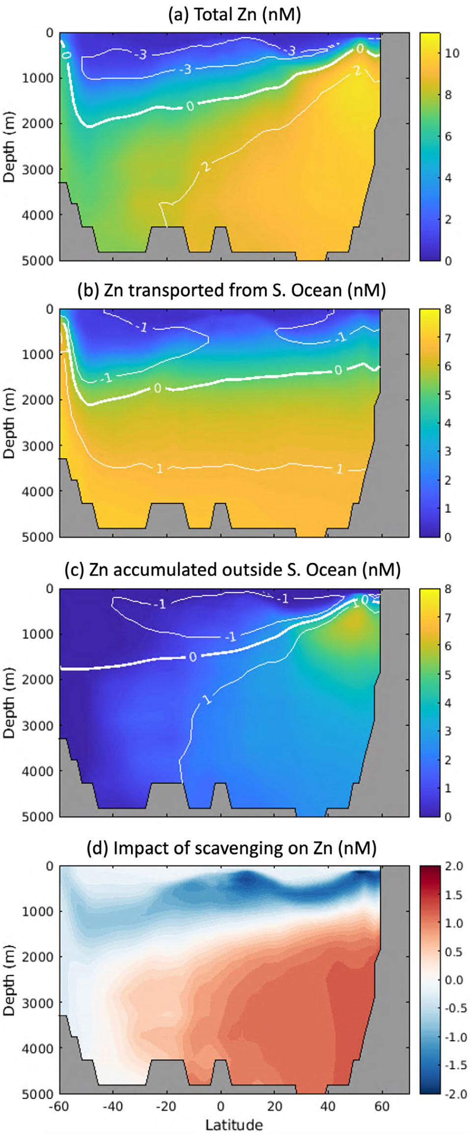
FIGURE 2. Model-based interpretation of global Zn distribution. (a) Predicted dissolved Zn distribution along 150°W in the Pacific Ocean, which compares well with observations from the GP15 cruise (Sieber et al., 2023). (b) Component of the Zn distribution that is transported from the Southern Ocean in Antarctic Intermediate Water (AAIW) and Antarctic Bottom Water (AABW) masses. (c) Component of Zn distribution that accumulates along transport pathways after water masses leave the Southern Ocean, due to vertical biogeochemical cycling. In (a)–(c), the white contours illustrate the Zn deficit or excess relative to PO4 defined as [Zn] – RZn:P[PO4], where RZn:P is the mean ocean Zn/PO4 ratio of 2.5 mmol mol–1. Together, (a)–(c) illustrate that the global Zn deficit in intermediate waters and excess in deep waters (a) is partially transported from the Southern Ocean (b), and partially generated by vertical cycling processes outside the Southern Ocean (c). (d) The impact of scavenging on Zn distribution is quantified here as the difference between models with and without scavenging enabled. Figures adapted from Weber et al. (2018) and Sieber et al. (2023). > High res figure

 

Unlike Zn and Cd, the micronutrient nickel (Ni) is found in excess relative to macronutrients throughout the surface ocean. According to recent modeling work (John et al., 2022), this is explained by slow Ni uptake in productive upwelling regions and restriction of Ni uptake by macronutrient limitation in subtropical gyres (i.e., low stoichiometric plasticity). While this surface distribution allows unutilized Ni to subduct in intermediate waters and would produce a similar preformed distribution to PO₄ and NO₃, observed Ni actually reaches a deeper maximum. Transport matrix modeling again demonstrates that this phenomenon is well explained by weak scavenging and desorption of Ni, which redistributes it over depth and drives a large-scale decoupling of its distribution from PO₄ and NO₃ (John et al., 2022).

The modeling studies outlined above reveal a dominant role for ventilation (i.e., the preformed component) in explaining the oceanic distributions of TEIs with long residence times. In contrast, elements with short residence times (like Fe) are removed too quickly to propagate with water masses far into the ocean interior. In this case, a balance between remineralization, scavenging, and boundary inputs governs TEI distribution, and the relative rates of those processes can be gleaned with models from GEOTRACES section data. Unlike macronutrients, dissolved Fe (DFe) does not increase systematically in the deep ocean with water mass age, reflecting a close compensation between scavenging and remineralization (Tagliabue et al., 2014, 2019), and instead often exhibits a mid-depth maximum between 200 m and 1,000 m (e.g., Figure 3a). Biogeochemical modeling attributes many of these features to the uptake and scavenging of dust-sourced Fe in the surface, followed by Fe remineralization and the release of scavenged Fe in the shallow subsurface (Pham and Ito, 2018). Beneath the mid-depth maximum, Fe remineralization is too slow, relative to scavenging, to allow significant remineralized Fe accumulation (Pham and Ito, 2018). In fact, model trajectory calculations indicate that the majority of remineralized Fe will be scavenged before re-emerging at the ocean’s surface and that most Fe supplied in upwelling water to the ocean surface is not the product of organic matter remineralization (Pasquier and Holzer, 2018).

 

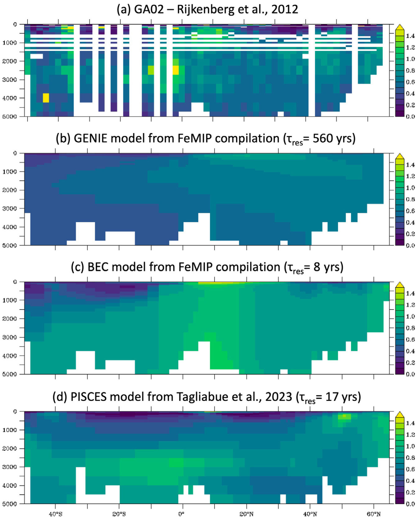
FIGURE 3. Comparison of model-predicted DFe distributions. (a) Observed DFe distribution along the GA02 section (Rijkenberg et al., 2012). (b,c) Predictions from two models included in the FeMIP intercomparison project (Tagliabue et al., 2016) include one with a long Fe residence time (τres) in which DFe exhibits clear water mass structure (b), and one with a short τres that captures sharp DFe source features. (d) A prediction from a newly configured state of the art model (Tagliabue et al., 2023a) accurately captures the observed distribution, with a relatively short τres. > High res figure

 

Probing Trace Element Inputs and Losses

Distributions of TEIs close to, and downstream of, boundary exchange regions (continental margins, the air-sea interface, mid-ocean ridges) provide clues about the magnitude of TEI fluxes across those boundaries that can be leveraged by models to construct budget estimates. Models that accurately reproduce observed TEI distributions are generally assumed to do so because they contain sources and sinks of realistic magnitude. A caveat is that, to some degree, unrealistic model sources and sinks can compensate one another—for instance, a source overestimate can be balanced by unrealistically rapid scavenging losses.

The first Fe model intercomparison project (FeMIP; Tagliabue et al., 2016) showed that 13 different models could all broadly reproduce the average concentrations observed from GEOTRACES data, while not reaching a consensus on the magnitude of external sources and scavenging losses. Models ranged from those with total sources on the order 1 Gmol yr^–1 and Fe residence times of hundreds of years to those with sources of >100 Gmol yr^–1 and residence times of 10 years or less. This has led to the impression that the observed DFe distribution does not place a strong constraint on the magnitude of Fe fluxes. However, a deeper comparison of model-​predicted DFe fields to observations (beyond just comparing mean concentrations) reveals significant differences between models with “slow” and “fast” Fe cycles. The former (small sources, slow scavenging) predict unrealistically smooth Fe fields with coherent water mass structures that are not observed in the GEOTRACES transects (Figure 3b), whereas the latter (large sources, fast scavenging) better resolve observed source features and the sharp Fe gradients around them (Figure 3c). Recent modeling studies that have most successfully reproduced observed DFe features tend to converge upon global Fe source estimates around 50–70 Gmol yr^–1 and residence times of 10–20 years (Figure 3d)—a much closer consensus than suggested by the FeMIP compilation (Pham and Ito, 2018; Tagliabue et al., 2023a). These models further agree that continental margin sediments are the dominant global Fe source to the ocean, while dust deposition and hydrothermal vents are secondary sources, albeit with significant regional imprints.

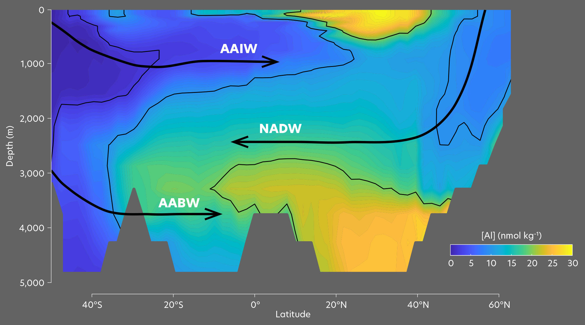
Complementary TEI tracers that share sources and sinks with Fe are increasingly being incorporated into prognostic models and studied with stand-alone transport matrix models to place additional constraints on Fe fluxes. For instance, Al has long been recognized as a powerful tracer of dust deposition from the atmosphere and has been the focus of both prognostic and inverse modeling studies (Van Hulten et al., 2014; Xu and Weber, 2021). The latter approach demonstrated that a source of 30–40 Gmol yr^–1 of soluble Al from dust was required to best match observed Al along a set of GEOTRACES sections, corresponding to a soluble Fe source of 5–10 Gmol yr^–1.

In addition to quantifying the magnitude of TEI sources and sinks, models have provided insights into the mechanisms and environmental controls on these processes. Often, the same conclusions have been reached independently from modeling of large-scale TEI distributions and from small-scale observational studies, building confidence that robust “general rules” have been discovered. For instance: (1) inverse modeling found that large-scale variability in dust solubility was required to match the global Al distribution with much higher solubility in remote regions with low atmospheric dust loading (Xu and Weber, 2021), consistent with acid-​leach experiments (Jickells et al., 2016); (2) two global Fe model studies demonstrated a better match to global GEOTRACES observations when benthic Fe sources were strongly amplified under low O₂ bottom-water conditions (Dale et al., 2015; Pham and Ito, 2018), consistent with flux chamber measurements on the Oregon shelf (Severmann et al., 2010); and (3) incorporation of Fe isotopes into a prognostic model demonstrated that distinct isotopic signatures must be resolved for Fe sourced from reductive and non-reductive sediments to match observed sections (König et al., 2021), consistent with pore-water measurements (Homoky et al., 2013).

Models have also been used to explore TEI removal processes, especially those associated with scavenging and the role of ligands. The earliest Fe models assumed a constant buffering of deep ocean DFe to 0.6 nM, presumed to represent a static oceanic ligand reservoir (Archer and Johnson, 2000); this was refined by later models to explicitly resolve the ligand complexation of Fe using equilibrium assumptions (Parekh et al., 2005). Present-day Earth system models still employ these parameterizations, and their assumptions about ligand concentrations can have important implications for atmospheric CO₂ (Tagliabue et al., 2014). Growing datasets for ligand concentrations and the recognition of greater variation in DFe concentrations led to the development of alternative approaches to modeling ligands, including empirical relationships that varied in response to DOC or O₂ (e.g., Pham and Ito, 2018) or even fully prognostic representations of ligand sources and sinks (Volker and Tagliabue, 2015). Comparing sophisticated Fe speciation models with time-series observations following dust deposition in the Mediterranean allowed the important roles of scavenging removal and competition with biological uptake to be revealed (Ye et al., 2011). Most recently, a comprehensive model-data synthesis exercise over the annual cycle at the Bermuda Atlantic Time-series Study site, spanning dissolved, ligand, and particulate Fe datasets, led to a revised model of the ocean iron cycle that placed less emphasis on stabilization of DFe by ligands and more on colloidal Fe aggregation with organic matter as a critical iron removal pathway (Tagliabue et al., 2023a).

 

Connecting Trace Metals to the Global Carbon Cycle

A key driver of research on micronutrients is their potential role in regulating the ocean carbon cycle via their impact on phytoplankton productivity. Insight into how micronutrients such as Fe can modulate the carbon cycle can be gleaned from observations, especially process studies (e.g. Boyd et al., 2007, 2012; Twining et al., 2021), but obtaining a large-scale holistic picture requires the use of prognostic global ocean biogeochemical models. Such tools can test hypothesized impacts of changes in micronutrient sources and internal cycling on carbon and macronutrients, oxygen, and primary production, as all components are interconnected in these models. A notable example here is the exploration of hydrothermal vent inputs of Fe and their impact on the global ocean carbon cycle.

At the launch of the GEOTRACES program, mid-ocean ridges were acknowledged as a potential external TEI source but were not considered to play a major role in driving the distribution of micronutrient trace metals and their impacts on the carbon cycle. However, new observations from the Southern Ocean emerging from the International Polar Year in 2008 indicated unexpected elevations in dissolved Fe in the vicinity of the Antarctic ridge crest (e.g., Klunder et al., 2011). Models were quickly adapted to explore the implications of this unforeseen Fe source, drawing on the link between hydrothermal Fe and mantle helium (Boyle and Jenkins, 2008; Fitzsimmons et al., 2014) to parameterize vent Fe inputs based on helium (He) input fields first developed for the Ocean Carbon Model Intercomparison Project (Dutay et al., 2004). Early work indicated that a significant enhancement in Fe was expected in the 2–3 km depth strata due to hydrothermal venting (Figure 4a) into the surface waters of the Southern Ocean (Figure 4b; Tagliabue et al., 2010). Furthermore, models with hydrothermal Fe were able to better reproduce GEOTRACES observations from the abyssal ocean. Follow-up studies in the South Atlantic demonstrated variation in the Fe:He ratios typical of slower spreading ridge systems (Saito et al., 2013), and the large-scale plume dispersing thousands of kilometers from the fast-​spreading East Pacific Rise captured by the GP16 voyage was not expected (Resing et al., 2015). Combined modeling and observational efforts that traced this plume across the Pacific explored the roles of external supply rates and internal processes that stabilize Fe against scavenging in explaining plume dispersal (Resing et al., 2015). This work, combined with inverse modeling exercises, estimated that hydrothermal Fe fuels up to 30% of Southern Ocean export production (Figure 4c; Resing et al., 2015; Tagliabue and Resing, 2016; Pasquier and Holzer, 2017). A set of more detailed model experiments focusing on the roles of different ridge systems led to the pinpointing of the ridges circling Antarctica as playing a key role in driving the impact on the carbon cycle (Figure 4a; Tagliabue and Resing, 2016).

 

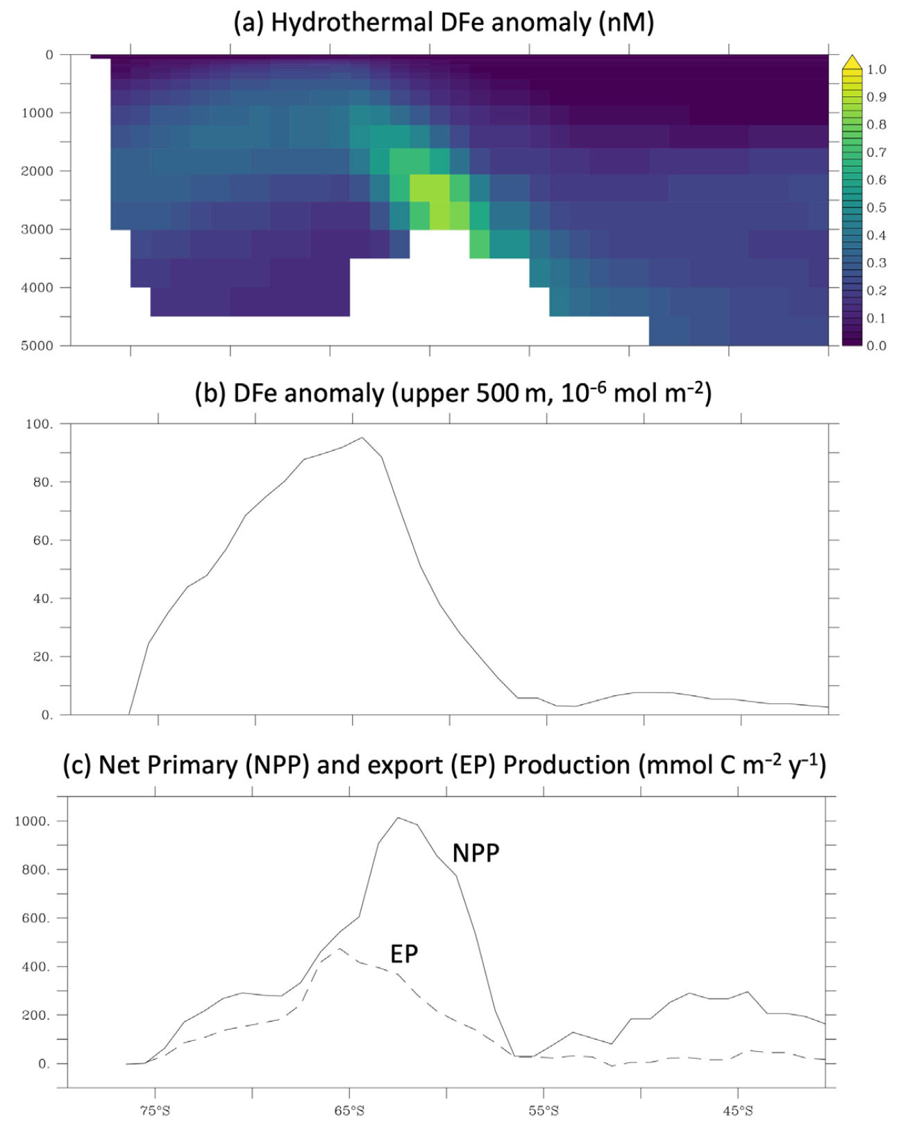
FIGURE 4. Impact of hydrothermal Fe on the ocean carbon cycle. (a) An example is shown here of the predicted distribution of hydrothermally sourced DFe in the Southern Ocean (nM, along 150°W), quantified as the difference between simulations with and without the vent source enabled, using the model of Tagliabue et al. (2023a). (b) An anomaly in integrated upper 500 m DFe due to hydrothermalism (10–6 mol Fe m–2) indicates the emergence of the hydrothermal DFe anomaly into the upper ocean at the Antarctic Divergence (upwelling center). (c) The net primary production (mmol m–2 yr–1, depth integrated, solid line) and carbon export (mmol m–2 yr–1, sinking flux across 100 m, dashed line) production plotted here is fueled specifically by hydrothermal Fe, again quantified as the difference between simulations with and without the vent source. > High res figure

 

Recent efforts to better quantify how the hydrothermal Fe supply regulates the ocean carbon cycle have focused on refining model parameterization of inputs and internal cycling processes. Due its role as a fingerprint for hydrothermally sourced waters, refining estimates of the mantle He source has been a particular focus area. The first helium input estimates linked the 400–1,000 mol He yr^–1 global source to ridge spreading rates (Dutay et al., 2004; Bianchi et al., 2010) and accordingly assumed greater hydrothermal supply along faster spreading ridges. More recently, an inverse modeling approach that leverages the Ocean Circulation Inverse Model physics and all available He measurements found that the total He supply likely lies at the low end of previous estimates, with inputs from Antarctic ridges reduced threefold (DeVries and Holzer, 2019). Assuming close coupling between the supplies of He and Fe implies that perhaps the role of Southern Ocean ridge systems, and hence the postulated impact of hydrothermal Fe on the carbon cycle, had been overestimated. Roshan et al. (2020) linked the new estimate of He inputs with a size-resolved model of hydrothermal Fe and optimized key parameters using the GP16 Pacific Ocean GEOTRACES transect. This model predicts that global hydrothermal Fe inputs largely originate on the East Pacific Rise and that there is very little hydrothermal Fe in the Southern Ocean, thanks to a combination of scavenging and weak Fe inputs from Antarctic ridges. Follow-up work with a full iron cycle model showed that, while low input rates along Antarctic ridges would indeed reduce the leverage of hydrothermal Fe on carbon export, they are not consistent with new observations of dissolved Fe from these systems (Tagliabue et al., 2022). These observations suggest that some Antarctic ridges could be a stronger source of Fe than would be expected from their He input, meaning that model source schemes for hydrothermal Fe may ultimately need to look beyond a simple link to He.

In addition to hydrothermal vents, modeling efforts have explored other aspects of how iron regulates the carbon cycle. For example, long-term Earth system model simulations run to the year 2300 under high emissions scenarios demonstrate a role for climate perturbation of the Fe budget in driving Southern Ocean nutrient depletion and low latitude declines in net primary production (Moore et al., 2018). Similarly, a range of model experiments show that climate-forced alterations to dust deposition have wide-reaching impacts on the biogeochemistry and carbon cycle of the Indian and Pacific Oceans (Pham and Ito, 2021; König et al., 2022). Models have long been used to assess the limited carbon sequestration potential and unintended biogeochemical consequences of purposeful ocean iron fertilization efforts (Oschlies et al., 2010; Tagliabue et al., 2023b). In this context, prognostic biogeochemical models will continue to be critical tools for quantifying the impacts of ocean iron fertilization proposals, especially regarding marine ecosystems. By coupling a global ocean biogeochemical model with an ecosystem model, recent work showed that ocean iron fertilization led to a very small increase in ocean carbon storage but amplified the negative impacts of climate change on ecosystems by a third (Tagliabue et al., 2023b). Recently, there has also been growing interest in the possible impact of other micronutrients beyond iron on the carbon cycle via potential regulation of phytoplankton growth rates and net primary production. To date, only Mn has been included as a directly limiting nutrient in ocean models, and its inclusion has been shown to lessen the response of the Southern Ocean biological carbon pump to the changes in Fe supply typical of the Last Glacial Maximum (Hawco et al., 2022). Coupled modeling of Fe and Mn limitations reveals how these micronutrients may interact via region-specific adjustments to phytoplankton physiology and affect the regional carbon cycle (Anugerahanti and Tagliabue, 2023). In the future, addressing the large-scale carbon cycle impacts of other potentially growth-limiting micronutrients, such as Zn, Co, and vitamin B12, will require use of more complex ocean models.

 

Outlook and Challenges

Modeling will remain an important tool in future trace element research, especially as the community’s focus increasingly shifts toward synthesis, process understanding, and linking TEIs to microbial ecology. Here, we discuss just two of many pressing future directions.

Toward TEI State Estimates: A “state estimate” represents our best understanding of the current state of a dynamic system given available observations and models. In marine biogeochemistry, a state estimate usually takes the form of a global, three-dimensional tracer distribution (e.g., a monthly climatology). As the observational phase of GEOTRACES enters its final stages, there is a growing need to synthesize the understanding of TEI distributions (and their uncertainties) that have emerged from the program as a set of state estimates. These would find broad applications in marine chemistry, but also beyond, including (1) guiding future observational efforts by identifying key regions of uncertainty; (2) adding trace element context to other datasets where TEIs cannot be measured directly, for example, comparison of biological rate measurements and genomic indicators to estimated micronutrient levels; (3) providing initialization fields and filling in “unresolved tracers” in ocean models, because not every model can explicitly resolve all micronutrient cycles, but accounting for their impacts on biological processes is desirable; and (4) providing information to policymakers, for instance, on the spread of anthropogenic trace element contaminants through the ocean. Given the sparseness of TEI measurements, GEOTRACES state estimates cannot simply be generated using the standard interpolation and objective mapping approach used for familiar data-rich state estimates like the World Ocean Atlas (hydrography, nutrients, oxygen) and the Global Ocean Data Analysis Project (carbon chemistry). Instead, they must ultimately rely on the three categories of models outlined in the section on Categories of TEI Models. Because machine learning models make the most direct use of observations, they are likely to be the most promising choice for state estimate generation. However, their ability to skillfully predict TEI distributions in regions with very few training data is not well understood, especially for short residence time elements that can have very patchy distributions. In these cases, mechanistic models that explicitly resolve the underlying processes may be considered more skillful gap-filling tools. A major intercomparison effort is needed to converge on the “best practices” for TEI state estimates.

Environmental Change: A key component of the GEOTRACES mission concerns the sensitivity of TEI cycles to environmental change (GEOTRACES Planning Group, 2006). While this can be documented and alluded to from field measurements, a global-scale assessment of how climate change may affect TEI cycling requires modeling efforts. The roles of changes in ocean circulation, environmental conditions, and external TEI inputs under different climate change scenarios can only be addressed using prognostic biogeochemical models that are forced by climate change scenarios. For longer residence time TEIs, such as Cd and Zn, we might expect more predictable changes that can be largely accounted for via the distribution of water masses. That said, in the upper ocean, where bio-​limiting roles will be felt, even long residence time elements such as these can display rapid changes in cycling, especially those mediated by phytoplankton uptake and zooplankton recycling, which may generate biogeochemical feedbacks (Richon and Tagliabue, 2019). TEIs with shorter residence times, such as Fe, will exhibit not only changes due to ocean circulation but also alterations due to their sources and elemental cycling throughout the ocean. These may include redistribution due to changes in mixing and nutrient limitation patterns at low latitudes (Misumi et al., 2014), as well as changes in Fe speciation due to temperature, pH, or oxygen perturbations that may affect removal processes, including the newly identified “colloidal shunt” (Tagliabue et al., 2023a). A critical area of focus will be the impacts of Fe on ocean biology, specifically potential adjustments in patterns of Fe limitation associated with climate variations (Browning et al., 2023). This will require refinement of the way in which phytoplankton Fe requirements, uptake, and limitation, as well as interactions with grazers and bacteria in the dynamic upper ocean, are included in models.

 

Acknowledgments

AT was supported by the European Research Council (Grant #724289), the Natural Environment Research Council (on grants NE/N009525/1, NE/S013547/1, and NE/X014908/1), and as part of the AtlantECO project, which has received funding from the European Union’s Horizon 2020 Framework Programme (HORIZON) under grant agreement no. 862923. TW was supported by the National Science Foundation through awards OCE-1658042 and OCE-2241744. The international GEOTRACES program is possible in part thanks to the support from the US National Science Foundation (Grant OCE-2140395) to the Scientific Committee on Oceanic Research (SCOR).

Tagliabue, A., and T. Weber. 2024. Novel insights into ocean trace element cycling from biogeochemical models. Oceanography 37(2):131–141, https://doi.org/​10.5670/oceanog.2024.418.

Anugerahanti, P., and A. Tagliabue. 2023. Process controlling iron-manganese regulation of the Southern Ocean biological carbon pump. Philosophical Transactions of the Royal Society A 381(2249), https://doi.org/10.1098/rsta.2022.0065.

Archer, D.E., and K. Johnson. 2000. A model of the iron cycle in the ocean. Global Biogeochemical Cycles 14(1):269–279, https://doi.org/​10.1029/​1999GB900053.

Arsouze, T., J.C. Dutay, F. Lacan, and C. Jeandel. 2009. Reconstructing the Nd oceanic cycle using a coupled dynamical-biogeochemical model. Biogeosciences 6(12):2,829–2,846, https://doi.org/​10.5194/​bg-6-2829-2009.

Bianchi, D., J.L. Sarmiento, A. Gnanadesikan, R.M. Key, P. Schlosser, and R. Newton. 2010. Low helium flux from the mantle inferred from simulations of oceanic helium isotope data. Earth and Planetary Science Letters 297:379–386, https://doi.org/​10.1016/​j.epsl.2010.06.037.

Boyd, P.W., T. Jickells, C.S. Law, S. Blain, E.A. Boyle, K.O. Buesseler, K.H. Coale, J.J. Cullen, H.J.W. de Baar, M. Follows, and others. 2007. Mesoscale iron enrichment experiments 1993–2005: Synthesis and future directions. Science 315(5812):612–617, https://doi.org/10.1126/science.1131669.

Boyd, P.W., R. Strzepek, S. Chiswell, H. Chang, J.M. DeBruyn, M. Ellwood, S. Keenan, A.L. King, E.W. Maas, S. Nodder, and others. 2012. Microbial control of diatom bloom dynamics in the open ocean. Geophysical Research Letters 39(18), https://doi.org/10.1029/2012GL053448.

Boyle, E.A., and W.K. Jenkins. 2008. Hydrothermal iron in the deep western South Pacific. Geochimica et Cosmochimica Acta 72:A107.

Broecker, W.S., T. Takahashi, and T. Takahashi. 1985. Sources and flow patterns of deep-ocean waters as deduced from potential temperature, salinity, and initial phosphate concentration. Journal of Geophysical Research: Oceans 90(C4):6,925–6,939, https://doi.org/​10.1029/JC090iC04p06925.

Browning, T.J., M.A. Saito, S.P. Garaba, X.C. Wang, E.P. Achterberg, C.M. Moore, A. Engel, M.R. Mcllvin, D. Moran, D. Voss, and others. 2023. Persistent equatorial Pacific iron limitation under ENSO forcing. Nature 621(7978):330–335, https://doi.org/​10.1038/​s41586-023-06439-0.

Bruland, K.W., G.A. Knauer, and J.H. Martin. 1978. Zinc in Northeast Pacific water. Nature 271(5647):741–743, https://doi.org/​10.1038/271741a0.

Dale, A.W., L. Nickelsen, F. Scholz, C. Hensen, A. Oschlies, and K. Wallmann. 2015. A revised global estimate of dissolved iron fluxes from marine sediments. Global Biogeochemical Cycles 29:691–707, https://doi.org/​10.1002/​2014GB005017.

de Baar, H.J., P.M. Saager, R.F. Nolting, and J. van der Meer. 1994. Cadmium versus phosphate in the world ocean. Marine Chemistry 46(3):261–281, https://doi.org/​10.1016/0304-4203(94)90082-5.

DeVries, T., and M. Holzer. 2019. Radiocarbon and helium isotope constraints on deep ocean ventilation and mantle-³He sources. Journal of Geophysical Research: Oceans 124(5):3,036–3,057, https://doi.org/10.1029/2018JC014716.

Dutay, J.C., P. Jean-Baptiste, J.M. Campin, A. Ishida, E. Maier-Reimer, R.J. Matear, A. Mouchet, I.J. Totterdell, Y. Yamanaka, K. Rodgers, and others. 2004. Evaluation of OCMIP-2 ocean models’ deep circulation with mantle helium-3. Journal of Marine Systems 48(1–4):15–36, https://doi.org/10.1016/​j.jmarsys.2003.05.010.

Eisenring, C., S.E. Oliver, S. Khatiwala, and G.F. de Souza. 2022. Influence of GEOTRACES data distribution and misfit function choice on objective parameter retrieval in a marine zinc cycle model. Biogeosciences 19(21):5,079–5,106, https://doi.org/​10.5194/bg-19-5079-2022.

Ellwood, M.J., and K.A. Hunter. 2000. The incorporation of zinc and iron into the frustule of the marine diatom Thalassiosira pseudonana. Limnology and Oceanography 45:1,517–1,524, https://doi.org/​10.4319/​lo.2000.45.7.1517.

Fitzsimmons, J.N., W.J. Jenkins, and E.A. Boyle. 2014. Distal transport of dissolved hydrothermal iron in the deep South Pacific Ocean. Proceedings of the National Academy of Sciences of the United States of America 111(47):16,654–16,661, https://doi.org/​10.1073/pnas.1418778111.

GEOTRACES Planning Group. 2006. GEOTRACES Science Plan. Scientific Committee on Oceanic Research, Baltimore, MD, https://geotracesold.sedoo.fr/libraries/documents/Science_plan.pdf.

Hawco, N.J., A. Tagliabue, and B.S. Twining. 2022. Manganese limitation of phytoplankton physiology and productivity in the Southern Ocean. Global Biogeochemical Cycles 36(11):e2022GB007382, https://doi.org/10.1029/2022GB007382.

Holzer, M., F.W. Primeau, T. DeVries, and R. Matear. 2014. The Southern Ocean silicon trap: Data-constrained estimates of regenerated silicic acid, trapping efficiencies, and global transport paths. Journal of Geophysical Research: Oceans 119(1):313–331, https://doi.org/​10.1002/​2013JC009356.

Homoky, W.B., S.G. John, T.M. Conway, and R.A. Mills. 2013. Distinct iron isotopic signatures and supply from marine sediment dissolution. Nature Communications 4:2143, https://doi.org/10.1038/ncomms3143.

Huang, Y.B., A. Tagliabue, and N. Cassar. 2022. Data-driven modeling of dissolved iron in the global ocean. Frontiers in Marine Science 9:837183, https://doi.org/10.3389/fmars.2022.837183.

Ito, T., and M.J. Follows. 2005. Preformed phosphate, soft tissue pump and atmospheric carbon dioxide. Journal of Marine Research 63:813–839.

Jickells, T.D., A.R. Baker, and R. Chance. 2016. Atmospheric transport of trace elements and nutrients to the oceans. Philosophical Transactions of the Royal Society A 374(2081):20150286, https://doi.org/10.1098/rsta.2015.0286.

John, S.G., H. Liang, T. Weber, T. DeVries, F. Primeau, K. Moore, M. Holzer, N. Mahowald, W. Gardner, A. Mishonov, and others. 2019. AWESOME OCIM: A simple, flexible, and powerful tool for modeling elemental cycling in the oceans. Chemical Geology 533:119403, https://doi.org/10.1016/​j.chemgeo.2019.119403.

John, S.G., R.L. Kelly, X.P. Bian, F.X. Fu, M.I. Smith, N.T. Lanning, H.D. Liang, B. Pasquier, E.A. Seelen, M. Holzer, and others. 2022. The biogeochemical balance of oceanic nickel cycling. Nature Geoscience 15(11):906–912, https://doi.org/10.1038/s41561-022-01045-7.

Khatiwala, S. 2007. A computational framework for simulation of biogeochemical tracers in the ocean. Global Biogeochemical Cycles 21(3), https://doi.org/​10.1029/​2007GB002923.

Klunder, M.B., P. Laan, R. Middag, H.J.W. De Baar, and J.C. van Ooijen. 2011. Dissolved iron in the Southern Ocean (Atlantic sector). Deep Sea Research Part II 58(25–26):2,678–2,694, https://doi.org/​10.1016/j.dsr2.2010.10.042.

König, D., T.M. Conway, M.J. Ellwood, W.B. Homoky, and A. Tagliabue. 2021. Constraints on the cycling of iron isotopes from a global ocean model. Global Biogeochemical Cycles 35(9):e2021GB006968, https://doi.org/10.1029/2021GB006968.

König, D., T.M. Conway, D.S. Hamilton, and A. Tagliabue. 2022. Surface ocean biogeochemistry regulates the impact of anthropogenic aerosol Fe deposition on the cycling of iron and iron isotopes in the North Pacific. Geophysical Research Letters 49(13):e2022GL098016, https://doi.org/​10.1029/​2022GL098016.

Liang, H.D., J.W. Moffett, and S.G. John. 2023. Toward a better understanding of the global ocean copper distribution and speciation through a data-constrained model. Global Biogeochemical Cycles 37(9):e2023GB007769, https://doi.org/​10.1029/2023GB007769.

Misumi, K., K. Lindsay, J.K. Moore, S.C. Doney, F.O. Bryan, D. Tsumune, and Y. Yoshida. 2014. The iron budget in ocean surface waters in the 20th and 21st centuries: Projections by the Community Earth System Model version 1. Biogeosciences 11(1):33–55, https://doi.org/​10.5194/bg-11-33-2014.

Moore, J.K., W.W. Fu, F. Primeau, G.L. Britten, K. Lindsay, M. Long, S.C. Doney, N. Mahowald, F. Hoffman, and J.T. Randerson. 2018. Sustained climate warming drives declining marine biological productivity. Science 359(6380):1,139–1,142, https://doi.org/10.1126/science.aao6379.

Oschlies, A., W. Koeve, W. Rickels, and K. Rehdanz. 2010. Side effects and accounting aspects of hypothetical large-scale Southern Ocean iron fertilization. Biogeosciences 7(12):4,017–4,035, https://doi.org/​10.5194/​bg-7-4017-2010.

Parekh, P., M.J. Follows, and E.A. Boyle. 2005. Decoupling of iron and phosphate in the global ocean. Global Biogeochemical Cycles 19(2), https://doi.org/​10.1029/2004GB002280.

Pasquier, B., and M. Holzer. 2017. Inverse-model estimates of the ocean’s coupled phosphorus, silicon, and iron cycles. Biogeosciences 14(18):4,125–4,159, https://doi.org/10.5194/bg-14-4125-2017.

Pasquier, B., and M. Holzer. 2018. The number of past and future regenerations of iron in the ocean and its intrinsic fertilization efficiency. Biogeosciences 15(23):7,177–7,203, https://doi.org/​10.5194/bg-15-7177-2018.

Pham, A.L.D., and T. Ito. 2018. Formation and maintenance of the GEOTRACES subsurface-dissolved iron maxima in an ocean biogeochemistry model. Global Biogeochemical Cycles 32(6):932–953, https://doi.org/10.1029/2017GB005852.

Pham, A.L.D., and T. Ito. 2021. Anthropogenic iron deposition alters the ecosystem and carbon balance of the Indian Ocean over a centennial timescale. Journal of Geophysical Research: Oceans 126(2):e2020JC016475, https://doi.org/​10.1029/2020JC016475.

Primeau, F. 2005. Characterizing transport between the surface mixed layer and the ocean interior with a forward and adjoint global ocean transport model. Journal of Physical Oceanography 35:545–564, https://doi.org/​10.1175/JPO2699.1.

Resing, J.A., P.N. Sedwick, C.R. German, W.J. Jenkins, J.W. Moffett, B.M. Sohst, and A. Tagliabue. 2015. Basin-scale transport of hydrothermal dissolved metals across the South Pacific Ocean. Nature 523:200–203, https://doi.org/10.1038/nature14577.

Richon, C., and A. Tagliabue. 2019. Insights into the major processes driving the global distribution of copper in the ocean from a global model. Global Biogeochemical Cycles 33(12):1,594–1,610, https://doi.org/10.1029/2019GB006280.

Rijkenberg, M.J.A., R. Middag, P. Laan, L.J.A. Gerringa, H.M. van Aken, V. Schoemann, J.T.M. de Jong, and H.J.W. de Baar. 2014. The distribution of dissolved iron in the West Atlantic Ocean. PLOS ONE 9(6):e101323, https://doi.org/10.1371/​journal.pone.0101323.

Roshan, S., and T. DeVries. 2017. Efficient dissolved organic carbon production and export in the oligotrophic ocean. Nature Communications 8:2036, https://doi.org/10.1038/s41467-017-02227-3.

Roshan, S., T. DeVries, J.F. Wu, and G.D. Chen. 2018. The internal cycling of zinc in the ocean. Global Biogeochemical Cycles 32(12):1,833–1,849, https://doi.org/10.1029/2018GB006045.

Roshan, S., T. DeVries, J. Wu, S. John, and T. Weber. 2020. Reversible scavenging traps hydrothermal iron in the deep ocean. Earth and Planetary Science Letters 542:116297, https://doi.org/10.1016/​j.epsl.2020.116297.

Roshan, S., and T. DeVries. 2021. Global contrasts between oceanic cycling of cadmium and phosphate. Global Biogeochemical Cycles 35(6):e2021GB006952, https://doi.org/​10.1029/2021GB006952.

Saito, M.A., A.E. Noble, A. Tagliabue, T.J. Goepfert, C.H. Lamborg, and W.J. Jenkins. 2013. Slow-spreading submarine ridges in the South Atlantic as a significant oceanic iron source. Nature Geoscience 6:775–779, https://doi.org/10.1038/ngeo1893.

Seferian, R., S. Berthet, A. Yool, J. Palmieri, L. Bopp, A. Tagliabue, L. Kwiatkowski, O. Aumont, J. Christian, J. Dunne, and others. 2020. Tracking improvement in simulated marine biogeochemistry between CMIP5 and CMIP6. Current Climate Change Reports 6(3):95–119, https://doi.org/​10.1007/s40641-020-00160-0.

Severmann, S., J. McManus, W.M. Berelson, and D.E. Hammond. 2010. The continental shelf benthic iron flux and its isotope composition. Geochimica et Cosmochimica Acta 74:3,984–4,004, https://doi.org/​10.1016/j.gca.2010.04.022.

Sieber, M., N.T. Lanning, X. Bian, S.C. Yang, S. Takano, Y. Sohrin, T.S. Weber, J.N. Fitzsimmons, S.G. John, and T.M. Conway. 2023. The importance of reversible scavenging for the marine Zn cycle evidenced by the distribution of zinc and its isotopes in the Pacific Ocean. Journal of Geophysical Research: Oceans 128(4):e2022JC019419, https://doi.org/​10.1029/2022JC019419.

Tagliabue, A., L. Bopp, J.C. Dutay, A.R. Bowie, F. Chever, P. Jean-Baptiste, E. Bucciarelli, D. Lannuzel, T. Remenyi, G. Sarthou, and others. 2010. Hydrothermal contribution to the oceanic dissolved iron inventory. Nature Geoscience 3(4):252–256, https://doi.org/​10.1038/ngeo818.

Tagliabue, A., R.G. Williams, N. Rogan, E.P. Achterberg, and P.W. Boyd. 2014. A ventilation-​based framework for dissolved iron in the ocean. Geophysical Research Letters 41(20):7,227–7,236, https://doi.org/10.1002/2014GL061066.

Tagliabue, A., and J. Resing. 2016. Impact of hydrothermalism on the ocean iron cycle. Philosophical Transactions of the Royal Society A 374(2081):20150291, https://doi.org/10.1098/rsta.2015.0291.

Tagliabue, A., O. Aumont, R. Death, J.P. Dunne, S. Dutkiewicz, E. Galbraith, K. Misumi, J.K. Moore, A. Ridgwell, E. Sherman, and others. 2016. How well do global ocean biogeochemistry models simulate dissolved iron distributions? Global Biogeochemical Cycles 30(2):149–174, https://doi.org/​10.1002/​2015GB005289.

Tagliabue, A., A.R. Bowie, P.W. Boyd, K.N. Buck, K.S. Johnson, and M.A. Saito. 2017. The integral role of iron in ocean biogeochemistry. Nature 543(7643):51–59, https://doi.org/​10.1038/nature21058.

Tagliabue, A., N.J. Hawco, R.M. Bundy, W.M. Landing, A. Milne, P.L. Morton, and M.A. Saito. 2018. The role of external inputs and internal cycling in shaping the global ocean cobalt distribution: Insights from the first cobalt biogeochemical model. Global Biogeochemical Cycles 32(4):594–616, https://doi.org/​10.1002/2017GB005830.

Tagliabue, A., A.R. Bowie, T. DeVries, M.J. Ellwood, W.M. Landing, A. Milne, D.C. Ohnemus, B.S. Twining, and P.W. Boyd. 2019. The interplay between regeneration and scavenging fluxes drives ocean iron cycling. Nature Communications 10:4960, https://doi.org/10.1038/s41467-019-12775-5.

Tagliabue, A., A.R. Bowie, T. Holmes, P. Latour, P. Van Der Merwe, M. Gault-Ringold, K. Wuttig, and J.A. Resing. 2022. Constraining the contribution of hydrothermal iron to Southern Ocean export production using deep ocean iron observations. Frontiers in Marine Science 9:754517, https://doi.org/​10.3389/​fmars.2022.754517.

Tagliabue, A., K.N. Buck, L.E. Sofen, B.S. Twining, O. Aumont, P.W. Boyd, S. Caprara, W.B. Homoky, R. Johnson, D. König, and others. 2023a. Authigenic mineral phases as a driver of the upper-ocean iron cycle. Nature 620(7972):104–109, https://doi.org/10.1038/s41586-023-06210-5.

Tagliabue, A., B.S. Twining, N. Barrier, O. Maury, M. Berger, and L. Bopp. 2023b. Ocean iron fertilization may amplify climate change pressures on marine animal biomass for limited climate benefit. Global Change Biology 29(18):5,250–5,260, https://doi.org/10.1111/gcb.16854.

Twining, B.S., and S.B. Baines. 2013. The trace metal composition of marine phytoplankton. Annual Review of Marine Science 5:191–215, https://doi.org/​10.1146/annurev-marine-121211-172322.

Twining, B.S., O. Antipova, P.D. Chappell, N.R. Cohen, J.E. Jacquot, E.L. Mann, A. Marchetti, D.C. Ohnemus, S. Rauschenberg, and A. Tagliabue. 2021. Taxonomic and nutrient controls on phytoplankton iron quotas in the ocean. Limnology and Oceanography Letters 6(2):96–106, https://doi.org/​10.1002/lol2.10179.

van Hulten, M.M.P., A. Sterl, A. Tagliabue, J.C. Dutay, M. Gehlen, H.J.W. de Baar, and R. Middag. 2013. Aluminium in an ocean general circulation model compared with the West Atlantic Geotraces cruises. Journal of Marine Systems 126:3–23, https://doi.org/​10.1016/j.jmarsys.2012.05.005.

van Hulten, M.M.P., A. Sterl, R. Middag, H.J.W. De Baar, M. Gehlen, J.C. Dutay, and A. Tagliabue. 2014. On the effects of circulation, sediment resuspension and biological incorporation by diatoms in an ocean model of aluminium. Biogeosciences 11:3,757–3,779, https://doi.org/​10.5194/bg-11-3757-2014.

van Hulten, M., J.C. Dutay, and M. Roy-Barman. 2018. A global scavenging and circulation ocean model of thorium-230 and protactinium-231 with improved particle dynamics (NEMO-ProThorP 0.1). Geoscientific Model Development 11(9):3,537–3,556, https://doi.org/​10.5194/​gmd-11-3537-2018.

Vance, D., S.H. Little, G.F.D. Souza, S. Khatiwala, M.C. Lohan, and R. Middag. 2017. Silicon and zinc biogeochemical cycles coupled through the Southern Ocean. Nature Geoscience 10:202–206, https://doi.org/10.1038/ngeo2890.

Volker, C., and A. Tagliabue. 2015. Modeling organic iron-binding ligands in a three-​dimensional biogeochemical ocean model. Marine Chemistry 173:67–77, https://doi.org/10.1016/​j.marchem.​2014.11.008.

Weber, T., S. John, A. Tagliabue, and T. DeVries. 2018. Biological uptake and reversible scavenging of zinc in the global ocean. Science 361(6397):72–76, https://doi.org/10.1126/science.aap8532.

Weber, T., N.A. Wiseman, and A. Kock. 2019. Global ocean methane emissions dominated by shallow coastal waters. Nature Communications 10(1):4584, https://doi.org/10.1038/s41467-019-12541-7.

Xu, H., and T. Weber. 2021. Ocean dust deposition rates constrained in a data-assimilation model of the marine aluminum cycle. Global Biogeochemical Cycles 35(9):e2021GB007049, https://doi.org/​10.1029/​2021GB007049.

Yang, S., B.X. Chang, M.J. Warner, T.S. Weber, A.M. Bourbonnais, A.E. Santoro, A. Kock, R.E. Sonnerup, J.L. Bullister, S.T. Wilson, and others. 2020. Global reconstruction reduces the uncertainty of oceanic nitrous oxide emissions and reveals a vigorous seasonal cycle. Proceedings of the National Academy of Sciences of the United States of America 117(22):11,954–11,960, https://doi.org/​10.1073/​pnas.1921914117.

Ye, Y., T. Wagener, C. Völker, C. Guieu, and D.A. Wolf-Gladrow. 2011. Dust deposition: Iron source or sink? A case study. Biogeosciences 8(8):2,107–2,124, https://doi.org/10.5194/bg-8-2107-2011.

This is an open access article made available under the terms of the Creative Commons Attribution 4.0 International License (https://creativecommons.org/licenses/by/4.0/), which permits use, sharing, adaptation, distribution, and reproduction in any medium or format as long as users cite the materials appropriately, provide a link to the Creative Commons license, and indicate the changes that were made to the original content. Images, animations, videos, or other third-party material used in articles are included in the Creative Commons license unless indicated otherwise in a credit line to the material. If the material is not included in the article’s Creative Commons license, users will need to obtain permission directly from the license holder to reproduce the material.