An 18-month deployment of moored sensors in Iceland Basin allows characterization of near-inertial (frequencies near the Coriolis frequency f with periods of ~14 h) internal gravity wave generation and propagation in a region with an active mesoscale eddy field and strong seasonal wind and heat forcing. The seasonal cycle in surface forcing deepens the mixed layer in winter and controls excitation of near-​inertial energy. The mesoscale eddy field modulates near-inertial wave temporal, horizontal, and vertical scales, as well as propagation out of the surface layer into the deep permanent pycnocline. Wind-forced near-inertial energy has the most active downward propagation within anticyclonic eddies. As oceanic surface and bottom boundaries act to naturally confine the propagation of internal waves, the vertical distribution of these waves can be decomposed into a set of “standing” vertical modes that each propagate horizontally at different speeds. The lowest modes, which propagate quickly away from their generation sites, are most enhanced when the mixed layer is deep and are generally directed southward.

Photo credit: Manish Devana. > High res figure

Introduction

Wind forcing at the ocean surface is the main mechanism for generating near-​inertial waves (NIWs), which have an intrinsic frequency near the resonant Coriolis frequency f = 2ψsin(ϕ), where ψ is Earth’s rotation rate and ϕ is latitude. Much like surface ripples radiating away from a pebble dropped into water, wind-generated near-inertial waves radiate away from their generation region through a range of vertical and horizontal scales. However, unlike surface ripples, internal waves can propagate both horizontally and vertically, with the surface and bottom boundaries of the ocean limiting their propagation. A propagating wave can be decomposed into vertical modes that vary from fast-​moving equatorward-​propagating low modes, which are typically large-scale waves with horizontal wavelengths O(100) km and vertically standing patterns of oscillating horizontal currents (D’Asaro, 1985; Garrett, 2001; Alford, 2003b; Simmons and Alford, 2012), to slow-moving waves of intermediate to small vertical and horizontal scales that dominate internal wave energy and shear in the deep ocean (Müller et al., 1978; Pinkel, 1985; Kunze et al., 1990; Alford et al., 2017; Waterhouse et al., 2022). The lowest-​mode NIWs (generally modes 1 and 2) contain as much as half of the near-​​inertial energy and energy flux (D’Asaro et al., 1995; Alford, 2003a; Simmons and Alford, 2012; Raja et al., 2022) and distribute this energy far from their sources (Gill, 1984; Silverthorne and Toole, 2009; Alford, 2003a; Simmons and Alford, 2012). Intermediate-scale near-​inertial waves, which can also be generated through wave-wave (McComas and Bretherton, 1977; McComas and Müller, 2000; Henyey et al., 1986; Le Boyer and Alford, 2021) or wave-mean flow interactions (Kunze, 1985; Bühler and McIntyre, 2005; Rainville and Pinkel, 2006), contain shear that mediates the transfer of energy from large to dissipative scales (e.g., Gregg, 1989). The increased vertical shear associated with NIWs causes direct impacts on global ocean energy budgets (Kunze, 2017a) through enhanced turbulent mixing that affects various aspects of the ocean-​atmosphere climate system from the meridional overturning circulation (Kunze, 2017b) to the oceanic carbon cycle (Song et al., 2019) to long-term climate variability (Jochum et al., 2013).

Given the large scales over which low-mode NIWs propagate, the fate of these waves can be altered through interactions at generation, and during propagation, by energetic mesoscale activity. Oceanic mesoscale and associated eddies are often referred to as ocean “weather,” typically defined as having eddy scales less than 100 km and timescales of months. Downward propagation of NIWs into the thermocline is modulated by mesoscale vorticity (Kunze, 1985; Young and Jelloul, 1997), as evidenced in the relatively inconsistent seasonality of NIW downward energy fluxes (Park and Watts, 2005). Mesoscale eddies affect NIW behavior through their vorticity ζ modifying the effective inertial frequency f_e = f + ζ/2 (Kunze 1985; Elipot et al., 2010; Alford et al., 2013). Eddies have been found to focus near-inertial waves into anticyclones (Kunze, 1985), accelerate their downward propagation (e.g., Lee and Niiler, 1998; Halle and Pinkel, 2003; Rainville and Pinkel, 2004; Yu et al., 2022; Essink et al., 2022), and trap them at the edge of fronts (Kunze and Sanford, 1984; Weller, 1985; Zhong and Bracco, 2013). Additionally, eddies can control where NIWs dissipate (Kunze et al., 1995; Whalen et al., 2018). The observations presented in this paper aim to understand how mesoscale vorticity modulates the energy pathway of near-inertial inputs by investigating the vertical structure and energy flux of seasonally variable NIWs.

The Office of Naval Research (ONR) Near-Inertial Shear and Kinetic Energy in the North Atlantic experiment (NISKINe) was designed to study the full life cycle of near-inertial waves from generation through propagation to dissipation in a region with storm tracks and an energetic eddy kinetic energy (EKE) field. EKE in Iceland Basin is stronger in summer than in winter (Rieck et al., 2015), while wind forcing is stronger in winter than in summer. Other detailed studies on NISKINe field and modeling components can be found in Asselin and Young (2020), Thomas et al. (2020, 2023, and 2024, in this issue), Klenz et al. (2022), Kunze et al. (2023), and Girton et al. (2024, in this issue).

 

Moored Observations

One component of NISKINe included deployment of three full-depth moorings in a region of enhanced EKE in Iceland Basin (Figure 1). The moorings were deployed for 18 months, from May 5, 2019, until October 5, 2020, in a triangular array separated by 15 km and centered around 59°6'N, 21°12'W in approximately 2,800-meters water depth. Moorings were arranged in a triangle to allow for future estimates of energy exchange between near-inertial waves and the mesoscale circulation. The location of the NISKINe array was chosen based on the area’s consistent EKE signal (Figure 1). The spacing between moorings was chosen to resolve mesoscale eddy shears.

 

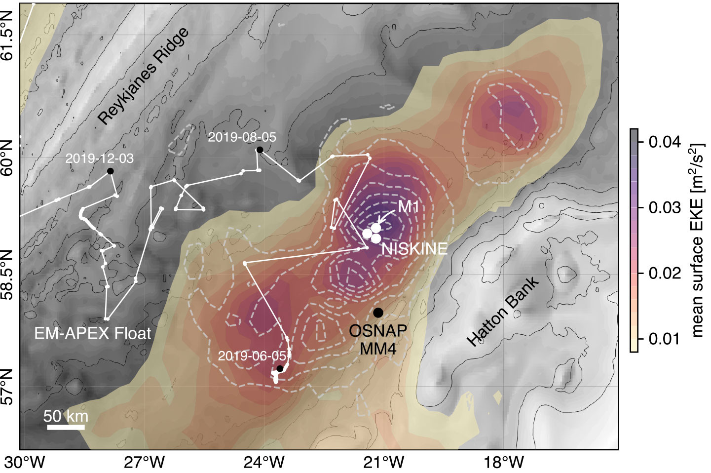
FIGURE 1. Locations of three NISKINe moorings deployed from May 2019 to October 2020 are indicated by white circles, with the northmost mooring labeled M1. OSNAP mooring MM4 (black circle) was deployed from July 2014 to June 2016. The white line shows the trajectory of an EM-APEX float deployed near 57°N, 24°W on June 5, 2019 (marked together with two later timestamps), and small white dots give individual float locations spaced by varying periods (Irminger Sea portion not shown). Color shading shows surface eddy kinetic energy (EKE) in the Iceland Basin based on satellite sea level anomaly data between 2005 and 2020. Light gray dashed contours show the covariance pattern between EKE and the dominant mode of EKE variability (based on empirical orthogonal function analysis) in the area. > High res figure

 

The primary mooring, M1, was equipped with acoustic Doppler current Profilers (ADCPs) sampling velocity continuously over the upper 1,500 m of the water column. An additional point measurement of velocity 26 m above the seafloor stopped working about two weeks after deployment due to instrument failure. Temperature and salinity were measured concurrently with Sea-Bird SBE 37 CTDs at 47, 170, 316, 594, and 2,850 m nominal depths. Temperature was recorded with SBE 56 and RBR Solo thermistors spaced 5 to 10 m in the upper 200 m and more coarsely distributed with spacing varying from 20 to 150 m down to 1,500 m depth (Figure 2a). In addition, turbulence-measuring χ-pods (Moum and Nash, 2009; Lien and Sanford, 2019) were attached from 100 m to 820 m depth. Only velocity and hydrography observations from M1 will be detailed here with quantification of lateral structure, evolution of energetics across the mooring array, and turbulence observations to be detailed in forthcoming papers.

At times, the moorings were exposed to high current velocities in the strongly eddying North Atlantic Current, so they experienced periods of sustained knockdown of up to 400 m due to high drag. These knockdown events are noted in Figure 2a–c as missing near-​surface current and temperature measurements. Pressure sensors on the moorings allow remapping the time series to constant depths. Vertical mooring excursions occurred at frequencies low enough that they did not appreciably affect depth-​gridded data products.

 

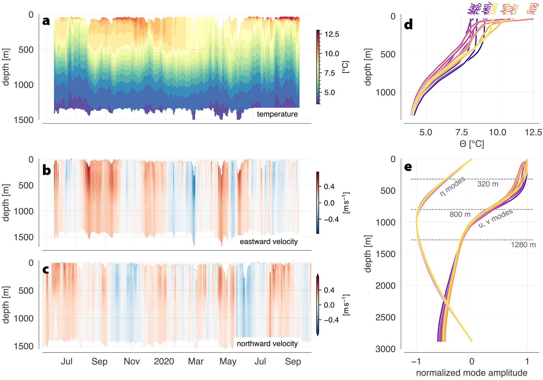
FIGURE 2. Seasonal cycles of temperature (a,d), horizontal velocity (u,v) (b,c) and mode-1 vertical profiles for displacement η and horizontal velocity (e) at NISKINe mooring M1. > High res figure

 

In addition to the NISKINe mooring array, a full-depth mooring from the Overturning in the Subpolar North Atlantic Program (OSNAP; mooring MM4; Figure 1) was included in the analysis to estimate low-mode near-​inertial internal-wave energy flux 100 km south of the NISKINe array between July 2014 and June 2016. While the OSNAP array was deployed to address meridional overturning fluxes in the subpolar North Atlantic (Lozier et al., 2019), a subset of its data also resolves low-mode near-​inertial wave fluxes (e.g., Vic et al., 2021). Although this mooring did not overlap in time with the NISKINe array, it provides information on seasonal variability in the Iceland Basin south of the NISKINe study area.

 

Seasonal Cycles of Background Fields

To quantify the effect of seasonal winds at the NISKINe mooring array, mixed-layer depth, near-inertial wind-work, and mesoscale satellite altimetry EKE and vorticity are calculated as described below. The oceanic mixed layer is a weakly stratified region in the upper ocean where there is little variation in temperature, salinity, or density with depth (Kara et al., 2000). Near-inertial wind-work is defined as transfer of kinetic energy from atmosphere to ocean at near-inertial frequency (e.g., Simmons and Alford, 2012; Torres et al., 2022). Vorticity estimates the rate of fluid rotation and is often quantified in the ocean as “normalized vorticity,” which describes the rate of fluid rotation normalized by Earth’s rotation (in this case by the Coriolis frequency f).

 

Mixed-Layer Depth

Mixed-layer depth (MLD) is typically calculated based on vertical profiles of density, temperature, or salinity (Thomson and Fine, 2003). From observations at mooring M1 (Figure 2a), an MLD time series is based on a temperature threshold of 0.2°C. In general, the threshold method identifies the depth at which the temperature profile changes by a predefined amount (the threshold value, 0.2°C) relative to a near-surface reference value. A density-based threshold could not be applied because most measurements on the mooring were temperature only. Time series from the few moored CTDs (not shown) indicate considerable isopycnal variability in temperature and salinity, complicating direct mapping of temperature to density.

The temperature-threshold-based MLD time series, calculated using the upper­most moored temperature record as the near-surface reference value, shows considerable deviation during mooring knockdown periods from Argo MLD climatology (Holte et al., 2017) interpolated to the mooring array (Figure 3c). Calculating MLD with mooring data alone proved to be elusive due to intermittent mooring knockdown and missing hydrography measurements in the upper 40 m. Comparison with satellite sea surface temperature (SST; Figure 3a) shows large differences between warmest temperatures observed by the M1 mooring and temperature at the ocean surface during summer months and during mooring knockdown. Therefore, when mooring knockdown exceeded 50 m or satellite SST deviated by more than 1.5°C from the uppermost moored temperature record, mooring MLD was replaced with Argo MLD climatology. Figure 3d shows the final MLD product derived for this NISKINe deployment.

 

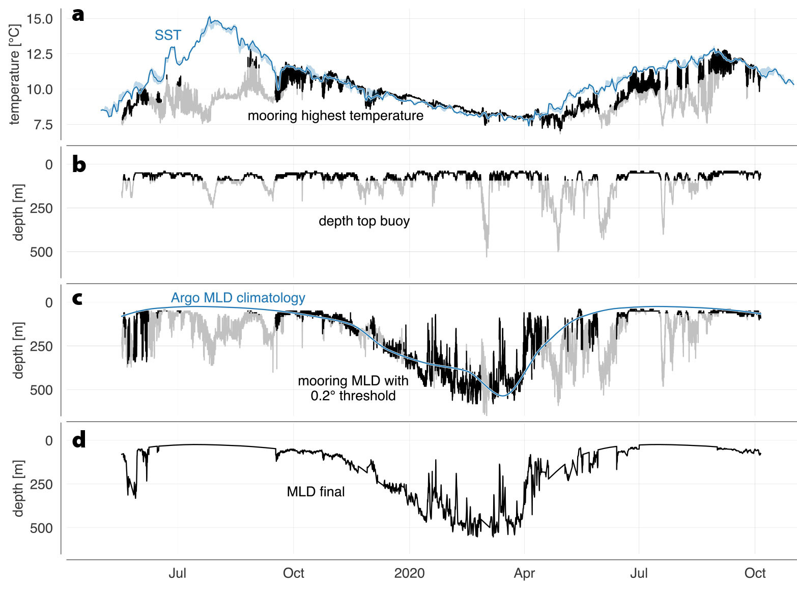
FIGURE 3. Mixed-layer depth calculation components and resulting time-​series. (a) Satellite sea surface temperature (SST, blue line), including average maximum and minimum temperature over a 20 km radius around mooring M1 (blue shading) and warmest temperature observed by the mooring (black line). Periods when SST differed by more than 1.5°C from the mooring observations are shown in gray. (b) Depth of the top-most mooring element, indicating mooring knockdown. Periods when the top buoy was deeper than 100 m are shown in gray. (c) Mixed-layer depth calculated from all temperature observations on the mooring based on a 0.2°C threshold. Periods where either SST differed by more than 1.5°C or the top float was deeper than 100 m are shown in gray. Argo mixed-layer depth climatology (Holte et al., 2017) for the mooring is shown in blue. (d) Combined product of moored temperature-based mixed-layer depth and Argo mixed-layer depth climatology (see text for details). > High res figure

 

MLD follows a seasonal cycle of deepening starting in early to mid fall, with a persistent winter remnant layer between 500 and 600 m (peaking in March), and a rapid return to less than 50 m at the beginning of summer (Figure 3d). MLD broadly agrees with climatology. However, a 400 m thick mixed layer persisted longer than was seen in climatology in both 2019 and 2020 (Figure 3c). The summer mixed layer forms a shallow seasonal pycnocline that overlies remnants of the deep winter mixed layer (Figure 2d). The deep winter mixed layer slowly restratifies starting at the cessation of deep winter convection in April and lasts until deep convection onset in December (Figure 2d; see also Box 1 and Figure 7 with buoyancy frequency N from EM-APEX float observations showing similar behavior). As pointed out by Kunze et al. (2023), restratification below the seasonal pycnocline may be explained by vertical mixing.

 

Near-Inertial Wind-Work

Surface wind stress and near-inertial wind-work have clear seasonal cycles, each with a minimum in summer and a maximum in winter (Figure 4a–c). We use wind data from the European Centre for Medium-Range Weather Forecasting (ECMWF) ERA5 reanalysis interpolated to the M1 mooring location. Wind stress τ is calculated as

with air density ρ_a, drag coefficient C_D, and relative wind speed u_r = u₁₀ – u_s. Here, u₁₀ is the ERA5 wind speed (10 m above sea level), and u_s is the ocean surface velocity taken from the moored velocity record in the mixed layer. Following Vic et al. (2021), we apply a correction factor to the calculation of u_r to account for current feedback on wind stress not taken into account in reanalysis products (Kelly and Thompson, 2002; Renault et al., 2020): u_r = u₁₀ – (1 – s_w)u_s where s_w = 0.3 is the globally averaged value of the current-​wind coupling coefficient.

Near-inertial wind-work Π_NI is calculated as

where  denotes inertial mixed-layer currents and  near-inertial wind stress that are obtained by band-pass filtering around the inertial frequency (f = 1.248 × 10^–4 [s^–1], with a bandwidth factor c = 1.06). The bandwidth factor c is chosen to satisfy cf < c^–1 ω_SD so as to separate semidiurnal tidal and inertial bands. Due to the proximity of inertial and semidiurnal frequencies (ω_SD = 1.13f) in the Iceland Basin, the pass band used for filtering is narrower than the customary c = 1.25 factor (e.g., Alford, 2003b).

 

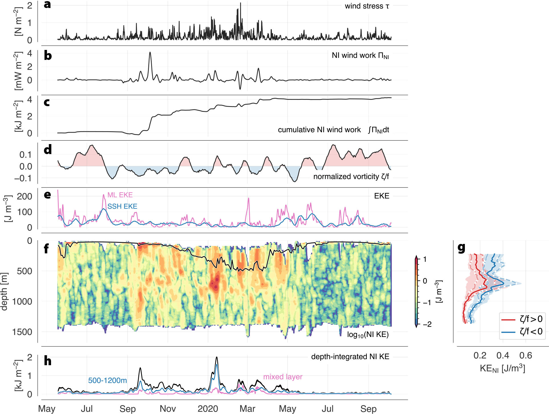
FIGURE 4. Surface forcing, upper ocean vorticity, upper ocean eddy kinetic energy, and near-inertial kinetic energy at mooring M1. (a) Surface wind stress τ from ERA-5 reanalysis. (b) Near-inertial wind-work ΠNI. (c) Cumulative near-inertial wind-work over the mooring deployment period. (d) Surface normalized vorticity ζ/f. (e) Estimates of surface eddy kinetic energy based on mixed-layer-averaged velocity (pink) and satellite-altimetry-derived sea surface height anomaly (blue). (f) Near-inertial kinetic energy. The black line shows mixed-layer depth from Figure 3d. (g) Vertical profiles of time-mean near-​inertial kinetic energy segregated into positive (red) and negative (blue) normalized vorticity ζ/f. Shading indicates 95% confidence intervals around the mean profiles based on a seven-day decorrelation timescale yielding 72 degrees of freedom in the 506-day-long time series. Only depths with less than 10% gaps due to mooring knockdown were included in the mean. Solid lines show overall means. Dashed profiles were calculated from near-inertial kinetic energy during the top 50 percentile of wind stress at the mooring site. Dash-dotted profiles were calculated from data during the lower 50 percentile of wind stress. (h) Near-inertial kinetic energy depth-integrated over the full water column (black), the mixed layer (pink), and between 500 m and 1,200 m depth (blue). > High res figure

 

Average near-inertial wind-work from May 2019 to October 2020 was 0.12 mW m^–2. During individual winter storm events, near-​inertial wind-work exceeded 2 mW m^–2. Cumulative near-inertial wind-work over the NISKINe deployment period was 4 kJ m^–2 (Figure 4c). Total global near-inertial wind-work of about 0.3 TW (Alford, 2020) translates to a global average of about 0.8 mW m^–2 or 25 kJ m^–2 annual wind-work. Thus, near-inertial wind-work at the NISKINe site is a factor of six smaller than the global average.

 

Eddy Kinetic Energy

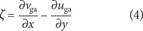
Mesoscale EKE in the Iceland Basin is concentrated over the deeper part of the basin (Figure 4e). It is calculated from satellite-altimetry-derived geostrophic velocities u_ga as

with lateral resolution of 0.25° or 28 km. For comparison, mixed-layer eddy kinetic energy (EKE_ML) is calculated from three-day low-pass-filtered velocity observations at mooring M1 (Figure 4e). EKE_ML generally follows the pattern of EKE but has higher amplitudes. Satellite-altimetry-derived geostrophic velocities are known to underestimate true geostrophic velocities because of finite resolution (Chelton et al., 2019), but the general match of high and low EKE from the two estimates gives us confidence in the satellite-​altimetry inference for this region. The seasonal cycle in surface EKE peaks in May (Figure 4e). Seasonal EKE variance is mostly focused on the center of Iceland Basin (dashed gray contours in Figure 1). EKE seasonality is a general feature of both the Atlantic and Pacific that may be related to upscale energy transfer from submesoscale variability (Sasaki et al., 2017; Naveira Garabato et al., 2022), seasonal variations in surface heat-fluxes, and associated thermocline changes (Rieck et al. 2015), or to a seasonal cycle in wind forcing and momentum removal at the mesoscale (Rai et al., 2021).

 

Vorticity

Relative vorticity is calculated from satellite-​altimetry-derived geostrophic velocity anomalies as

and normalized by the local inertial frequency f as ζ/f, which is referred to as normalized vorticity in the following. Direct estimates of vorticity from the triangular mooring array require careful processing (e.g., Lien and Müller, 1992) and will be included in future work.

Vorticity amplitudes at the mooring sites follow the seasonal cycle of surface EKE with enhanced vorticity in summer (Figure 4d). A 2005–2020 normalized vorticity average displays standing eddies in Iceland Basin with an anti­cyclonic eddy with ≈ –0.025 south of the mooring array and a cyclonic eddy to the north with ≈ +0.02 (not shown). The persistent anticyclonic eddy, referred to as “PRIME eddy” in previous studies (Martin et al., 1998; Wade and Heywood, 2001), is characterized by a cold core. The northmost mooring M1 was located in positive long-term mean vorticity, the southmost mooring M2 in negative mean vorticity, and M3 in the transition. From May 2019 to October 2020, average vorticity was positive at all moorings, with a meridional vorticity gradient of the same sign and about twice as large as the long-term average. The average meridional gradient in vorticity for this time was an order of magnitude larger than the planetary meridional inertial frequency gradient β.

 

Seasonal Variability

Seasonal Variation of Velocity and Kinetic Energy

Over the duration of the NISKINe deployment, surface velocities were generally deep-reaching, with currents exceeding 0.4 m s^–1 for sustained periods (Figure 2b,c). Near-inertial kinetic energy

is enhanced in winter (Figure 4f). Depth extent of the initial response to enhanced NI wind-work increases as the mixed layer deepens from January through March, and near-inertial kinetic energy content in the water column is generally larger when the mixed layer is deeper (Figure 4h, black). Near-inertial kinetic energy below the permanent pycnocline at around 500 m depth is largely independent of mixed-layer depth (Figure 4h, blue). Winter-enhanced near-inertial KE events observed from the mooring differ from summer-enhanced KE events observed by EM-APEX floats (see Box 1, Figure 7), likely due to the different modal content captured by each platform, with low modes dominating the near-full-water-column moored observations and higher modes (>8) dominating the EM-APEX float measurements (which sample to 800 m depth, above the first zero crossing of the first ~7 modes).

Near-inertial kinetic energy associated with negative normalized vorticity (anticyclones) is twice that in positive normalized vorticity (cyclones; Figure 4g), likely due to vorticity refraction, which focuses and traps near-inertial energy in anticyclonic vorticity (Elipot et al., 2010), then amplifies it at critical layers at the bases of anticyclones (Kunze et al.,1995; Lelong et al., 2020; Yu et al., 2022).

Two high near-inertial kinetic energy events below the permanent pycnocline during September 2019 and January 2020 stand out. Both coincide with negative vorticity and were observed across the triangle array. Details of these events are currently being analyzed and will be reported in a future paper.

 

Seasonality of the Spectral Content of Vertical Shear in Active Mesoscale Conditions

Given the influence of background conditions on the response in near-​inertial kinetic energy to 1,500 m depth, we assess how near-inertial and tidal frequencies are modulated by variability of background and forcing conditions. To investigate seasonality of the frequency content of horizontal velocity and vertical shear, two month-long subsets of 304–1,312 m depth data from the M1 mooring are utilized. The first subset is from March 1 to March 30, 2020, during enhanced wind stress, negative vorticity, and a deep (> 450 m) mixed layer, and the second is from July 1 to July 31, 2020, during decreased wind stress, positive vorticity, and a shallow mixed layer (< 50 m). From these two subsets, we quantify the spectral content of velocity u and 16 m vertical shear u_z at 320, 800, and 1,280 m depths (Figure 2e) from the gridded velocity time series.

Spectra of buoyancy-normalized velocity vary between winter (March 2020) and summer (July 2020; Figure 5a–c). During winter, the dominant spectral peak is in the near-inertial band at all depths, blue-shifted to 1.02f. This blue shift can arise from beta dispersion of inertial oscillations propagating from the north, where f is higher (Fu, 1981; Gill, 1984; D’Asaro and Perkins, 1984; Garrett, 2001; Simmons and Alford, 2012) and surface generation of inertial oscillations are modulated by mesoscale vorticity (Weller, 1982; Thomas et al., 2020). There is a smaller peak at M₂ and S₂ semi­diurnal frequencies, enhanced at 1,280 m depth. The K₁ diurnal tides (which are non-propagating at this latitude since ω_K1 < f and thus should evanesce away from the bottom) are enhanced near the surface (at 320 m depth), which may be due to diurnal forcing of the winter mixed layer.

 

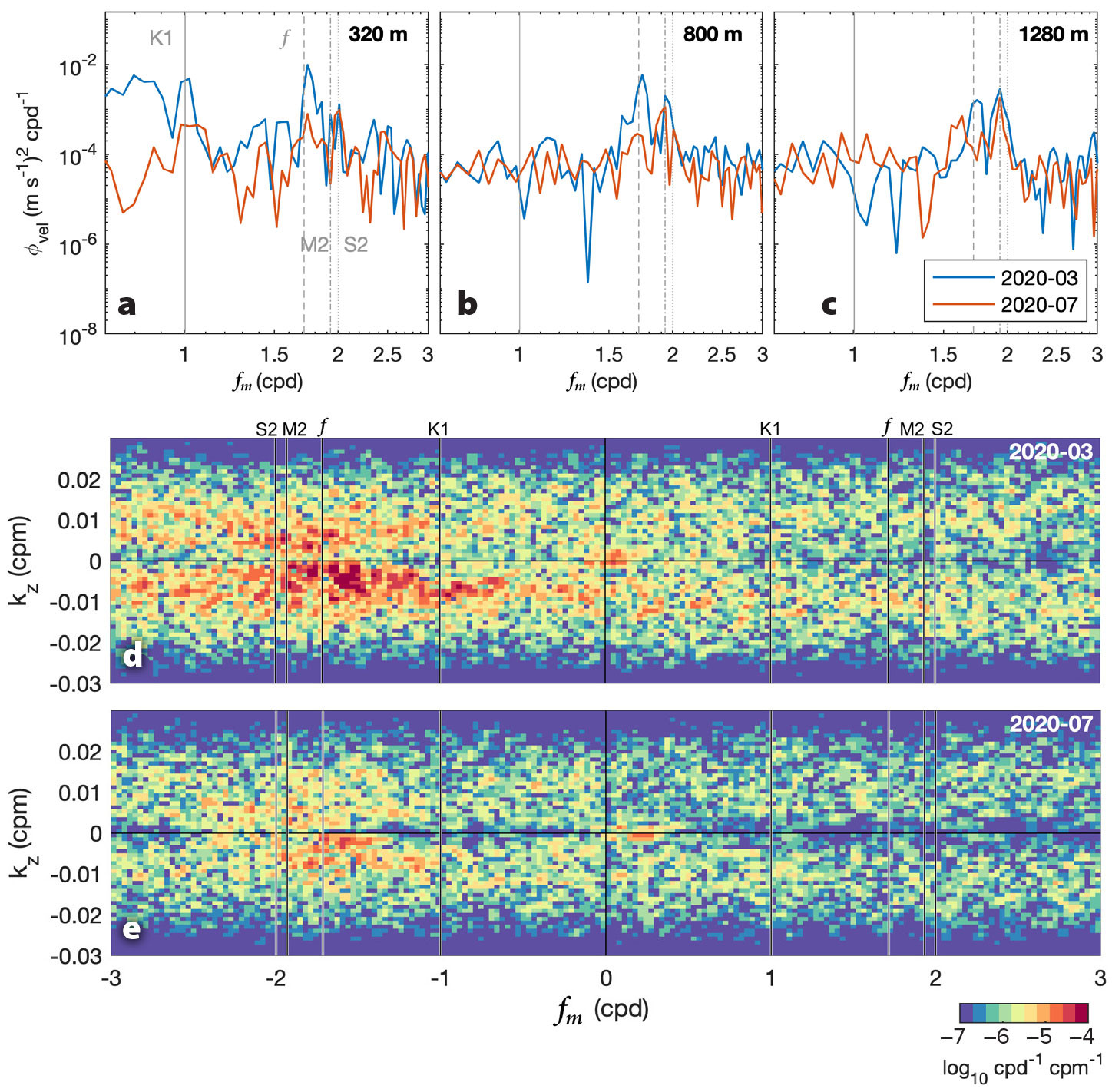
FIGURE 5. (a–c) Power spectra of buoyancy-normalized velocity at 320, 800, and 1,280 m depths with differing background and forcing conditions. The first (blue lines) is during the enhanced KENI event of March 2020 associated with a deep mixed-layer depth and negative vorticity. The second event (red lines) is during a period with shallow mixed-layer depth, positive vorticity, and decreased wind-stress in July 2020. Local inertial (f), semidiurnal (M2), and diurnal (K1) frequencies are marked with dashed, dotted, and solid gray vertical lines, respectively. (d,e) Two-dimensional wavenumber-​frequency spectra of buoyancy-normalized shear (uz + ivz) from the same two subsets: (d) March and (e) July 2020. Local inertial (f) semidiurnal (M2 and S2), and diurnal (K1) frequencies are indicated with solid vertical lines. > High res figure

 

In summer, when winds are reduced and the mixed layer is thinner, the semi­diurnal tidal peak dominates at all depths and is similar to the spectral content at Reykjanes Ridge to the west (Vic et al., 2021). The M₂ peak is more prominent at 1,280 m than 320 m depth (Figure 5a,c). While the inertial peak is smaller, a blue shift is still evident where the peak is shifted toward higher frequency.

As an additional step to assess seasonal variability of spectral content of shear, a two-dimensional (2D) wavenumber-​frequency spectrum is computed (e.g., Pinkel, 2008; Fer, 2014) in order to consider patterns of variability in both time and space simultaneously. The sign of phase propagation is given by the relative signs of frequency, f_m, and vertical wavenumber, k_z. For freely propagating linear internal waves, downward-​propagating energy (upward-propagating phase) corresponds to f_m/k_z > 0, whereas upward-​propagating energy is in quadrants with f_m/k_z < 0. Wind-generated downward near-inertial energy is expected in the lower-left quadrant (f_m < 0 and k_z < 0).

During winter, the 2D spectrum is dominated by a peak in the bottom left quadrant (Figure 5d), consistent with downward-​propagating near-​inertial waves forced by winds. The near-​inertial peak spreads toward both higher and lower frequencies with increasing wave­number k_z. This is consistent with smearing associated with Doppler shifting due to internal-​wave vertical velocities with increasing vertical wavenumbers (Holloway, 1983; Sherman and Pinkel, 1991; Pinkel, 2014). A smaller peak appears at the M₂ semidiurnal frequency in both positive and negative wavenumber bands at approximately k_z = 0.0059 cpm (170 m wavelength). The right-hand side of the 2D spectrum contains relatively weak signals, indicating mostly clockwise rotation of shear with time, as is expected in the Northern Hemisphere.

During summer, there is a similar peak in both positive and negative wave­numbers at the M₂ semidiurnal frequency and a near-inertial peak in the bottom left quadrant from k_z = 0 to −0.01 cpm. Again, the peak at the local inertial frequency (f) spreads with increasing vertical wavenumber towards both higher and lower frequencies, consistent with Doppler shifting.

 

Vorticity Influence on Directionality of Vertical Shear

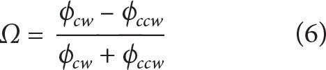
Following Leaman and Sanford (1975), upward and downward energy propagation can be diagnosed by separating Northern Hemisphere shear profiles into counterclockwise-(CCW) and clockwise-(CW) with-depth components. Following Waterhouse et al. (2022), rotary-​with-​depth spectra are calculated from buoyancy-normalized vertical shear for each gridded 10 min sample to obtain CCW- and CW-with-depth rotary shear components. CCW and CW shear variances, ϕ_ccw and ϕ_cw, are calculated by integrating over 32–832 m vertical wavelengths and normalizing by the buoyancy-normalized GM76 shear spectrum (Garrett and Munk, 1975) integrated over the same wavenumber range.

The non-dimensional vertical asymmetry ratio,

(Gonella, 1972; Waterhouse et al., 2022), describes the relative dominance of downward- vs. upward-propagating shear variance in the Northern Hemisphere.

From May 2019 to October 2020, one-day-​smoothed Ω indicates enhanced down-​going energy during winter (Figure 6a), in line with the expectation that wind-generated NIWs are passing through the observational array. Probability distributions indicate enhanced downward-propagating shear during winter (_winter = 0.10) and near-equal directionality during summer (_summer = 0.03; Figure 6b). The winter average is close to the 200–600 m average (0.13) from a global compendium of shear observations (Waterhouse et al., 2022).

To determine the influence of background vorticity on the preferred direction of vertical energy propagation, daily-​filtered Ω is compared to background vorticity using a bivariate histogram (Figure 6c). Results suggest that downward propagation is particularly dominant within negative vorticity, consistent with historical observations that have shown trapping of inertial signals within anticyclonic eddies (e.g., Kunze, 1986; Kunze et al.,1995; Joyce et al., 2013; Essink et al., 2022). Even in weak normalized vorticity (|ζ/f | < 0.1), there is enhanced downward- compared to upward-​propagating shear variance within anticyclonic vorticity.

 

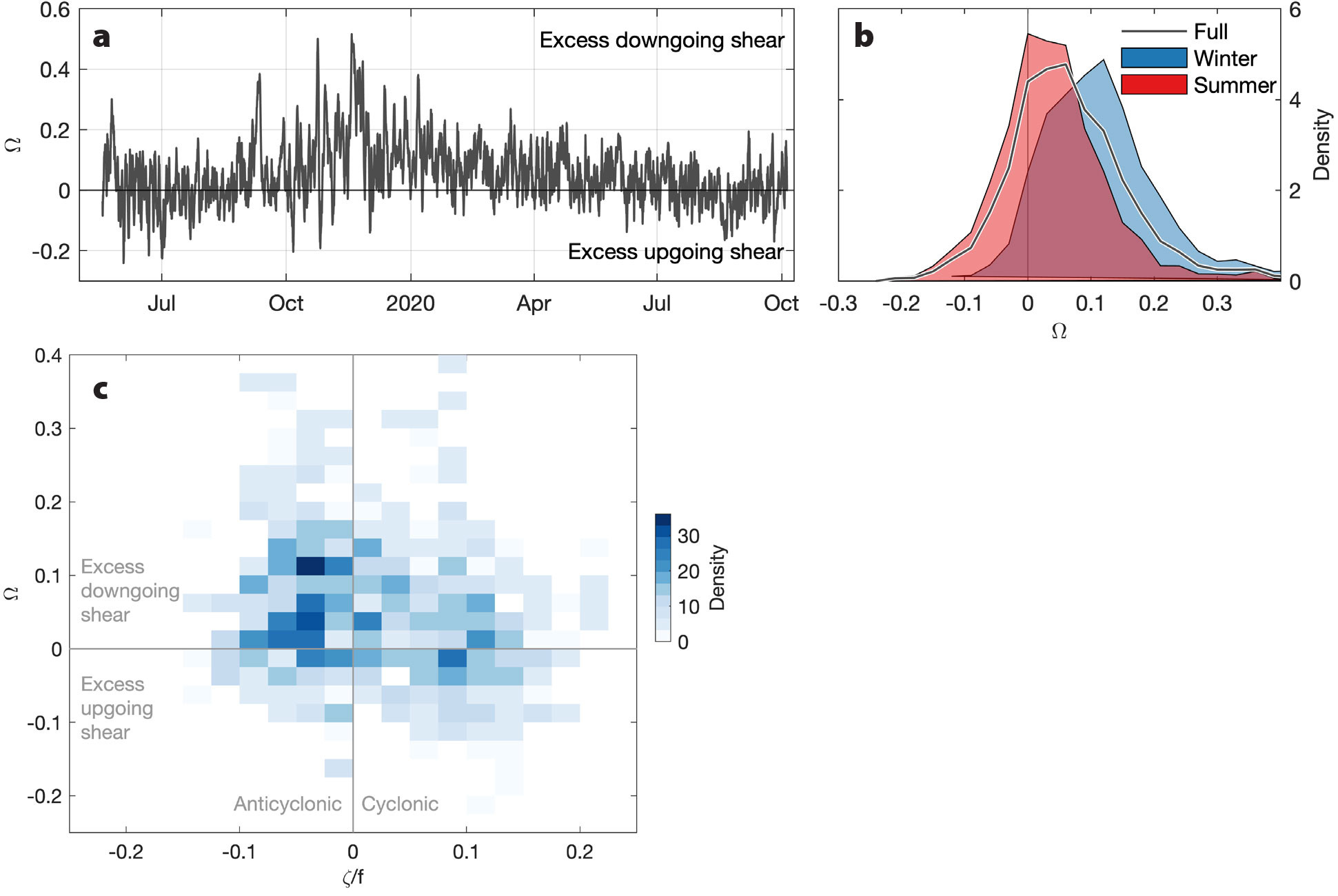
FIGURE 6. (a) Time series of asymmetry ratio, Ω, calculated from buoyancy-normalized rotary shear based on moored current meter observations. Ω is smoothed using a one-day third-order median filter. (b) Probability density function of median-filtered Ω over the full mooring record from May 2019 to October 2020 (black), winter (blue; November 1, 2019, to April 30, 2020), and summer (red; May–October 2019 and May–October 2020). (c) Bivariate histogram of Ω and normalized vorticity, ζ/f, for the full observational period at NISKINe mooring M1. Left and right halves of the plot indicate anticyclonic and cyclonic vorticity. Top and bottom halves show excess downward- and upward-propagating shear. > High res figure

 

 

 

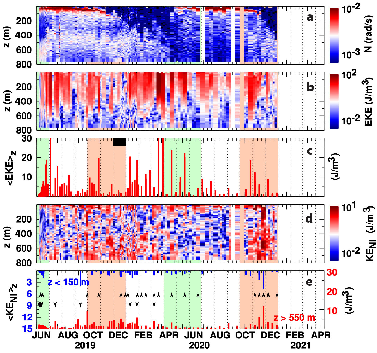
FIGURE 7. EM-APEX profiling float profile time-series of (a) buoyancy frequency N, (b) subinertial eddy horizontal kinetic energy (EKE) as a function of depth, and (c) depth-averaged EKE. (d) Near-inertial/semidiurnal kinetic energy (KENI) as a function of depth. (e) Depth-averaged KENI in the upper 150 m (blue bars and left axis) and in the permanent pycnocline over 550–800 m depth (red bars and right axis). Light green shading denotes spring and rose shading autumn. The black bar along the upper axis in (c) marks the interval when the float was crossing the Reykjanes Ridge (Figure 1). Down and up arrows in (e) mark profiles with clear clockwise-with-depth (downgoing energy) or counterclockwise-with-depth (upgoing energy) signatures. > High res figure

 

Seasonality and Lateral Variability of Low-Mode Near-Inertial Energy Flux

Internal wave radiation transports energy from generation sites across ocean basins (Nash et al., 2005). Near-inertial energy flux is the flux of energy associated with waves close to the inertial frequency. Typically, low-mode near-inertial waves propagate rapidly from generation sites unless they are vorticity-trapped. Higher modes have much slower propagation speeds and thus generally do not contribute significantly to lateral energy fluxes. We determine the near-inertial low-mode energy flux at NISKINe mooring M1 and at OSNAP mooring MM4 ~100 km to the south (Gill, 1984; Kunze et al., 2002; Alford, 2003b; Althaus et al., 2003).

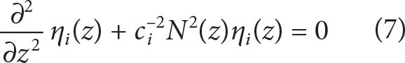
Low-mode vertical structure is determined by the stratification of the water column N(z). For hydrostatic waves (ω << N), the modes are solutions to

with vertical displacement of water parcels η where c_i is the eigenspeed of mode i. Boundary conditions in their simplest form are η(0) = η(H) = 0 (i.e., a rigid lid at the top and a flat bottom). Determining orthogonal modes with a free ocean surface is also possible (Kelly, 2016). Vertical modes for horizontal velocities can then be determined from the internal-wave polarization relations. Seasonal evolution of mode-1 shapes at the NISKINe mooring is shown in Figure 2e.

Time series of vertical displacement are estimated from moored temperature observations and seasonally resolved climatological temperature gradients (WOCE-Argo; Gouretski, 2019) as

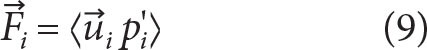
at discrete depths z_j. Modal profiles of near-inertial velocity, _i(z,t), and displacement, η_i(z,t), for the three lowest baroclinic modes are determined by projecting mode shapes onto near-inertial band-pass-filtered time-series _j(z,t) and η_j(z, t) via a least-squares inverse at each time t. Figure 8a,b shows an example of mode-shape projection and reconstruction of velocity and displacement estimates using the three lowest baroclinic modes for one time step. From displacement modes, modal baroclinic pressure perturbations p_i' are the depth integral of N²η_i(z) minus the depth mean (Kunze et al., 2002). Near-inertial horizontal energy-flux  per mode i is

where angle brackets indicate averaging over a wave period.

 

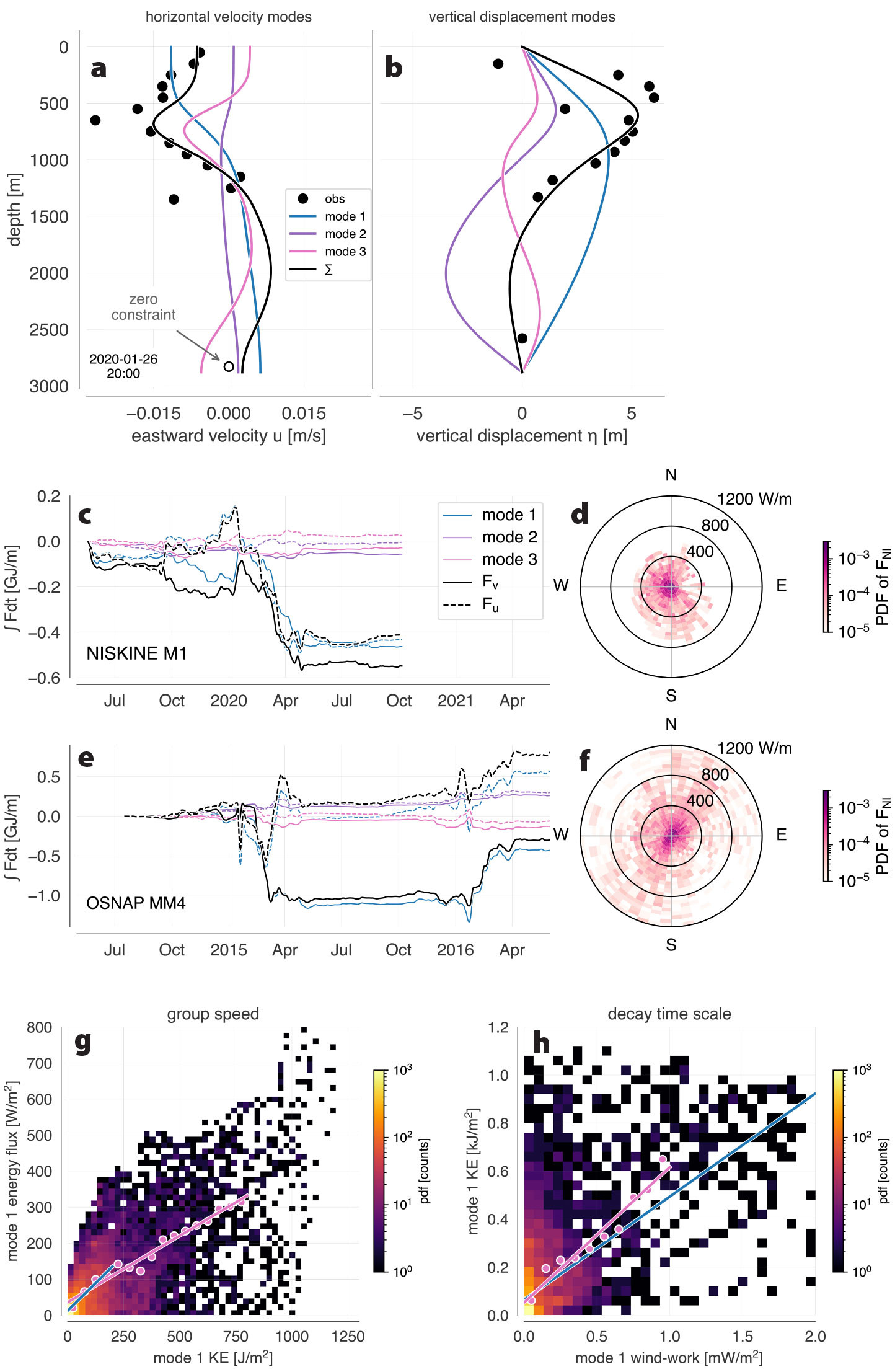
FIGURE 8. Low-mode near-inertial wave properties. (a,b) Example horizontal velocity and vertical displacement projections. In (a,b), measurements (black dots) are from January 26, 2020, at 20:00. The open circle shows zero horizontal velocity constraint applied near the bottom. Colored lines show the results of a least squares fit of the three gravest baroclinic modes to eastward velocity and vertical displacement. Black curves show the sum of these first three modes. (c–f) Energy fluxes at NISKINe mooring M1 (c,d) and OSNAP mooring MM4 (e,f). Panels c and e show the cumulative integral in time of depth-integrated low-mode near-inertial energy flux. Colored lines show energy-flux contributions from modes 1 to 3, black lines the sum over the three modes. Dashed lines show east-west components, solid lines north-south components. Note different scales on the y-axes in c and e. Times in c and e on the x-axes also differ but have been aligned to match seasonally. Middle right panels (d,f) show histograms of flux magnitude and direction at both sites. (g) Group speed, obtained by regressing energy flux onto kinetic energy content, is 0.6 m s–1 (slope of fit) for kinetic energy less than 200 J m–2 where the majority of the data reside (blue line). Using a larger data range up to 800 J m–2, group speed is 0.4 m s–1 (pink line). (h) Replenishment time scale from regressing kinetic energy content onto near-inertial wind-work. Energy decay time is 5 days from a fit to all data (blue) and 6.5 days from a fit to binned data for wind-work smaller than 1 mW m–2. > High res figure

 

Mode projections were complicated at NISKINe mooring M1 because velocity measurements near the bottom terminated after one week due to instrument failure. The first week of data near the bottom shows near-inertial velocities to be less than 1 cm s^–1. A comparison of flux calculations for this first week assuming zero velocity at depth as compared to the measured velocity (see open circle in Figure 8a) shows a difference of less than 5% in energy flux. Therefore, to constrain horizontal velocity modes at depth, we assumed zero near-inertial velocities near the bottom throughout the time series.

Low-mode near-inertial energy fluxes exhibit a distinct seasonal cycle at both NISKINe and OSNAP mooring sites (Figure 8c–f). Most of the energy flux is in mode 1, and the strongest low-mode NI fluxes occur between January and April at both sites. Low-mode fluxes thus appear to correlate not only with increased winter near-inertial wind-work but also possibly with mixed-layer depth (Figure 4). Simmons and Alford (2012) discuss how a deeper winter mixed layer may lead to stronger forcing of low modes as the mixed layer projects better onto low-mode shapes.

Low-mode energy-flux magnitudes (summed over the first three modes) at the NISKINe mooring are 74 W m^–1 on average, a factor of two smaller than those at the OSNAP site (174 W m^–1). Similarly, the 95 percentile of low-mode near-​inertial energy-flux is 305 W m^–1 at NISKINe and 774 W m^–1 at OSNAP. These are within the range of annual near-inertial energy fluxes from western boundaries subject to enhanced wind input (100 W m^–1) and below those from the Southeast Pacific and the Southern Ocean (between 300 W m^–1 and 500 W m^–1), where wind input is large (Raja et al., 2022).

Local near-inertial wind-work alone does not explain the difference in magnitude because the seasonal cumulative near-inertial wind forcing is O(3) kJ m^–2 at both sites. Although these two data sets are not contemporaneous, equivalent surface forcing provides a qualitative estimate of the lateral variability in low-mode energy fluxes. An accumulation of near-inertial energy flux propagating from elsewhere or focused by mesoscale eddies may explain the higher energy flux at OSNAP (see Summary and Discussion). Integrated over one season, the low-mode near-inertial energy flux is directed to the southwest at the NISKINe site, though the strongest flux events are directed to the southeast. Flux direction differs between the two seasons at OSNAP with the 2014/2015 flux southward while the 2015/2016 flux was northwestward on average. The average meridional vorticity gradient north of the OSNAP site at O(100) km scale was negative between January and March 2016 when northward low-mode flux was strongest. The meridional relative vorticity gradient amplitude at this time was two orders of magnitude larger than the local change in planetary meridional inertial frequency gradient, indicating that local mesoscale conditions would have counteracted the effect of a varying Coriolis frequency with latitude.

Fluxes to the southwest are negligible at the OSNAP mooring site. This may indicate an influence of Hatton Bank, a region of much shallower bathymetry extending approximately from southwest to northeast (Figure 1), on low-mode near-​inertial wave propagation. This is at odds with expected reflection behavior from a slope (Eriksen, 1982) but is consistent with a topographically trapped wave. The physical mechanisms for topographic trapping, however, are unclear and warrant further investigation.

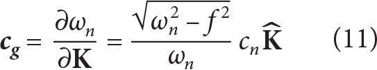
Mode-1 wave properties at the NISKINe mooring are estimated from mode-1 eigenspeed c₁ and the internal-​wave dispersion relation (e.g., Alford and Zhao, 2007):

where ω_n = mode-n frequency, c_n = mode-n eigenspeed, and K = (k_x, k_y) horizontal wavevector. Horizontal mode group speed is

where  points in the direction of horizontal wave propagation. c_g is estimated via regression of mode-1 energy flux onto mode-1 kinetic energy content (Figure 8g). Depending on the range of data used in the regression, mode-1 group speed is between 0.4 and 0.6 m s^–1, with the higher estimate stemming from rejecting large-amplitude energy content and fluxes. Taking an average mode-1 group speed, c_g = 0.5 m s^–1, Equation 11 predicts a characteristic mode-1 frequency ω₁ = 1.055f. Upper and lower frequency bounds based on 0.6 m s^–1 > c_g > 0.4 m s^–1 are 1.078f and 1.035f. Horizontal wave­number magnitude is 2.7 × 10^–5 m^–1, corresponding to a characteristic horizontal wavelength of ~230 km for the lowest-mode near-inertial waves.

 

Summary and Discussion

Observations from an 18-month deployment of a moored array in Iceland Basin as part of the NISKINe project captured variability in near-inertial wave generation and propagation associated with seasonality of surface wind forcing and heat loss that peak in winter, and the background eddy field that peaks in summer.

While mean currents show little depth dependence in the upper 1,500 m, inertially band-passed velocities are strongly depth-dependent (Figure 4). Near-inertial kinetic energy in the upper 1,500 m follows the seasonal cycle in wind-work, so it is enhanced during winter. Overall, near-inertial kinetic energy in winter scales with seasonal pycnocline depth. Depth penetration of near-​inertial kinetic energy below the mixed-layer depth is linked to vorticity and mostly independent of mixed-layer depth.

The spectral content of velocity and vertical shear indicate a peak in the local inertial band during winter. The peak in the inertial band is just above the local inertial frequency due either to near-​inertial waves propagating from further north (Gill, 1984) or modification of near-inertial wave generation by the background mesoscale eddy vorticity field (Weller, 1982).

Following a typical winter storm, vertical shear is predominantly downgoing, particularly in anticyclonic background vorticity. Anticyclonic eddies act as inertial drainpipes (e.g., Kunze, 1985; Kunze et al., 1995; Vic et al., 2021; Yu et al., 2022; Thomas et al., 2023) where near-​inertial wave energy is focused, trapped, and amplified (Kunze, 1986; Kunze et al., 1995; Lelong et al., 2020; Essink et al., 2022).

Near-inertial energy in the lowest baroclinic modes propagates south on average. It is larger and more variable at the OSNAP site where its propagation direction is aligned with the sharp bathymetry gradient of Hatton Bank to the east. At both NISKINe and OSNAP sites, low-mode energy-flux magnitudes increase when the mixed-layer depth better matches the zero crossing of the gravest baroclinic horizontal velocity mode (compare Figures 2e and 3d).

Mode-1 wave properties indicate basin-​scale forcing of low-mode near-​inertial energy fluxes at the NISKINe mooring. A flux of energy from the north is necessary to close a local energy budget. The extent of the forcing region may be estimated under the assumption that all near-inertial wind-work excites low-mode near-inertial waves. Annual mean low-mode near-inertial energy-flux at the NISKINe site is 74 W m^–1. Division by annual mean near-inertial wind-work of 0.12 mW m^–2 yields an upstream forcing region of about 600 km. Because ERA5 reanalysis winds underestimate wind power at the NISKINe site by about 40% due to inadequate temporal resolution (Klenz et al., 2022), the forcing region may scale down to about 360 km, or the northern extent of Iceland Basin. Mode-1 group speeds of about 0.5 m s^–1 indicate rapid lateral progression of near-inertial waves. At this speed, a low-mode near-​inertial wave with 230 km characteristic lateral extent passes through the mooring site in about five days. A similar replenishment time­scale is estimated by regressing mode-1 energy content onto near-​inertial wind-work (Figure 8h); initial northward propagation of low-mode near-inertial waves is possible, contributing to the relatively wide spread in estimates for group velocity and replenishment time scale in Figure 8g,h. At the characteristic mode-1 frequency ω₁ = 1.055f, the northward distance to the turning latitude based on the local change in inertial frequency β is (ω₁ – f) / β = 586 km. Waves at ω₁ are thus free to propagate in the full northward range of Iceland Basin.

 

Acknowledgments

This study was carried out through funding from the Office of Naval Research grants for GV and AFW under N00014-18-1-2423 and N00014-22-1-2182. HLS and TK were supported under ONR grant N00014-18-1-2386. EK, CBW, RCL, and JBG were supported under N00014-18-1-2598. SMK was supported under N00014-18-1-2800. JNM was supported under N00014-18-1-2788. JAM was supported under N00014-18-1-2388. We thank captains Derek Bergeron and Kent Sheasley and the whole crew of R/V Neil Armstrong for outstanding support of our science operations at sea in 2019 and 2020. We are grateful for UNOLS, ONR, and NSF, making a safe joint OSNAP/NISKINe mooring recovery cruise possible during the early days of the COVID-19 pandemic. We would like to thank Clement Vic and an anonymous reviewer for their helpful and thoughtful comments, which greatly improved the final version of the manuscript.

Data Availability Statement

Mooring data collected during NISKINe are available from the authors upon request. This study has been conducted using EU Copernicus Marine Service Information: Altimeter satellite gridded sea level anomalies and derived geostrophic currents (https://doi.org/​10.48670/moi-00148); sea surface temperature (Merchant et al., 2019, https://doi.org/​10.48670/moi–00169). Wind data from ERA5 reanalysis (Hersbach et al., 2023) is available for download at https://doi.org/10.24381/cds.bd0915c6. The WOCE/Argo Global Hydrographic Climatology (Gouretski, 2018) is available at https://doi.org/10.1594/WDCC/WAGHC_V1.0. The Argo MLD climatology (Holte et al., 2017) is available at http://mixedlayer.ucsd.edu. OSNAP mooring data (Johns and Houk, 2018) are available at https://doi.org/10.7924/r42n52w51.

Voet, G., A.F. Waterhouse, A. Savage, E. Kunze, J.A. MacKinnon, M.H. Alford, J.A. Colosi, H.L. Simmons, T. Klenz, S.M. Kelly, J.N. Moum, C.B. Whalen, R.-C. Lien, and J.B. Girton. 2024. Near-inertial energy variability in a strong mesoscale eddy field in the Iceland Basin. Oceanography, https://doi.org/10.5670/oceanog.2024.302.

Alford, M.H. 2003a. Redistribution of energy available for ocean mixing by long-range propagation of internal waves. Nature 423(6936):159–162, https://doi.org/​10.1038/nature01628.

Alford, M.H. 2003b. Improved global maps and 54-year history of wind-work on ocean inertial motions. Geophysical Research Letters 30(8), https://doi.org/10.1029/2002GL016614.

Alford, M.H., and Z. Zhao. 2007. Global patterns of low-mode internal-wave propagation: Part II. Group velocity. Journal of Physical Oceanography 37(7):1,849–1,858, https://doi.org/​10.1175/JPO3086.1.

Alford, M.H., A.Y. Shcherbina, and M.C. Gregg. 2013. Observations of near-inertial internal gravity waves radiating from a frontal jet. Journal of Physical Oceanography 43(6):1,225–1,239, https://doi.org/​10.1175/JPO-D-12-0146.1.

Alford, M.H., J.A. MacKinnon, R. Pinkel, and J.M. Klymak. 2017. Space-time scales of shear in the North Pacific. Journal of Physical Oceanography 47(10):2,455–2,478, https://doi.org/​10.1175/JPO-D-17-0087.1.

Alford, M.H. 2020. Revisiting near-inertial wind work: Slab models, relative stress, and mixed layer deepening. Journal of Physical Oceanography 50(11):3,141–3,156, https://doi.org/​10.1175/jpo-d-20-0105.1.

Althaus, A.M., E. Kunze, and T.B. Sanford. 2003. Internal tide radiation from Mendocino Escarpment. Journal of Physical Oceanography 33(7):1,510–1,527, https://doi.org/​10.1175/​1520-​0485​(2003)​033​<1510:​ITRFME>​2.0.CO;2.

Asselin, O., and W.R. Young. 2020. Penetration of wind-generated near-inertial waves into a turbulent ocean. Journal of Physical Oceanography 50(6):1,699–1,716, https://doi.org/​10.1175/JPO-D-19-0319.1.

Bühler, O., and M.E. McIntyre. 2005. Wave capture and wave-vortex duality. Journal of Fluid Mechanics 534:67–95, https://doi.org/10.1017/S0022112005004374.

Chelton, D.B., M.G. Schlax, R.M. Samelson, J.T. Farrar, M.J. Molemaker, J.C. McWilliams, and J. Gula. 2019. Prospects for future satellite estimation of small-scale variability of ocean surface velocity and vorticity. Progress in Oceanography 173:256–350, https://doi.org/https://doi.org/10.1016/j.pocean.​2018.10.012.

D’Asaro, E.A., and H. Perkins. 1984. A near-​inertial internal wave spectrum for the Sargasso Sea in late summer. Journal of Physical Oceanography 14(3):489–505, https://doi.org/​10.1175/​1520-​0485​(1984)​014​<0489:ANIIWS>​2.0.CO;2.

D’Asaro, E.A. 1985. The energy flux from the wind to near-inertial motions in the surface mixed layer. Journal of Physical Oceanography 15(8):1,043–1,059, https://doi.org/​10.1175/​1520-​0485​(1985)015​<1043:TEFFTW>​2.0.CO;2.

D’Asaro, E.A., C.C. Eriksen, M.D. Levine, C.A. Paulson, P. Niiler, and Pim Van Meurs. 1995. Upper-ocean inertial currents forced by a strong storm: Part I. Data and comparisons with linear theory. Journal of Physical Oceanography 25(11):2,909–2,936, https://doi.org/10.1175/1520-0485(1995)025<2909:UOICFB>2.0.CO;2.

de Lavergne, C., C. Vic, G. Madec, F. Roquet, A.F. Waterhouse, C.B. Whalen, Y. Cuypers, P. Bouruet-Aubertot, B. Ferron, and T. Hibiya. 2020. A parameterization of local and remote tidal mixing. Journal of Advances in Modeling Earth Systems 12(5):e2020MS002065, https://doi.org/​10.1029/2020ms002065.

Elipot, S., R. Lumpkin, and G. Prieto. 2010. Modification of inertial oscillations by the mesoscale eddy field. Journal of Geophysical Research: Oceans 115(C9), https://doi.org/​10.1029/2009JC005679.

Eriksen, C.C. 1982. Observations of internal wave reflection off sloping bottoms. Journal of Geophysical Research: Oceans 87(C1):525–538, https://doi.org/10.1029/JC087iC01p00525.

Essink, S., E. Kunze, R.-C. Lien, R. Inoue, and S.-i. Ito. 2022. Near-inertial wave interactions and turbulence production in a Kuroshio anticyclonic eddy. Journal of Physical Oceanography 52(11):2,687–2,704, https://doi.org/10.1175/JPO-D-21-0278.1.

Fer, I. 2014. Near-inertial mixing in the Central Arctic Ocean. Journal of Physical Oceanography 44(8):2,031–2,049, https://doi.org/​10.1175/JPO-D-13-0133.1.

Fu, L.-L. 1981. Observations and models of inertial waves in the deep ocean. Reviews of Geophysics 19(1):141–170, https://doi.org/10.1029/RG019i001p00141.

Garrett, C., and W. Munk. 1975. Space-time scales of internal waves: A progress report. Journal of Geophysical Research 80(3):291–298, https://doi.org/​10.1029/JC080i003p00291.

Garrett, C., and W. Munk. 1979. Internal waves in the ocean. Annual Review of Fluid Mechanics 11(1):339–369, https://doi.org/10.1146/annurev.fl.11.010179.002011.

Garrett, C. 2001. What is the ‘near-inertial’ band and why is it different from the rest of the internal wave spectrum? Journal of Physical Oceanography 31(4):962–971, https://doi.org/​10.1175/​1520-0485(2001)031​<0962:witnib>​2.0.co;2.

Gill, A.E. 1984. On the behavior of internal waves in the wakes of storms. Journal of Physical Oceanography 14(7):1,129–1,151, https://doi.org/​10.1175/​1520-0485​(1984)014​<1129:OTBOIW>​2.0.CO;2.

Girton, J.B., C.B. Whalen, R.-C. Lien, and E. Kunze. 2024. Coherent float arrays for near-inertial wave studies. Oceanography, in press.

Gonella, J. 1972. A rotary-component method for analysing meteorological and oceanographic vector time series. Deep Sea Research 19:833–846, https://doi.org/10.1016/0011-7471(72)90002-2.

Gouretski, V. 2018. WOCE-Argo global hydrographic climatology (WAGHC Version 1.0). World Data Center for Climate (WDCC) at DKRZ, https://doi.org/​10.1594/​WDCC/WAGHC_V1.0.

Gouretski, V. 2019. A new global ocean hydrographic climatology. Atmospheric and Oceanic Science Letters 12(3):226–229, https://doi.org/10.1080/​16742834.​2019.1588066.

Gregg, M.C. 1989. Scaling turbulent dissipation in the thermocline. Journal of Geophysical Research: Oceans 94(C7):9,686–9,698, https://doi.org/​10.1029/​JC094iC07p09686.

Halle, C., and R. Pinkel. 2003. Internal wave variability in the Beaufort Sea during the winter of 1993/1994. Journal of Geophysical Research: Oceans 108(C7), https://doi.org/10.1029/2000JC000703.

Henyey, F.S., J. Wright, and S.M. Flatte. 1986. Energy and action flow through the internal wave field: An eikonal approach. Journal of Geophysical Research 91:8,487–8,495, https://doi.org/10.1029/JC091iC07p08487.

Hersbach, H., B. Bell, P. Berrisford, G. Biavati, A. Horányi, J. Muñoz Sabater, J. Nicolas, C. Peubey, R. Radu, I. Rozum, and others. 2023. ERA5 hourly data on pressure levels from 1940 to present. Copernicus Climate Change Service (C3S) Climate Data Store (CDS), https://doi.org/10.24381/cds.bd0915c6.

Holloway, G. 1983. A conjecture relating oceanic internal waves and small-scale processes. Atmosphere-Ocean 21 (1):107–122, https://doi.org/​10.1080/07055900.1983.9649159.

Holte, J., L.D. Talley, J. Gilson, and D. Roemmich. 2017. An Argo mixed layer climatology and database. Geophysical Research Letters 44(11):5,618–5,626, https://doi.org/10.1002/2017GL073426.

Jochum, M., B.P. Briegleb, and G. Danabasoglu. 2013. The impact of oceanic near-inertial waves on climate. Journal of Climate 26(9):2,833–2,844, https://doi.org/10.1175/JCLI-D-12-00181.1.

Johns, W., and A. Houk. 2018. Microcat, current meter and ADCP data from the eastern mid-Atlantic ridge mooring array as part of OSNAP (Overturning in the Subpolar North Atlantic Program). Duke Digital Repository, https://doi.org/https://doi.org/10.7924/r42n52w51.

Joyce, T.M., J.M. Toole, P. Klein, and L.N. Thomas. 2013. A near-inertial mode observed within a Gulf Stream warm-core ring. Journal of Geophysical Research: Oceans 118(4):1,797–1,806, https://doi.org/10.1002/jgrc.20141.

Kara, A.B., P.A. Rochford, and H.E. Hurlburt. 2000. An optimal definition for ocean mixed layer depth. Journal of Geophysical Research: Oceans 105(C7):16,803–16,821, https://doi.org/​10.1029/2000JC900072.

Kelly, K.A., and L. Thompson. 2002. Scatterometer winds explain damped Rossby waves. Geophysical Research Letters 29(20):52-1–52-4, https://doi.org/​10.1029/2002GL015595.

Kelly, S.M. 2016. The vertical mode decomposition of surface and internal tides in the presence of a free surface and arbitrary topography. Journal of Physical Oceanography 46(12):3,777–3,788, https://doi.org/10.1175/JPO-D-16-0131.1.

Klenz, T., H.L. Simmons, L. Centurioni, J.M. Lilly, J.J. Early, and V. Hormann. 2022. Estimates of near-inertial wind power input using novel in situ wind measurements from Minimet surface drifters in the Iceland Basin. Journal of Physical Oceanography 52(10):2,417–2,430, https://doi.org/​10.1175/jpo-d-21-0283.1.

Kunze, E., and T.B. Sanford. 1984. Observations of near-inertial waves in a front. Journal of Physical Oceanography 14(3):566–581, https://doi.org/​10.1175/​1520-0485(1984)014​<0566:OONIWI>​2.0.CO;2.

Kunze, E. 1985. Near-inertial wave propagation in geostrophic shear. Journal of Physical Oceanography 15(5):544–565, https://doi.org/​10.1175/​1520-0485​(1985)015​<0544:NIWPIG>​2.0.CO;2.

Kunze, E. 1986. The mean and near-inertial velocity fields in a warm-core ring. Journal of Physical Oceanography 16(8):1,444–1,461, https://doi.org/​10.1175/1520-0485(1986)016<1444:TMANIV>​2.0.CO;2.

Kunze, E., A.J. Williams, and M.G. Briscoe. 1990. Observations of shear and vertical stability from a neutrally buoyant float. Journal of Geophysical Research 95(C10):18,127–18,142, https://doi.org/​10.1029/JC095iC10p18127.

Kunze, E., R.W. Schmitt, and J.M. Toole. 1995. The energy balance in a warm-core ring’s near-​inertial critical layer. Journal of Physical Oceanography 25(5):942–957, https://doi.org/​10.1175/​1520-​0485​(1995)​025​<0942:​TEBIAW>​2.0.CO;2.

Kunze, E., L.K. Rosenfeld, G.S. Carter, and M.C. Gregg. 2002. Internal waves in Monterey Submarine Canyon. Journal of Physical Oceanography 32(6):1,890–1,913, https://doi.org/​10.1175/1520-0485(2002)032<1890:IWIMSC>​2.0.CO;2.

Kunze, E. 2017a. Internal-wave-driven mixing: Global geography and budgets. Journal of Physical Oceanography 47(6):1,325–1,345, https://doi.org/​10.1175/jpo-d-16-0141.1.

Kunze, E. 2017b. The internal-wave-driven meridional overturning circulation. Journal of Physical Oceanography 47(11):2,673–2,689, https://doi.org/​10.1175/jpo-d-16-0142.1.

Kunze, E., R.-C. Lien, C.B. Whalen, J.B. Girton, B. Ma, and M.C. Buijsman. 2023. Seasonal variability of near-inertial/semidiurnal fluctuations and turbulence in the sub-Arctic North Atlantic. Journal of Physical Oceanography 53(12):2,717–2,735, https://doi.org/10.1175/JPO-D-22-0231.1.

Leaman, K.D., and T.B. Sanford. 1975. Vertical energy propagation of inertial waves: A vector spectral analysis of velocity profiles. Journal of Geophysical Research 80(15):1,975–1,978, https://doi.org/10.1029/JC080i015p01975.

Le Boyer, A., and M.H. Alford. 2021. Variability and sources of the internal wave continuum examined from global moored velocity records. Journal of Physical Oceanography 51(9):2,807–2,823, https://doi.org/10.1175/JPO-D-20-0155.1.

Lee, D.-K., and P.P. Niiler. 1998. The inertial chimney: The near-inertial energy drainage from the ocean surface to the deep layer. Journal of Geophysical Research: Oceans 103(C4):7,579–7,591, https://doi.org/​10.1029/97JC03200.

Lelong, M.-P., Y. Cuypers, and P. Bouruet-Aubertot. 2020. Near-inertial energy propagation inside a Mediterranean anticyclonic eddy. Journal of Physical Oceanography 50(8):2,271–2,288, https://doi.org/10.1175/JPO-D-19-0211.1.

Lien, R.-C., and P. Müller. 1992. Consistency relations for gravity and vortical modes in the ocean. Deep Sea Research Part A 39(9):1,595–1,612, https://doi.org/​10.1016/​0198-0149(92)90050-4.

Lien, R.-C., and T.B. Sanford. 2019. Small-scale potential vorticity in the upper-ocean thermocline. Journal of Physical Oceanography 49(7):1,845–1,872, https://doi.org/10.1175/JPO-D-18-0052.1.

Lozier, M.S., F. Li, S. Bacon, F. Bahr, A.S. Bower, S.A. Cunningham, M.F. de Jong, L. de Steur, B. deYoung, J. Fischer, and others. 2019. A sea change in our view of overturning in the subpolar North Atlantic. Science 363(6426):516–521, https://doi.org/10.1126/science.aau6592.

Martin, A.P., I.P. Wade, K.J. Richards, and K.J. Heywood. 1998. The PRIME eddy. Journal of Marine Research 56(2):439–462.

McComas, C.H., and F.P. Bretherton. 1977. Resonant interaction of oceanic internal waves. Journal of Geophysical Research 82(9):1,397–1,412, https://doi.org/​10.1029/JC082i009p01397.

McComas, C.H., and P. Müller. 2000. The dynamic balance of internal waves. Journal of Physical Oceanography 11(7):970–986, https://doi.org/​10.1175/​1520-0485(1981)011<0970:TDBOIW>​2.0.CO;2.

Merchant, C.J., O. Embury, C.E. Bulgin, T. Block, G.K. Corlett, E. Fiedler, S.A. Good, J. Mittaz, N.A. Rayner, D. Berry, and others. 2019. Satellite-based time-series of sea-surface temperature since 1981 for climate applications. Scientific Data 6(1):223, https://doi.org/10.1038/s41597-019-0236-x.

Moum, J.N., and J.D. Nash. 2009. Mixing measurements on an equatorial ocean mooring. Journal of Atmospheric and Oceanic Technology 26:317–336, https://doi.org/10.1175/2008JTECHO617.1.

Müller, P., D.J. Olbers, and J. Willebrand. 1978. The Iwex Spectrum. Journal of Geophysical Research: Oceans 83(C1):479–500, https://doi.org/10.1029/JC083iC01p00479.

Nash, J.D., M.H. Alford, and E. Kunze. 2005. Estimating internal wave energy fluxes in the ocean. Journal of Atmospheric and Oceanic Technology 22(10):1,551–1,570, https://doi.org/​10.1175/JTECH1784.1.

Naveira Garabato, A.C., X. Yu, J. Callies, R. Barkan, K.L. Polzin, E.E. Frajka-Williams, C.E. Buckingham, and S.M. Griffies. 2022. Kinetic energy transfers between mesoscale and submesoscale motions in the open ocean’s upper layers. Journal of Physical Oceanography 52(1):75–97, https://doi.org/10.1175/JPO-D-21-0099.1.

Park, J.-H., and D.R. Watts. 2005. Near-inertial oscillations interacting with mesoscale circulation in the southwestern Japan/East Sea. Geophysical Research Letters 32(10), https://doi.org/​10.1029/​2005GL022936.

Petit, T., H. Mercier, and V. Thierry. 2018. First direct estimates of volume and water mass transports across the Reykjanes Ridge. Journal of Geophysical Research: Oceans 123(9):6,703–6,719, https://doi.org/10.1029/2018JC013999.

Pinkel, R. 1985. A wavenumber-frequency spectrum of upper ocean shear. Journal of Physical Oceanography 15(11):1,453–1,469, https://doi.org/​10.1175/​1520-0485(1985)015<1453:AWFSOU>​2.0.CO;2.

Pinkel, R. 2008. The wavenumber-frequency spectrum of vortical and internal-wave shear in the western Arctic Ocean. Journal of Physical Oceanography 38(2):277–290, https://doi.org/​10.1175/2006JPO3558.1.

Pinkel, R. 2014. Vortical and internal wave shear and strain. Journal of Physical Oceanography 44(8):2,070–2,092, https://doi.org/​10.1175/JPO-D-13-090.1.

Rai, S., M. Hecht, M. Maltrud, and H. Aluie. 2021. Scale of oceanic eddy killing by wind from global satellite observations. Science Advances 7(28):eabf4920, https://doi.org/10.1126/sciadv.abf4920.

Rainville, L., and R. Pinkel. 2004. Observations of energetic high-wavenumber internal waves in the Kuroshio. Journal of Physical Oceanography 34(7):1,495–1,505, https://doi.org/​10.1175/1520-0485(2004)034<1495:OOEHIW>​2.0.CO;2.

Rainville, L., and R. Pinkel. 2006. Propagation of low-mode internal waves through the ocean. Journal of Physical Oceanography 36:1,220–1,236, https://doi.org/​10.1175/JPO2889.1.

Raja, K.J., M.C. Buijsman, J.F. Shriver, B.K. Arbic, and O. Siyanbola. 2022. Near-inertial wave energetics modulated by background flows in a global model simulation. Journal of Physical Oceanography 52(5):823–840, https://doi.org/​10.1175/JPO-D-21-0130.1.

Renault, L., S. Masson, T. Arsouze, G. Madec, and J.C. McWilliams. 2020. Recipes for how to force oceanic model dynamics. Journal of Advances in Modeling Earth Systems 12(2):e2019MS001715, https://doi.org/10.1029/2019ms001715.

Rieck, J.K., C.W. Böning, R.J. Greatbatch, and M. Scheinert. 2015. Seasonal variability of eddy kinetic energy in a global high-​resolution ocean model. Geophysical Research Letters 42(21):9,379–9,386, https://doi.org/​10.1002/2015GL066152.

Sasaki, H., P. Klein, Y. Sasai, and B. Qiu. 2017. Regionality and seasonality of submesoscale and mesoscale turbulence in the North Pacific Ocean. Ocean Dynamics 67(9):1,195–1,216, https://doi.org/​10.1007/s10236-017-1083-y.

Sherman, J.T., and R. Pinkel. 1991. Estimates of the vertical wavenumber-frequency spectra of vertical shear and strain. Journal of Physical Oceanography 21(2):292–303, https://doi.org/​10.1175/1520-0485(1991)021<0292:EOTVWS>​2.0.CO;2.

Silverthorne, K.E, and J.M. Toole. 2009. Seasonal kinetic energy variability of near-inertial motions. Journal of Physical Oceanography 39(4):1,035–1,049, https://doi.org/​10.1175/2008JPO3920.1.

Simmons, H.L., and M.H. Alford. 2012. Simulating the long-range swell of internal waves generated by ocean storms. Oceanography 25(2):30–41, https://doi.org/10.5670/oceanog.2012.39.

Song, H., J. Marshall, J.-M. Campin, and D.J. McGillicuddy Jr. 2019. Impact of near-​inertial waves on vertical mixing and air-sea CO₂ fluxes in the Southern Ocean. Journal of Geophysical Research: Oceans 124(7):4,605–4,617, https://doi.org/​10.1029/2018JC014928.

Thomas, L.N., L. Rainville, O. Asselin, W.R. Young, J. Girton, C.B. Whalen, L. Centurioni, and V. Hormann. 2020. Direct observations of near-inertial wave ζ-refraction in a dipole vortex. Geophysical Research Letters 47(21):e2020GL090375, https://doi.org/10.1029/2020GL090375.

Thomas, L.N., E.D. Skyllingstad, L. Rainville, V. Hormann, L. Centurioni, J.N. Moum, O. Asselin, and C.M. Lee. 2023. Damping of inertial motions through the radiation of near-inertial waves in a dipole vortex in the Iceland Basin. Journal of Physical Oceanography 53(8):1,821–1,833, https://doi.org/10.1175/JPO-D-22-0202.1.

Thomas, L.N., J.N. Moum, L. Qu, J.P. Hilditch, E. Kunze, L. Rainville, and C.M. Lee. 2024. Blocked drainpipes and smoking chimneys: Discovery of new near-inertial wave phenomena in anticyclones. Oceanography, in press.

Thomson, R.E., and I.V. Fine. 2003. Estimating mixed layer depth from oceanic profile data. Journal of Atmospheric and Oceanic Technology 20(2):319–329, https://doi.org/10.1175/​1520-0426(2003)020<0319:EMLDFO>​2.0.CO;2.

Torres, H.S., P. Klein, J. Wang, A. Wineteer, B. Qiu, A.F. Thompson, L. Renault, E. Rodriguez, D. Menemenlis, A. Molod, and others. 2022. Wind work at the air-sea interface: A modeling study in anticipation of future space missions. Geoscientific Model Development 15(21):8,041–8,058, https://doi.org/​10.5194/gmd-15-8041-2022.

Vic, C., B. Ferron, V. Thierry, H. Mercier, and P. Lherminier. 2021. Tidal and near-inertial internal waves over the Reykjanes Ridge. Journal of Physical Oceanography 51(2):419–437, https://doi.org/​10.1175/jpo-d-20-0097.1.

Wade, I.P., and K.J. Heywood. 2001. Tracking the PRIME eddy using satellite altimetry. Deep Sea Research 48(4–5):725–737, https://doi.org/10.1016/S0967-0645(00)00094-1.

Waterhouse, A.F., T. Hennon, E. Kunze, J.A. MacKinnon, M.H. Alford, R. Pinkel, H. Simmons, C.B. Whalen, E.C. Fine, J. Klymak, and J.M. Hummon. 2022. Global observations of rotary-​with-depth shear spectra. Journal of Physical Oceanography 52(12):3,241–3,258, https://doi.org/​10.1175/jpo-d-22-0015.1.

Weller, R.A. 1982. The relation of near-inertial motions observed in the mixed layer during the JASIN (1978) experiment to the local wind stress and to the quasi-geostrophic flow field. Journal of Physical Oceanography 12(10):1,122–1,136, https://doi.org/​10.1175/1520-0485(1982)012​<1122:​TRONIM>​2.0.CO;2.

Weller, R.A. 1985. Near-surface velocity variability at inertial and subinertial frequencies in the vicinity of the California Current. Journal of Physical Oceanography 15(4):372–385, https://doi.org/​10.1175/​1520-0485(1985)015<0372:NSVVAI>​2.0.CO;2.

Whalen, C.B., J.A. MacKinnon, and L.D. Talley. 2018. Large-scale impacts of the mesoscale environment on mixing from wind-driven internal waves. Nature Geoscience 11(11):842–847, https://doi.org/10.1038/s41561-018-0213-6.

Young, W.R., and M.B. Jelloul. 1997. Propagation of near-inertial oscillations through a geostrophic flow. Journal of Marine Research 55(4):735–766,https://elischolar.library.yale.edu/journal_of_marine_research/2242/.

Yu, X., A.C. Naveira Garabato, C. Vic, J. Gula, A.C. Savage, J. Wang, A.F. Waterhouse, and J.A. MacKinnon. 2022. Observed equatorward propagation and chimney effect of near-​inertial waves in the midlatitude ocean. Geophysical Research Letters 49(13):e2022GL098522, https://doi.org/10.1029/2022GL098522.

Zhong, Y., and A. Bracco. 2013. Submesoscale impacts on horizontal and vertical transport in the Gulf of Mexico. Journal of Geophysical Research 118(10):5,651–5,668, https://doi.org/​10.1002/jgrc.20402.

This is an open access article made available under the terms of the Creative Commons Attribution 4.0 International License (https://creativecommons.org/licenses/by/4.0/), which permits use, sharing, adaptation, distribution, and reproduction in any medium or format as long as users cite the materials appropriately, provide a link to the Creative Commons license, and indicate the changes that were made to the original content. Images, animations, videos, or other third-party material used in articles are included in the Creative Commons license unless indicated otherwise in a credit line to the material. If the material is not included in the article’s Creative Commons license, users will need to obtain permission directly from the license holder to reproduce the material.