A multiscale simulation, data assimilation, forecasting system was developed in support of the SPURS-2 (Salinity Processes in the Upper-ocean Regional Study 2) field campaign. Before the field campaign, a multiyear simulation was produced for characterizing variabilities in upper-ocean salinity, eddy activity, and other parameters and for illustrating major processes that control the region’s upper-ocean salinity at different spatial and temporal scales. This simulation assisted in formulating sampling plans. During the field experiment, the system integrated SPURS-2 measurements with those from routine operational observing networks, including Argo floats and satellite surface temperatures, salinities, and heights, and provided real-time skillful daily forecasts of ocean conditions. Forecast reports were prepared to summarize oceanic conditions and multiscale features and were delivered to the SPURS-2 chief scientist and other SPURS-2 investigators through the SPURS-2 Information System. After the field experiment, the data assimilation system was used to produce a reanalysis product to help quantify contributions of different processes to salinity variability in the region.

 

Surface current speed (indicated by colors; scale is top left) and direction (arrows) as seen in the SPURS-2 visualization system. The fields are taken from the SPURS-2 forecast, valid at 03:00 UTC, November 11, 2017. > High res figure

Introduction

The Salinity Processes Upper-ocean Regional Study (SPURS) was designed to examine processes affecting near-surface salinity. The first phase (SPURS-1) focused on the salinity maximum of the North Atlantic during 2012–2013 (Lindstrom et al., 2015), and the second phase (SPURS-2) on the low-salinity region of the eastern tropical Pacific during 2016–2017 (SPURS-2 Planning Group, 2015). In SPURS-2, the simulation, data assimilation, and numerical forecasting effort was identified as an integral component. We present here the activities, results, and lessons learned related to this effort.

During the SPURS-1 field campaign, we developed a simulation, data assimilation, and forecasting system for the modeling component of the program. The system provided daily analyses and forecasts of salinity extreme values, filaments, and eddies and showed encouraging skill, as the analyses and forecasts were very useful in guiding the use of the ship to map transient salinity features (Lindstrom et al., 2015). The modeling results were also used for interpreting observations (Busecke et al., 2014). The success of this effort led to the system’s use as part of a fully integrated observing and modeling program in SPURS-2 (SPURS-2 Planning Group, 2015).

 

Objectives and Supporting Activities

The specific goal of the SPURS-2 field program is to understand the structure and variability of upper-ocean salinity beneath the Intertropical Convergence Zone (ITCZ; SPURS-2 Planning Group, 2015). Frequent heavy rainfall in the Pacific’s ITCZ is a major source of freshwater input to the ocean, and it contributes to the large-scale pattern of low sea surface salinity in the region. SPURS-2 was designed to study physical processes, from small-scale rainfall events (Clayson et al., 2019; Rutledge et al., 2019, both in this issue) and fresh puddles (Drushka et al., 2019, in this issue) to large-scale upwelling of salty water and advection by the equatorial current systems (Guimbard et al., 2017; Melnichenko et al., 2019, in this issue), and their contributions to the formation and disappearance of the low sea surface salinity (SSS) band that stretches across the tropical Pacific. The comprehensive SPURS-2 “sensor web” (Bingham et al., 2019, in this issue) included a central mooring that provided a yearlong time series of air-sea fluxes (Farrar and Plueddemann, 2019, in this issue). An array of Wave Gliders and Seagliders (Rainville et al., 2019, in this issue) sampled around the central, north, and south moorings to resolve horizontal gradients and horizontal and vertical structures of the upper ocean (Eulerian component). Surface drifters, Argo floats, and a mixed layer float (MLF) formed the core of a Lagrangian component, resolving the regional circulation and properties, the advection and dispersion of the freshwater, and the physical processes in the upper-ocean boundary layer (Lindstrom et al., 2017; Shcherbina et al., 2019, in this issue). Extensive shipboard measurements were collected during the deployment and recovery cruises in the summers of 2016 and 2017. The multiscale modeling system was used to guide and complement the intense ship-based measurements required to resolve the small temporal and spatial scales of rain events and to support interpretation of long-term measurements.

Before the field experiment, the multi­scale modeling system was used to produce a multiyear simulation to characterize the seasonality of upper-ocean salinity, eddy kinetic energy, and other variables, and to identify major features and processes that control the region’s upper-ocean salinity at different spatial and temporal scales. We produced a variety of animations that were used repeatedly by the SPURS-2 investigators, in particular, to create a holistic picture of multiscale features and their variabilities in the region. This simulation was also useful for cruise planning, and as a natural run for performing a variety of Observing System Simulation Experiments (OSSEs) to optimize the observing system.

During the field experiment, we provided daily real-time analyses and forecasts using a multiscale data assimilation (MSDA) system. By assimilating SPURS-2 measurements along with those from operational observing networks such as Argo floats and satellite SSS, sea surface temperature (SST), and sea surface height (SSH), the system produced skillful forecasts. The results were delivered to SPURS-2 investigators in three ways:

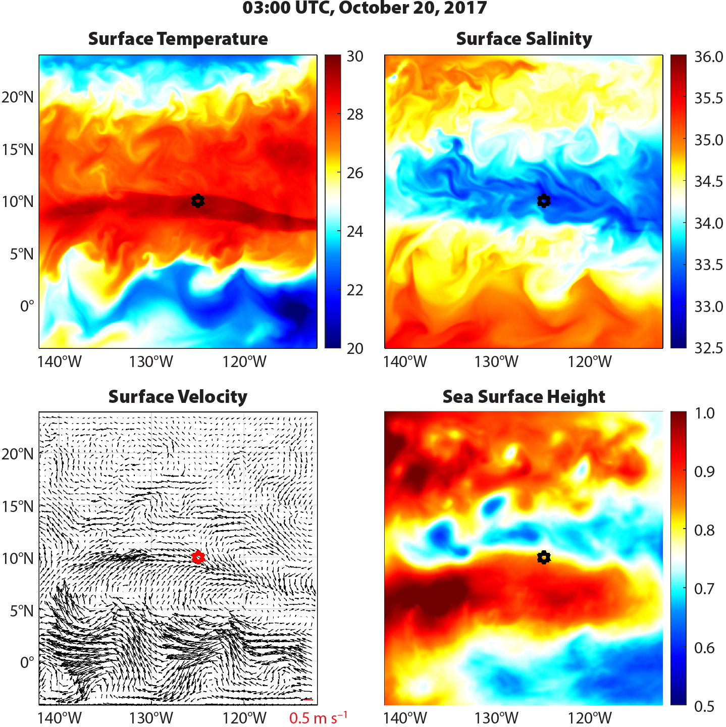
• As the cruises proceeded, brief analysis and forecast reports were prepared to summarize oceanic conditions crucial for SPURS-2. This information was delivered to the SPURS-2 chief scientist and the data management support team on the cruise and to other SPURS-2 investigators through email. As an example, Figure 1 shows the 48-hour forecast that was used in the brief report prepared on October 18, 2017, and valid for October 20.

 

Figure 1. Forty-eight-hour forecast of sea surface temperature, sea surface salinity, surface velocity, and sea surface height valid at 03:00 UTC, October 20, 2017. The forecast is produced using the multiscale data assimilation and forecasting system for SPURS-2. The six-point stars indicate the location of the central mooring. The high salinity filament south of the central mooring is likely real. It is part of an anticyclonic eddy south of the SPURS-2 site. The cyclonic eddy is real as the track of one drifter has shown. > High res figure

 

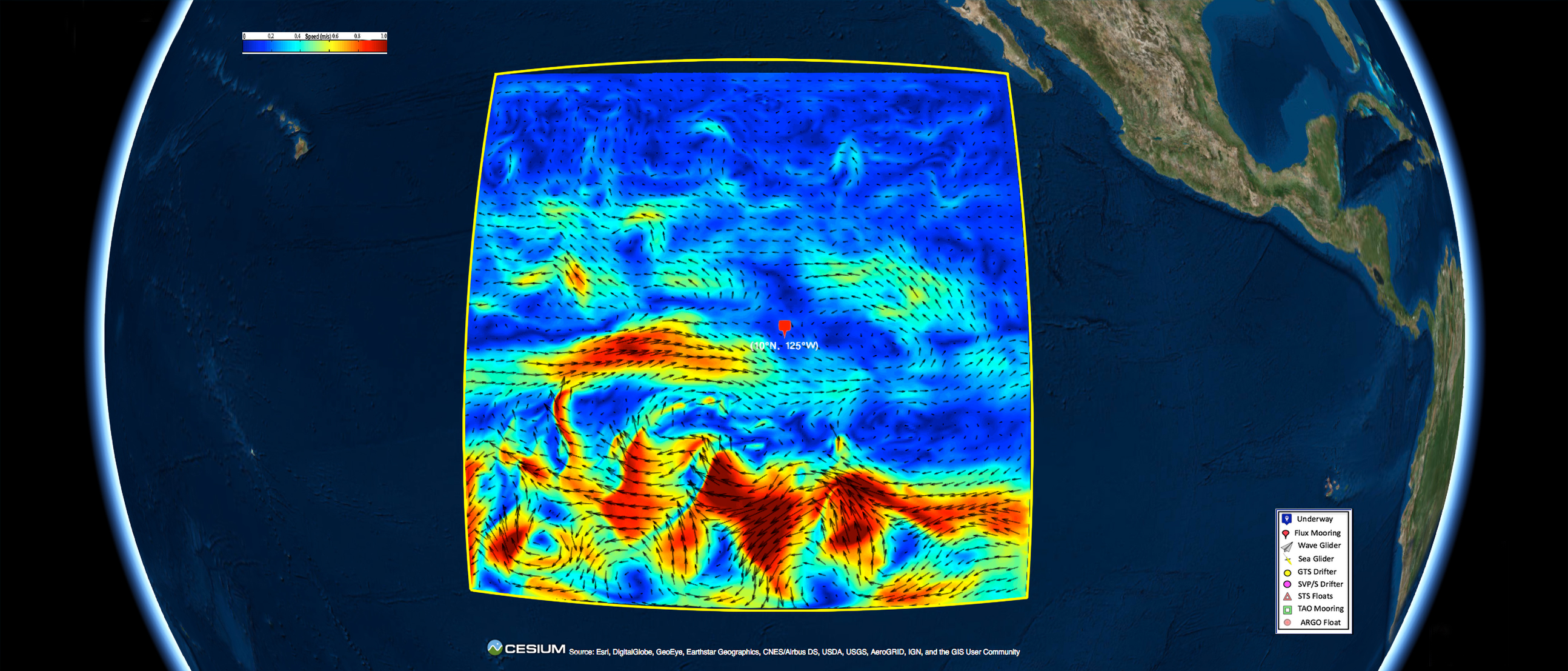
• A subset of the model data assimilation analysis and forecast outputs were posted on the SPURS-2 website (https://ourocean3.jpl.nasa.gov/spurs2/​visual.php). The web page allows users to browse and visualize the analyses and forecasts interactively. The title page image for this article is a screenshot of the visualization page, which displays surface velocity and direction and allows users to zoom in, overlay different data sets, and perform many other analysis tasks, as described by Bingham et al. (2015).
   
• We provided a set of compressed files that included subsets of the model data assimilation analysis and forecast outputs along with atmospheric forecasts and satellite data. This allowed SPURS-2 investigators to gain awareness of current and future oceanic and atmospheric conditions in a size that they could download within the bandwidth constraints of the ship.

After the field experiment, the data assimilation system was used to produce a reanalysis product that quantifies contributions of different processes to the region’s salinity variability. The model output is available to SPURS-2 investigators and the broader community through the SPURS-2 website to enable various diagnostic analyses.

 

Modeling and Data Assimilation

As discussed above, the SPURS-2 field campaign was designed to study physical processes from small to large scales. Thus, we configured the modeling system to represent those scales to a maximum degree. The SPURS-2 model resolves the submesoscale down to a few kilometers because intense vertical velocities associated with submesoscale flows can play an important role in vertical mixing (McWilliams, 2016).

 

Modeling System

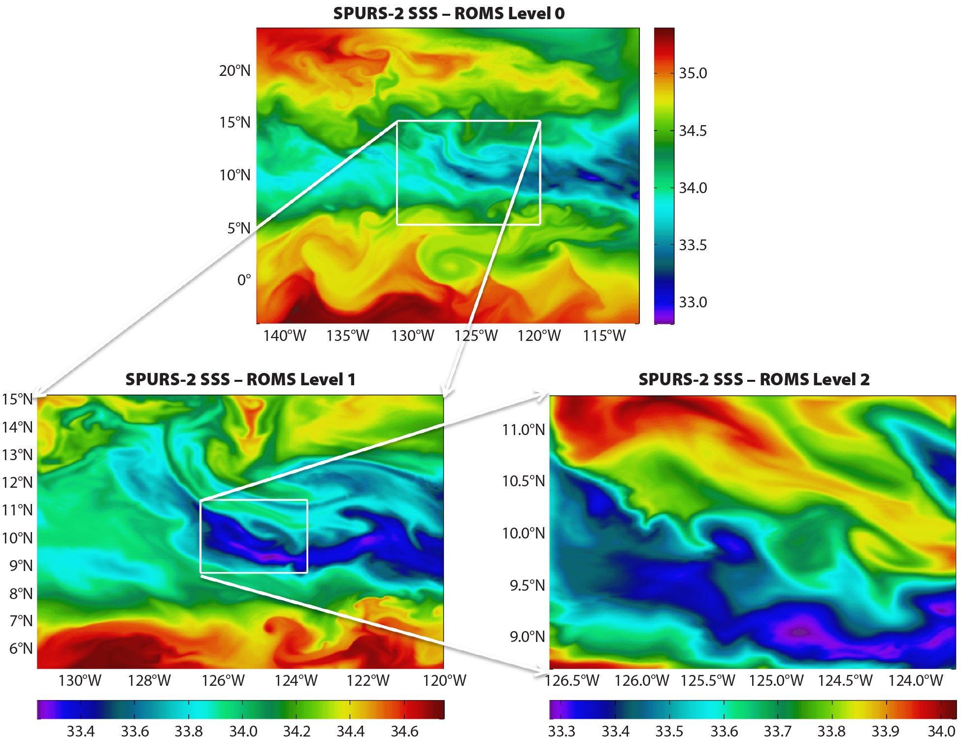
The modeling system was based on the Regional Ocean Modeling System (ROMS; Shchepetkin and McWilliams 2005). ROMS solves the primitive equations in terrain-following coordinates using the full equation of state for seawater (Shchepetkin and McWilliams, 2011). For SPURS-2, ROMS was configured with a set of nested domains as shown in Figure 2. The large-scale ROMS domain covers the tropical and subtropical eastern North Pacific, an area of about 4,000 km × 3,500 km, centered at the SPURS-2 location near (10°N, 125°W). This domain satisfies the requirement to realistically reproduce flow features associated with equatorial upwelling, tropical instability waves (TIWs), and observed high and low salinity bands (Fiedler and Talley, 2006; Guimbard et al., 2017; Melnichenko et al., 2019, in this issue). The model domain has a meridional scale much larger than the width of the fresh SSS band centered around 10°N, with a spatial resolution of 9 km.

 

Figure 2. Three nested model domains at resolutions of 9 km (top), 3 km (bottom left), and 1 km (bottom right) as described in the text. Colors show simulated sea surface salinity (SSS in psu) from the nested domains on October 1, 2015. Note different color scales for each panel. > High res figure

 

Two smaller ROMS domains with increasing spatial resolution, 3 km for the middle domain and 1 km for the small domain, are nested within this large-scale domain. The 3 km and 1 km ROMS domain sizes were selected based on our experience with SPURS-1 and recent studies that show the importance of submesoscale circulations at spatial scales in a range from a few kilometers to tens of kilometers in the region (Su et al., 2018). The goal for these nested domains was to resolve horizontal spatial scales in the range of a 1–2 km to a few hundreds of kilometers, thus encompassing the mesoscale and submesoscale. In the vertical, there are 52 levels, with a grid spacing of about 2 m near surface. These fine resolution models allow us to effectively assimilate the SPURS-2 measurements from ship-based instruments, including underway thermosalinographs, mooring profilers, acoustic Doppler current profilers (ADCPs), XBT/XCTD/UCTD transects, Seagliders, salinity drifters, floats, Wave Gliders, and others.

Rainfall at the SPURS-2 location tends to be associated with isolated convection systems, and thus can be very patchy (Clayson et al., 2019; Rutledge et al., 2019, both in this issue). Patchy and heavy rainfall results in surface puddles with sharp lateral boundaries (Drushka et al., 2019, in this issue). If concentrated within a small patch, baroclinic and barotropic responses to such concentrated fresh­water fluxes would be expected.

To derive the rainfall and other atmospheric forcing, we used analyses and forecasts from the medium-range Global Forecast System (GFS) at NOAA’s National Centers for Environmental Prediction (NCEP). The NCEP GFS has an equivalent horizontal resolution of about 18 km. At this resolution, the forecasts are made out to seven days. Our experience with the US west coast region shows that the atmospheric forcing at this resolution for driving the ROMS model is adequate. However, this resolution was not sufficient to resolve rainfall distributions associated with isolated convection systems. Thus, patchy and heavy rainfall that leads to surface puddles with sharp lateral boundaries is not represented in the ROMS simulation.

 

Data Assimilation

We implemented an MSDA scheme to assimilate not only observations from SPURS-2 but also those from routine and operational observing networks (Li et al., 2015a,b).

 

Observations

During the past two decades, both satellite remote sensing of the marine environment and in situ underwater autonomous vehicle technologies have been advancing at an unprecedented pace. Based on these technologies, a variety of observing networks has been established. Data sets based on these networks are routinely available, often in real or near-real time. We briefly summarize the routinely available observations that are assimilated into the model.

Temperature/salinity vertical profiles are provided by the global Argo float network and the Tropical Atmosphere Ocean (TAO) mooring array. Although the Argo profiles are spatially and temporally sparse, they allow production of a suite of monthly average data sets. We assimilated data from version 4 of the Met Office Hadley Centre ‘‘EN’’ series (Good et al., 2013), which resolves three-​dimensional T/S fields on spatial scales larger than 300 km and thus can be used to constrain the model bias.

There are three to five altimetry satellites in orbit simultaneously. Collectively, the measurements from these satellites are able to resolve SSH spatial scales larger than 150 km in global averages and larger than 250 km in the tropics (e.g., Chelton et al., 2007; Pujol et al., 2016). The altimetry satellites thus constitute a large mesoscale observing network. Daily SSH maps can be generated by merging SSH measurements from all these satellites. Daily maps produced by the AVISO (Archiving, Validation and Interpretation of Satellite Oceanographic data) project (Pujol et al., 2016) were also assimilated into the SPURS-2 ROMS.

Satellite remote sensing has provided accurate global SSTs for many years. SSTs measured by satellite microwave sensors have a spatial resolution of 25 km, and those measured by infrared (IR) sensors have a spatial resolution of about 1 km. SST measurements are available up to a couple of times daily. The IR SSTs allow resolution of features down to the submesoscale.

Currently, two satellites measure SSS using passive microwave sensors that offer relatively low spatial resolution due to the longer wavelength of microwaves. Together, the measurements allow the generation of daily maps at a spatial resolution on the order of 0.5 degrees.

As described above, a web of SPURS-2 sensors provided a wide range of measurements (Bingham et al., 2019, in this issue) in real time. We assimilated all the available T/S measurements and processed them in real time.

 

Data Assimilation Method

Because the model encompasses a wide range of temporal and spatial scales, an MSDA scheme is used to constrain all the various scales using observations at disparate resolutions (Li et al., 2015a,b). Briefly, the model state at a given time can be written as a vector, consisting of three-dimensional values of temperature, salinity, velocity components, and two-dimensional SSH at all model grid points. A standard three-dimensional variational data assimilation (3DVAR) algorithm can then be used to find a solution that minimizes a cost function associated with these variables, and the obtained solution is known as an optimal estimate.

In the standard 3DVAR, the cost function applies to all spatial scales. However, Li et al. (2015a,b) show that 3DVAR has deficiencies when it is applied to a high-resolution model, such as the SPURS-2 model, that encompasses a wide range of spatial scales. Therefore, a multiscale 3DVAR (MS-3DVAR) was formulated to apply 3DVAR to distinct spatial scales, which were then estimated sequentially. MS-3DVAR suppresses scale aliasing, incorporates a scale-dependent dynamic balance, and mitigates the ineffectiveness of 3DVAR in the assimilation of high-resolution observations along with sparse and low-resolution satellite observations. More details can be found in Li et al. (2015b). With this MS-3DVAR, all the observations described in the above Observations section were effectively assimilated simultaneously.

 

Performance of the Real-Time Analysis and Forecasting System

The data assimilation and forecasting system was developed before R/V Roger Revelle initially sailed to the SPURS-2 region on August 12, 2016. Using the system, we produced ocean state analyses and forecasts out to three days on a daily basis from August 12, 2016, until the end of the SPURS-2 campaign on November 30, 2017. The evaluation will focus on a time period of eight months from March 31 through November 30, 2017, and forecasts from 24 to 48 hours.

 

Mesoscale Eddies

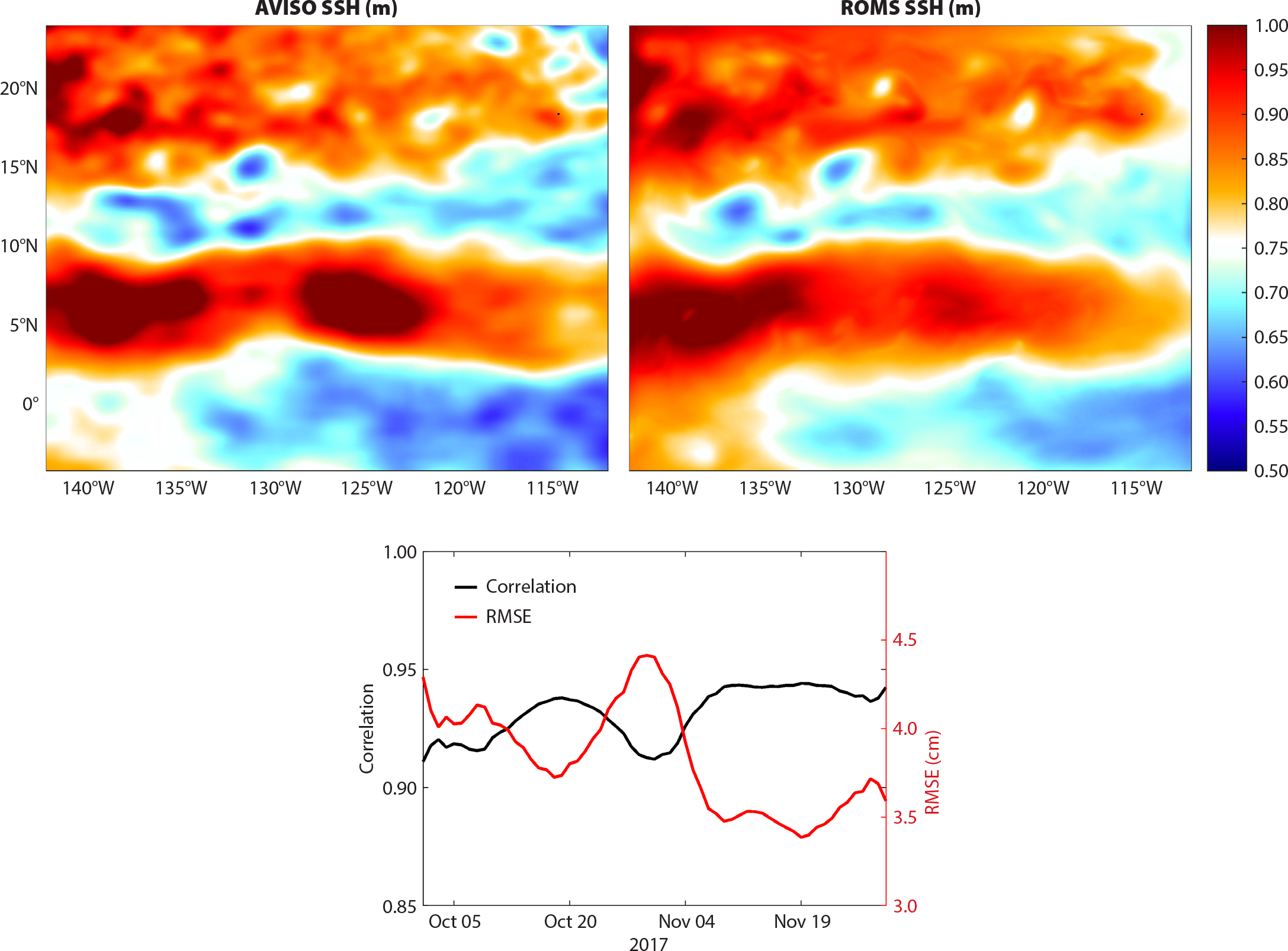
Prediction of mesoscale eddies and other mesoscale features is one of the most important objectives of the SPURS-2 modeling effort. In the sea surface height map shown in Figure 1, energetic eddies with diameters of several hundred kilometers are located near the equator and down to tens of kilometers at the latitude of the SPURS-2 mooring site and further north. The currents associated with these eddies horizontally advect and mix water masses of different salinity. They also impact the trajectories of observing platforms such as drifters and floats, and thus need to be considered when deploying some platforms, particularly the SPURS-2 array of Lagrangian platforms (Lindstrom, et. al., 2017; Shcherbina, et al. 2019, in this issue). Figure 3 gives an example comparison of the daily mean of the model forecast with the AVISO daily SSH. It shows that all the major mesoscale features are comparable between the AVISO data and model forecast SSHs. The spatial correlation between the daily AVISO SSH and the model forecast daily mean SSH is close to or above 0.9 on a daily basis, and the root-mean-square error (RMSE) is smaller than 0.045 m. A correlation of larger than 0.9 indicates that the model forecasts realistically reproduce the location and spatial structure of major mesoscale features. The AVISO SSH resolves eddies down to 250 km in size (Pujol et al., 2016), and thus SSH features of spatial scales smaller than 250 km account for the major part of the RMSE. Because the amplitude of mesoscale eddies in the region is on the order of 0.5 m (Farrar and Weller, 2006), the evaluation indicates that the model forecasts at least accurately reproduce mesoscale eddies that the AVISO SSH can resolve.

 

Figure 3. (top left) AVISO sea surface height (SSH) for October 23, 2017. (top right) Model forecast SSH averaged from 24 to 48 hours, valid on October 23, 2017. (bottom) Spatial correlations and RMSEs of the 24-hour forecast (e.g., top right), evaluated against the AVISO gridded satellite altimetry (e.g., top left). The spatial correlation and RMSE are calculated on a daily basis from October 1 through November 30, 2017, which covers the time period of the second SPURS-2 cruise. > High res figure

 

Velocities Near the Surface

Velocity forecasts were of particular importance to the SPURS-2 field campaign for determining the timing of and locations for the release of the Lagrangian component. However, the forecast of near surface velocities is a continuing challenge to a data assimilation and forecasting system.

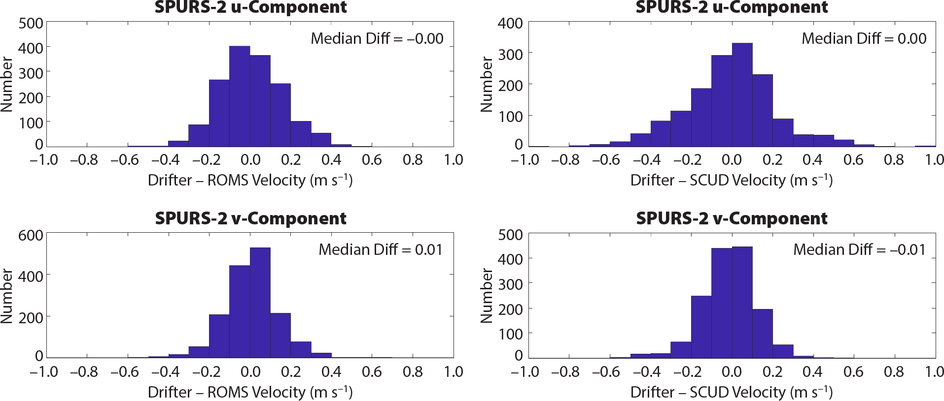
During the campaign, 131 surface drifters drogued at depths of 15 m were used. Among them, 123 were deployed by a group from Scripps Institution of Oceanography (SIO), six were launched by a group from NOAA’s Atlantic Oceanographic and Meteorological Laboratory (AOML) (Lindstrom et al., 2017), and two were drawn from NOAA’s operational drifter network. The drifter data collected between March 31 and November 30, 2017, were used whenever the drifters were located in the 3 km resolution model domain (Figure 2). Velocities were calculated between individual, usually 30-minute, fixes. The daily average of the 3 km 24-hour forecast ROMS velocities at 15 m depth were computed and compared to daily averaged drifter velocities. Model velocities were linearly interpolated in space to the locations of the daily averaged drifter locations to determine matchup values.

Figure 4 shows histograms of the differences between the drifter and the model velocities and gives median differences. The velocity forecast does not indicate any significant bias. The root-mean square of the difference is 0.15 m s^–1 for the zonal component and 0.12 m s^–1 for the meridional component. The average drifter velocity during the period of time is 0.75 m s^–1 for the zonal component and 0.45 m s^–1 for the meridional component, so the error is about 20% to 25%.

 

Figure 4. Histograms of differences between the drifter velocity and the ROMS forecast velocity and between the drifter velocity and the SCUD velocity. The top row shows the zonal (u) component and the bottom row the meridional (v) component. The left column is for ROMS, and the right column for SCUD. Median values of the differences (in m s–1) are given at the top of each panel. > High res figure

 

As a reference, the comparison between the drifter velocities and the SCUD (Surface CUrrents from a Diagnostic model) data product is also given in Figure 4. SCUD is an estimate of upper-ocean velocities computed from a diagnostic model. SCUD uses satellite wind and altimetry, regressed locally with available drifter data, to expand the latter onto a global, ¼-degree daily grid. The values given are best estimates of currents at 15 m (Maximenko and Hafner, 2010). The root mean square of the difference between the SCUD and drifter velocity is 0.22 m s^–1 for both zonal and meridional components. The results presented in Figure 4 indicate that forecast velocities near the surface from a high resolution model with data assimilation can have an accuracy better than those derived purely from observations. As discussed in the Mesoscale Eddies section, the SSH fields related to large-scale eddies from the model forecast are very close to AVISO SSH fields. Because the geostrophic velocities derived from the AVISO SSH are used in the calculation of the SCUD velocity, the velocity fields related to large-scale eddies are close to each other, between those from the ROMS model and the SCUD data. Therefore, the better accuracy of the model velocity results primarily from the small scales that are not resolved by the AVISO SSH but are resolved by the high resolution model.

During the field campaign, we made available real-time comparisons between drifter trajectories, SCUD data, and the model forecast velocities through a visualization page (https://ourocean3.jpl.nasa.gov/spurs2/visual.php). Those comparisons show that the model predicts eddies that the AVISO data cannot resolve.

 

Vertical Profiles

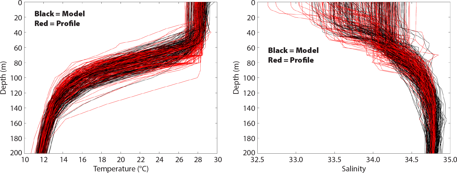
During the field campaign, a portion of observed T/S vertical profiles were not received or processed in real time. Thus, they were not assimilated into the model during the field campaign and are independent data that can be used for model evaluation. Figure 5 shows a comparison between the model forecast and observed T/S vertical profiles that were not assimilated. The observed profiles are from floats deployed by SPURS-2 investigators during the campaign.

 

Figure 5. Comparisons of vertical profiles of temperature (left) and salinity (right). The observations are displayed in red curves and the model forecasts in black curves. The model profiles were taken at the same time and location as the observed ones. > High res figure

 

The model forecast shows high skill in forecasting temperature profiles. The RMSE is less than 0.6°C at all depths. For the salinity profiles, a majority were accurately predicted with a RMSE of less than 0.05 psu. However, there is a group of vertical profiles from the model forecast that shows a significant salty bias near the surface. Those vertical profiles were mostly associated with extremely low values of salinity near the surface, which indicates that low salinity associated with heavy rains were not accurately predicted by the model.

 

Summary and Discussion

Simulation, data assimilation, and numerical forecasting were identified as an integral component of SPURS-2. Thus, we developed an MSDA forecasting system to support the SPURS-2 field campaign. Before the field experiment, the system was used to produce a multiple year simulation and perform OSSEs to aid observing system design. During the field experiment, real-time data assimilation analyses and mesoscale and submesoscale forecasts were provided to SPURS-2 investigators on a daily basis. After the field experiment, models were used to produce a reanalysis product to further address SPURS-2 science questions.

The modeling system produced skillful data assimilation analyses and forecasts. The forecast SSH fields show that the major mesoscale features are comparable with the AVISO data (Figure 3), indicating that the model forecasts at least accurately reproduce mesoscale eddies that the AVISO SSH can resolve. The skillful forecast of currents near the surface (Figure 4) is encouraging. A velocity error of less than 25% renders the current forecasts useful for planning work at sea. The forecast of temperature vertical profiles (Figure 5) is highly accurate. The system accurately forecasts salinity vertical profiles in most of the locations, though extremely low salinity near the surface due to patchy rainfall is still challenging.

We emphasize that the skillful forecasts of mesoscale variability are not derived solely from the SPURS-2 observations, because the SPURS-2 observations took place in a localized area. It is the assimilation of data from routinely available observing networks, particularly satellite altimetry and the Argo network, that primarily constrain mesoscale variability. In fact, these routine observations can only constrain mesoscales down to about 250 km and render the forecast skillful at that scale. This result is of particular importance to the design of future field campaigns. A field campaign should be designed to provide observations that augment the routine observing networks to resolve smaller scales and higher frequency variability, and/or measure variables that the routine observing networks do not provide.

Li, Z., F.M. Bingham, and P.P. Li. 2019. Multiscale simulation, data assimilation, and forecasting in support of the SPURS-2 field campaign. Oceanography 32(2):134–141, https://doi.org/10.5670/oceanog.2019.221.

Bingham, F.M., V. Tsontos, A. deCharon, C.J. Lauter, and L. Taylor. 2019. The SPURS-2 eastern tropical Pacific field campaign data collection. Oceanography 32(2):142–149, https://doi.org/​10.5670/oceanog.2019.222.
1. Bingham, F.M., P. Li, Z. Li, Q. Vu, and Y. Chao. 2015. Data management support for the SPURS Atlantic field campaign. Oceanography 28(1):46–55, https://doi.org/10.5670/oceanog.2015.13.
2. Busecke, J., A.L. Gordon, Z. Li, F.M. Bingham, and J. Font. 2014. Subtropical surface layer salinity budget and the role of mesoscale turbulence. Journal of Geophysical Research 119:4,124–4,140, https://doi.org/10.1002/2013JC009715.
3. Chelton, D.B., M. Schlax, R. Samelson, and R. DeSzoeke. 2007. Global observations of large ocean eddies. Geophysical Research Letters 34, https://doi.org/10.1029/2007GL030812.
4. Clayson, C.A., J.B. Edson, A. Paget, R. Graham, and B. Greenwood. 2019. The effects of rainfall on the atmosphere and the ocean during SPURS-2. Oceanography 32(2):86–97, https://doi.org/​10.5670/oceanog.2019.216.
5. Drushka, K., W.E. Asher, A.T. Jessup, E. Thompson, S. Iyer, and O. Clark. 2019. Capturing fresh layers with the surface salinity profiler. Oceanography 32(2):76–85, https://doi.org/​10.5670/oceanog.2019.215.
6. Farrar, J.T., and A.J. Plueddemann. 2019. On the factors driving upper-ocean salinity variability at the western edge of the Eastern Pacific Fresh Pool. Oceanography 32(2):30–39, https://doi.org/​10.5670/oceanog.2019.209.
7. Farrar, J.T., and R.A. Weller. 2006. Intraseasonal variability near 10°N in the eastern tropical Pacific Ocean. Journal of Geophysical Research 111, C05015, https://doi.org/10.1029/2005JC002989.
8. Fiedler, P.C., and L.D. Talley. 2006. Hydrography of the eastern tropical Pacific: A review. Progress in Oceanography 69:143–180, https://doi.org/10.1016/​j.pocean.2006.03.008.
9. Good, S.A., M.J. Martin, and N.A. Rayner. 2013. EN4: Quality controlled ocean temperature and salinity profiles and monthly objective analyses with uncertainty estimates. Journal of Geophysical Research 118:6,704-6,716, https://doi.org/​10.1002/​2013JC009067.
10. Guimbard, S., N. Reul, B. Chapron, M. Umbert, and C. Maes. 2017. Seasonal and interannual variability of the Eastern Tropical Pacific Fresh Pool. Journal of Geophysical Research 122:1,749– 1,771, https://doi.org/​10.1002/​2016JC012130.
11. Li, Z., J.C. McWilliams, K. Ide, and J.D. Fararra. 2015a. A multi-scale data assimilation scheme: Formulation and illustration. Monthly Weather Review 143:3,804–3,822, https://doi.org/10.1175/MWR-D-14-00384.1.
12. Li, Z., J.C. McWilliams, K. Ide, and J.D. Fararra. 2015b. Coastal ocean data assimilation using a multi-scale three-dimensional variational scheme. Ocean Dynamics 65:1,001–1,015, https://doi.org/​10.1007/s10236-015-0850-x.
13. Lindstrom, E., F. Bryan, and R. Schmitt. 2015. SPURS: Salinity Processes in the Upper-ocean Regional Study—The North Atlantic Experiment. Oceanography 28(1):14–19, https://doi.org/10.5670/oceanog.2015.01.
14. Lindstrom, E.J., A.Y. Shcherbina, L. Rainville, J.T. Farrar, L.R. Centurioni, S. Dong, E.A. D’Asaro, C. Eriksen, D.M. Fratantoni, B.A. Hodges, and others. 2017. Autonomous multi-platform observations during the Salinity Processes in the Upper-ocean Regional Study. Oceanography 30(2):38–48, https://doi.org/​10.5670/oceanog.2017.218.
15. Maximenko, N., and J. Hafner. 2010. SCUD: Surface CUrrents from Diagnostic model. IPRC Technical Note No. 5, February 16, 2010, 17 pp.
16. McWilliams, J.C. 2016. Submesoscale currents in the ocean. Proceedings of the Royal Society A 472:20160117, https://doi.org/10.1098/rspa.2016.0117.
17. Melnichenko, O., P. Hacker, F.M. Bingham, and T. Lee. 2019. Patterns of SSS variability in the eastern tropical Pacific: Intraseasonal to interannual time scales from seven years of NASA satellite data. Oceanography 32(2):20–29, https://doi.org/​10.5670/oceanog.2019.208.
18. Pujol, M.-I., Y. Fauguere, G. Taburet, S. Dupuy, C. Pelloquin, M. Ablain, and N. Picot. 2016. DUACS DT2014: The new multi-mission altimeter data set reprocessed over 20 years. Ocean Science 12:1,067–1,090, https://doi.org/10.5194/os-12-1067-2016.
19. Rainville, L., L.R. Centurioni, W.E. Asher, C.A. Clayson, K. Drushka, J.B. Edson, B.A. Hodges, V. Hormann, J.T. Farrar, J.J. Schanze, and A.Y. Shcherbina. 2019. Novel and flexible approach to access the open ocean: Uses of sailing research vessel Lady Amber during SPURS-2. Oceanography 32(2):116–121, https://doi.org/10.5670/oceanog.2019.219.
20. Rutledge, S.A, V. Chandrasekar, B. Fuchs, J. George, F. Junyent, P. Kennedy, and B. Dolan. 2019. Deployment of the SEA-POL C-band polarimetric radar to SPURS-2. Oceanography 32(2):50–57, https://doi.org/10.5670/oceanog.2019.212.
21. SPURS-2 Planning Group. 2015. From salty to fresh—Salinity Processes in the Upper-ocean Regional Study-2 (SPURS-2): Diagnosing the physics of a rainfall-dominated salinity minimum. Oceanography 28(1):150–159, https://doi.org/​10.5670/oceanog.2015.15.
22. Shchepetkin, A.F., and J.C. McWilliams. 2005. The Regional Oceanic Modeling System (ROMS): A split-explicit, free-surface, topography-​following-​coordinate oceanic model. Ocean Modelling 9:347–404, https://doi.org/10.1016/​j.ocemod.2004.08.002.
23. Shchepetkin, A.F., and J.C. McWilliams. 2011. Accurate Boussinesq oceanic modeling with a practical, stiffened equation of state. Ocean Modelling 38:41–70, https://doi.org/10.1016/j.ocemod.2011.01.010.
24. Shcherbina, A.Y., E.A. D’Asaro, and R.R. Harcourt. 2019. Rain and sun create slippery layers in the Eastern Pacific Fresh Pool. Oceanography 32(2):98–107, https://doi.org/​10.5670/oceanog.2019.217.
25. Su, Z., J. Wang, P. Klein, A.F. Thompson, and D. Menemenlis. 2018. Ocean submesoscales as a key component of the global heat budget. Nature Communications 9, 775, https://doi.org/10.1038/s41467-018-02983-w.

This is an open access article made available under the terms of the Creative Commons Attribution 4.0 International License (https://creativecommons.org/licenses/by/4.0/), which permits use, sharing, adaptation, distribution, and reproduction in any medium or format as long as users cite the materials appropriately, provide a link to the Creative Commons license, and indicate the changes that were made to the original content. Images, animations, videos, or other third-party material used in articles are included in the Creative Commons license unless indicated otherwise in a credit line to the material. If the material is not included in the article’s Creative Commons license, users will need to obtain permission directly from the license holder to reproduce the material.