Ocean forecast models rely on observations to provide regular updates in order to correctly represent dynamic ocean circulation. This synthesis of observations and models is referred to as data assimilation. Since initial conditions dominate the quality of short-term ocean forecasts, accurate ocean state estimates, achieved through data assimilation, are key to improving prediction. Western boundary current (WBC) regions are particularly challenging to model and predict because they are highly variable. Understanding how specific observation types, platforms, locations, and observing frequencies impact model estimates is key to effective observing system design.

The East Australian Current (EAC), the South Pacific’s WBC, is a relatively well-observed current system that allows us to study the impact of observations on prediction across different dynamical regimes, from where the current flows as a mostly coherent jet to the downstream eddy field. Here we present a review of the impact of observations on model estimates of the EAC using three different methods. Consistent results across the three approaches provide a comprehensive understanding of observation impact in this dynamic WBC. Observations made in regions of greater natural variability contribute most to constraining the model estimates, and subsurface observations have a high impact relative to the number of observations. Significantly, sampling the downstream eddy-rich region constrains the upstream circulation, whereas observing the upstream coherent jet provides less improvement to downstream eddy field estimates. Studies such as these provide powerful insights into both observing system design and modeling approaches that are vital for optimizing observation and prediction efforts.

Introduction

Accurate estimates of past, present, and future ocean states are crucial to effective management of our ocean environment and marine industries. Short-term ocean predictions (days to weeks) are vital to myriad environmental, societal, and economic applications, including facilitating the adaptive management of marine ecosystems, forecasting extreme weather events, predicting the onset and persistence of marine heatwaves, providing accurate ocean forecasts for shipping and military operations, predicting the fate of pollutants, and guiding search and rescue operations.

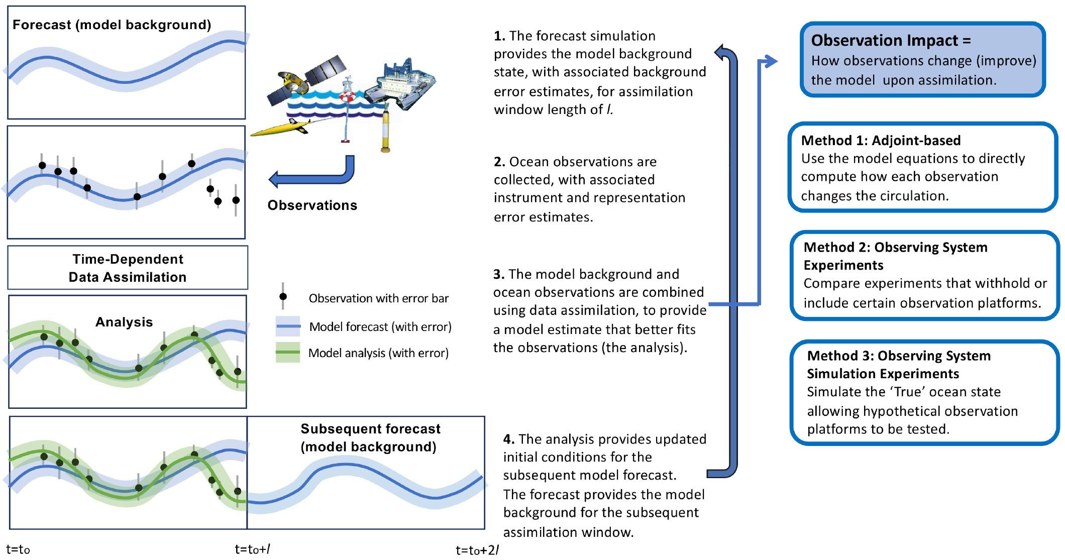
Ocean state estimates require the combination of numerical models and ocean observations, referred to as data assimilation (DA). Observations provide sparse data points while the model provides dynamical context. The goal of DA is to combine the model with observations to reduce uncertainty in the model estimate. For forecasting purposes, model estimates are updated through assimilation when observations become available and provide improved initial conditions for the next forecast (Figure 1). Due to the dynamic nature of the ocean circulation, ocean models must be regularly updated through DA to, for example, correctly represent the timing and locations of oceanic eddies (e.g., Thoppil et al., 2021; Chamberlain et al., 2021).

 

FIGURE 1. Conceptual schematic showing sequential time-dependent data assimilation and a summary of the three methods presented in this study for assessing observation impact. > High res figure

 

A critical component of the DA problem is the way by which the information contained in the observations is projected onto the (unobserved) model state estimate. Advanced DA techniques use time-variable model dynamics to actively interpolate information from observations up- and downstream and forward and backward in time. Observations are assimilated over a time interval, given the temporal evolution of the circulation (e.g., Moore et al., 2020). Identifying observations that best constrain an ocean model can drive improved observing system design for more accurate and more cost-effective prediction. Observation impact studies aim to quantify how specific observation types, locations, and observing frequencies impact model estimates (e.g., Oke et al., 2015).

In this article, we assess observation impact in a dynamic western boundary current (WBC). WBCs are swift, poleward-flowing currents that exist on the western sides of subtropical ocean gyres. They transport warm water from the tropics toward the poles, redistributing heat and modulating global climate. Mesoscale eddies form due to instabilities in the strong boundary current flow, making WBC extension regions hotspots of high eddy variability (Imawaki et al., 2013; Li et al., 2022a). WBCs typically exhibit the highest errors in ocean forecasts (e.g., Brassington et al., 2023) due to their strong flows, the complexities of eddy shedding and evolution (e.g., Kang and Curchitser, 2013; Pilo et al., 2015; Yang et al., 2018), and their complex vertical structures (e.g., Sun et al., 2017; Pilo et al., 2018; Brokaw et al., 2020; Rykova and Oke, 2022). Understanding the interplay of observing system design and modeling approaches is crucial to improving prediction in highly dynamic, eddy-rich oceanographic environments.

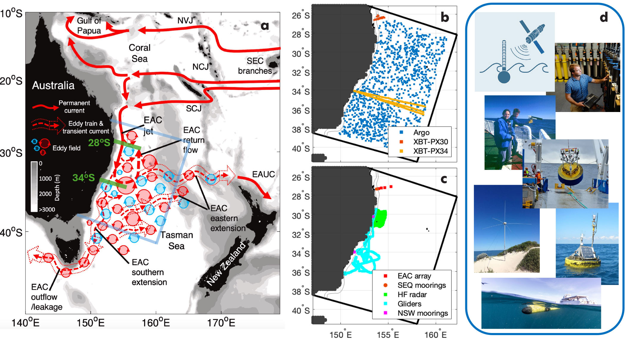
The East Australian Current (EAC) is the WBC of the South Pacific subtropical gyre, and its eddies dominate the circulation along the southeastern coast of Australia (Figure 2a; Oke et al., 2019). The southward-flowing current is most coherent off 28°S (Sloyan et al., 2016) and intensifies around 29°–31°S (Kerry and Roughan, 2020). The current typically separates from the coast between 31°S and 32.5°S, turning eastward and shedding large warm-core eddies in the Tasman Sea (Cetina Heredia et al., 2014). The EAC is a relatively well-observed WBC system, with observations collected as part of Australia’s Integrated Marine Observing System (IMOS; Figure 2b–d) spanning from the coherent jet to the eddy field (e.g., Roughan et al., 2015). The EAC therefore provides an ideal testbed for assessing observation impact across differing dynamical regimes.

 

FIGURE 2. The EAC is a fairly well observed western boundary current system. (a) Schematic showing the East Australia Current (EAC; adapted from Oke et al., 2019) with the regional ocean model domain. (b) Locations of Argo and eXpendable BathyThermograph (XBT) observations. (c) Integrated Marine Observing System (IMOS) observations. (d) Photos of observing the EAC. Photo credits: M. Roughan and IMOS. > High res figure

 

Observing networks, numerical models, and DA schemes make up the key components of ocean prediction systems. Data-assimilating models are useful for evaluating and designing observing networks. Here we synthesize the results from three different model-based approaches in order to assess observation impact across a common system (the EAC). We use three methods for studying observation impact: an adjoint-based approach to directly quantify observation impact, Observing System Experiments (withholding observations), and Observing System Simulation Experiments (Figure 1). This review summarizes the key results obtained through each method, and synthesizes the consistent results to provide a broad understanding of observation impact along the extent of the WBC system.

 

Assessing Observation Impact

The South East Australian Coastal Forecast System

The South East Australian Coastal Forecast System (SEA-COFS) consists of several Regional Ocean Modeling System (ROMS; Shchepetkin and McWilliams, 2005) configurations at a range of resolutions for the southeast Australian oceanic region. The EAC-ROMS regional model (domain shown in Figure 2a) has a 2.5–5 km horizontal resolution, with higher resolution over the continental shelf and slope, and 30 terrain-following vertical layers (Kerry et al., 2016; Kerry and Roughan, 2020).

We constrain the model with observational data from a variety of traditional and novel observation platforms using four-dimensional variational DA (4D-Var). This technique uses variational calculus to solve for increments in model initial conditions, boundary conditions, and forcing such that the differences between the new model solution of the time-evolving flow and all available observations is minimized—in a least-squares sense—over an assimilation window (Figure 1; Moore et al., 2004, 2011). Here we use five-day assimilation windows. The goal is for the model to represent all of the observations in time and space using the physics of the model, and accounting for the uncertainties in the observations and background model state, to produce a description of the ocean state that is a dynamically consistent solution of the nonlinear model equations. For this mesoscale eddy-dominated system, adjustments to the initial conditions dominate over boundary or surface forcing adjustments and forecast errors are dominated by errors in the initial state (Kerry et al., 2020).

Observation impact is studied based on a data-​assimilating configuration of the EAC-ROMS model for 2012–2013 (Kerry et al., 2016), when numerous data streams were available through IMOS (Figure 2b,c). These included velocity and hydrographic observations from a deep-​water mooring array (the EAC array; Sloyan et al., 2016) and continental shelf moorings (Malan et al., 2021; Roughan et al., 2022), radial surface velocities from a high-​frequency (HF) radar array (Archer et al., 2017), and hydrographic observations from ocean gliders (Schaeffer et al., 2016). These observations complemented the more traditional data streams of satellite-derived sea surface height (SSH) and sea surface temperature (SST), temperature and salinity from Argo profiling floats, and temperature from eXpendable BathyThermograph (XBT) lines.

Method 1: An Adjoint-Based Approach

The 4D-Var DA scheme uses sequential iterations of the linearized model equations and their adjoint (Errico, 1997) to minimize the model-observation difference. By defining a scalar measure of the ocean circulation, we can use this mathematical framework to directly compute the impact of each individual observation on the change in the circulation measure (e.g., Langland and Baker, 2004; Powell, 2017). We use this methodology to understand how observations impact estimates of alongshore volume transport through shore-normal sections that span the extent of the EAC, and of spatially averaged eddy kinetic energy (EKE) over the eddy-rich Tasman Sea (Kerry et al., 2018).

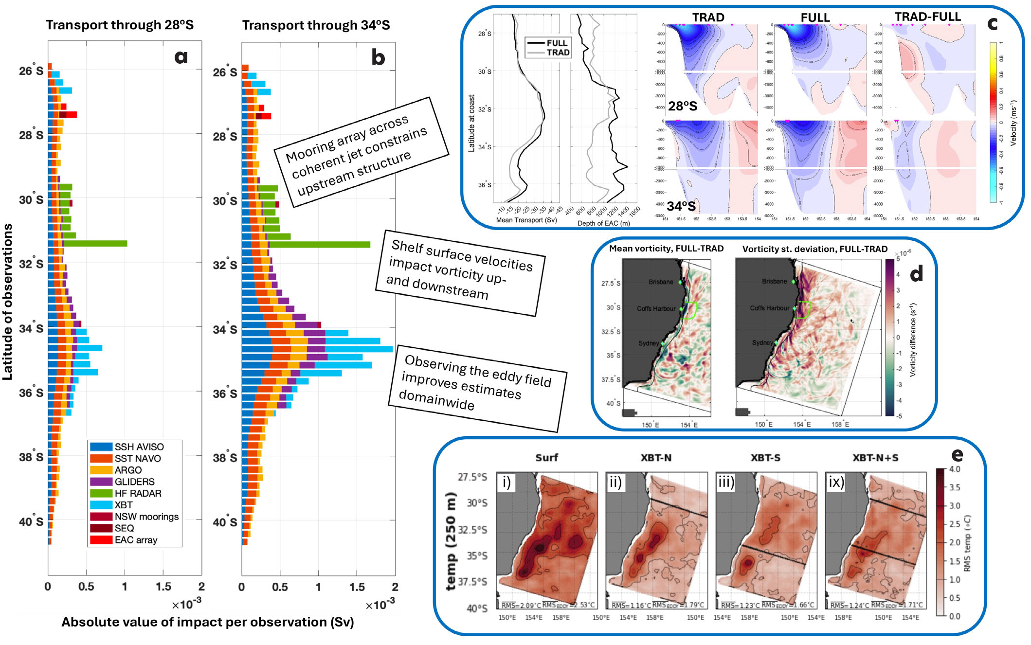
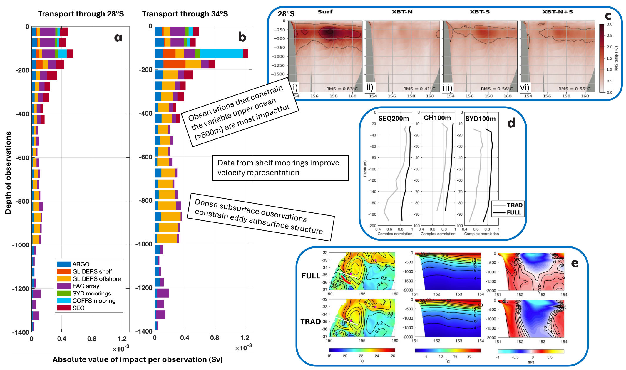
The contribution of each observing platform to changes in modeled volume transport and EKE varies considerably over the two-year period, as it depends on the flow regime and the observation coverage for each assimilation window. To gain an overall picture of how observations from across the EAC region impact a particular circulation metric, we group the observation impacts by acquisition latitude (Figure 3a,b). This analysis reveals that both up- and downstream observations impact transport estimates along the extent of the EAC system. While the EAC is mostly coherent off 28°S, volume transport varies due to meandering of the EAC core and intermittent separation events (Oke et al., 2019; Kerry and Roughan, 2020). Glider and XBT observations off 34°S and HF radar observations at 30°S impact EAC transport to the north (28°S, upstream impacts, Figure 3a). The volume transport off 34°S is more variable than upstream due to the eddy-dominated circulation regime (Kerry and Roughan, 2020). This downstream transport is constrained primarily by observations over the eddy field but is also impacted by the EAC array, the northern XBT lines, and the HF radar observations (downstream impacts, Figure 3b).

 

FIGURE 3. Summary of up- and downstream observation impacts. (a) Observation impacts using the adjoint-based method on transport through the shore normal section crossing the coast at 28°S (upstream) grouped into latitude bins of 0.25° and normalized by the number of observations. (b) Same as (a) but for transport through section crossing the coast at 34°S (downstream). Adapted from Kerry et al. (2018) (c) Observing System Experiments (OSEs) show the EAC mooring array constraining upstream current structure (Siripatana et al., 2020). (d) Surface radial velocities (from HF radar array at 30°S) impact vorticity up- and downstream (Siripatana et al., 2020). (e) Observing System Simulation Experiments (OSSEs) show that subsurface temperature (250 m) is improved with XBT observations (Gwyther et al., 2022). Text in the black boxes summarizes parallels between the information in panels a–b and that in panels c–e. AVISO = Archiving, Validation, and Interpretation of Satellite Oceanographic data. EAC = East Australia Current. HF = High frequency. SEQ = South East Queensland. SSH = Sea surface height. SST = Sea surface temperature. NAVO = Naval Oceanographic Office. NSW = New South Wales. XBT = eXpendable BathyThermograph. See text for definitions of FULL and TRAD. > High res figure

 

Normalizing the impacts by the number of observations (e.g., Figure 3a,b) reveals that observations over the eddy field make the greatest contribution to volume transport estimates along the coast. SSH, SST, and Argo observations made in the region of high eddy variability (33°–37°S) have more impact than the same observations made elsewhere as they provide information to constrain the variable region. Even for volume transport estimates where the jet is mostly coherent, satellite and Argo observations of the (downstream) eddy field have greater impact than the same observation types upstream (Figure 3a). The eddy field observation impact exceeds the impact of observations local to 28°S.

Subsurface observations that sample hydrography within EAC eddies, such as those from Argo, gliders, and XBTs, are also particularly impactful (Figure 3a,b). Observations made in the upper 500 m of the water column contribute more to changes in the circulation estimates than deeper observations (Figure 4a,b). When glider observations sample eddies offshore of the continental shelf (Figure 2c), they have large impacts on EAC transport and EKE (contributing to 28%–36% of transport increments, and 38% for EKE; Kerry et al., 2018).

 

FIGURE 4. Summary of subsurface observation impacts. (a) Observation impacts using the adjoint-based method on transport through the shore normal section crossing the coast at 28°S (upstream) grouped into depth bins and normalized by the number of observations. (b) Same as (a) but for transport through section crossing the coast at 34°S (downstream). Adapted from Kerry et al. (2018) (c) OSSEs show the depth region of greatest variability (>500 m) benefits most from subsurface observations (Gwyther et al., 2022). (d) OSEs show improvement in shelf velocities with mooring data assimilated (Siripatana et al., 2020). (e) Example of glider data (glider path shown in red) constraining the subsurface temperature and velocity structure of a cold core eddy off Sydney (Siripatana et al., 2020). Text in the black boxes summarizes parallels between the information in panels a–b and that in panels c–e. SEQ = Southeast Queensland. CH and COFFS = Coffs Harbor. SYD = Sydney. > High res figure

 

Method 2: Observing System Experiments

Observing System Experiments (OSEs) compare the results of a DA system that withholds certain observations with a system that includes them (e.g., Chang et al., 2023). Using the EAC-ROMS configuration for 2012–2013, we compared the impact of assimilating only the more traditional observations (satellite-derived SSH and SST, and vertical profiles from Argo and XBTs: the TRAD experiment), versus also including data from more novel observation platforms (HF radar, deep and shallow moorings, and gliders: the full suite of all available observations, the FULL experiment; Siripatana et al., 2020).

While the overall surface and subsurface properties were well represented with assimilation of surface observations and sparse subsurface profiles (TRAD), including mooring, radar, and glider observations (FULL) further improved ocean state estimates. Specifically, shelf mooring observations improved temperature and velocity estimates inshore of the EAC (e.g., Figure 4d), and HF radar observations covering the continental shelf and slope at 30°S were key to representing vorticity (Siripatana et al., 2020). The inclusion of HF radar data resulted in increased cyclonic vorticity inshore of the EAC both up- and downstream of the HF radar location and increased vorticity variance (Figure 3d). This increase in cyclonic vorticity is confirmed as an improvement under the HF radar footprint (by comparison to the assimilated surface radial velocity observations). Without independent observations, we cannot confirm that this increased vorticity is an improvement in the up- and downstream regions, but it is reasonable to assume that the velocity shear structure inshore of the EAC extends up- and downstream of 30°S and that FULL provides improved representation of this.

Despite the shelf and slope circulation being improved in the FULL analyses, at the end of five-day forecasts, the predictive skill over the shelf was equivalent to that of the TRAD forecasts (Kerry et al., 2024b). For these same experiments, Kerry et al. (2020) show that downscaling to a finer resolution (1 km) coastal/shelf model was more effective at maintaining the vorticity gradient in the five-day forecasts, although correctly predicting the timing and location of fine-scale features, specifically cyclonic eddies that form inshore of the EAC, remains a challenge.

The width of the EAC core and the mean EAC transport with latitude was well constrained across both experiments (TRAD and FULL). Assimilation of observations from the EAC mooring array constrained the core depth over the 27°–30°S region (FULL), while the core extended too deep in their absence (TRAD). However, poleward of 30°S, the average depth of the EAC core extended too deep in the FULL compared to the TRAD experiment (Figure 3c; Siripatana et al., 2020). Glider observations of hydrographic structure were effective in constraining eddy depth when they sampled offshore eddies. When they were available (an approximately three-month period in 2013), eddies constrained by glider data (FULL) showed realistic eddy depths compared to the TRAD case where the eddy depths extended well below the typical level of no motion (e.g., Figure 4e).

Method 3: Observing System Simulation Experiments

Assessment of ocean prediction systems is limited as a large portion of the ocean state is unobserved, particularly below the surface. Observing System Simulation Experiments (OSSEs) are designed to replicate a realistic prediction system; by defining a given model solution as the Truth (or Nature run), the system can then be evaluated everywhere against a known ocean state (e.g., Gasparin et al., 2019; Kerry and Powell, 2022). Synthetic observations are extracted from the Truth and assimilated into a Baseline model (or Twin), which represents the background numerical model (refer to Kerry et al., 2024a; Figure 1). Errors are intentionally introduced into the Baseline model (e.g., in initial conditions and boundary and surface forcing) to mimic the uncertainties in a realistic prediction system. Often a Nature run is sought with a higher resolution and some degree of independence (e.g., different model physics) from the Baseline model (e.g., Halliwell et al., 2017).

In the EAC-ROMS configuration, a series of OSSEs were performed to assess the impact of alternate locations and frequencies of subsurface temperature observations (Gwyther et al., 2022, 2023a, 2023b). These experiments compare the impact of assimilating (synthetic) surface-​​only observations that mimic satellite derived SSH and SST (SURF) with experiments that also include (synthetic) repeat XBT lines (subsurface temperature profiles) through the upstream EAC region (XBT-N), the downstream region (XBT-S), and both the up- and downstream regions (XBT-N+S; Figure 3e).

The OSSEs show that subsurface temperature observations are key to improved representation of the EAC system below the surface. Observing the downstream, eddy-​dominated region has a strong impact on improving EAC subsurface structure both up- and downstream of the observing location (Gwyther et al., 2022, 2023a). Observing the mostly coherent upstream region (XBT-N) gave the best fit across that section but was less effective in improving subsurface estimates in the downstream region, while observing across the downstream section (XBT-S) gave comparatively lower errors across the domain (Figure 3e). Including both observation platforms (XBT-N+S) gave the lowest errors across the domain, but the gain in skill was small relative to XBT-S alone (Figure 3e). A sampling frequency close to the assimilation window length (weekly XBT lines in this case) resulted in considerable improvement in subsurface representation across the eddy field compared to fortnightly and greater periods between samples (Gwyther et al., 2023b).

 

Synergies Across the Three Methods

Here, we apply three different methods (Figure 1), each with unique advantages and limitations, to assess observation impact in the EAC. The adjoint-based method (Method 1) allows us to quantify the contribution of each individual observation to the change in a given target metric between the forecast and the analysis. This then allows us to pinpoint exactly which data (from a large set of assimilated constraints) are most valuable in the assimilation system. The impacts relate to changes in the specifically defined circulation metrics, but the degree of improvement is unknown as the true ocean state is not known away from observed locations. The relative impacts of the different observation platforms are specific to the chosen circulation measure. OSEs (Method 2) compare model skill for experiments that withhold or include different platforms, but interpretation is limited as, again, the true state is unknown. OSSEs (Method 3) address this shortcoming by simulating a complete representation of the “true” ocean state. Drawbacks associated with OSSE design include correctly representing background model error so that the system represents a realistic system. By employing all three methods across a common system we can comprehensively assess observation impact across the EAC region. The synergy between the results provides confidence in the overarching findings.

Up- and Downstream Impacts

Time-dependent DA methods, like 4D-Var, account for the time-evolving flow so localized observation platforms can have far-reaching impacts. Respecting the model dynamics, information captured by the observations propagates in time and space and influences the unobserved ocean state. For example, changes to surface velocities at a certain time and location (an example of an observed variable) must be balanced by changes to surface and isopycnal tilt, with adjustments both up- and downstream and forward and backward in time.

Surface velocity observations from an HF radar array at 30°S impact EAC volume transport both up- and downstream as well as downstream EKE (Figure 3a,b). OSEs revealed the influence of these observations on vorticity along the extent of the EAC and the vorticity variance (Figure 3d). More generally, observations taken over the latitudinal extent of the EAC system were shown to influence transport estimates both up- and downstream (Figure 3a,b). Measuring the upstream coherent jet impacts downstream transport estimates, and observing the eddies downstream constrains upstream estimates. The propagation of information from the downstream to the upstream is found to be more effective in improving model skill away from the observed location (see the section below).

Observing the (Downstream) Eddy Field

The adjoint-based method revealed that observations of the eddy field have higher impacts on transport estimates along the EAC than the same observations taken in the less variable regions. Surface observations of the eddy field impacted upstream transport more than surface observations over the coherent jet (Figure 3a). OSEs showed that while mooring observations across the jet resulted in improved skill in the upstream (27°–30°S) region, EAC transport and subsurface structure in the downstream region were not improved (Figure 3c). The value of observing the downstream region was confirmed by the OSSEs, which show the advantage of subsurface observations through the eddy field compared to observations through the coherent jet (Figure 3e). While the strength of the upstream jet can be a predictor of separation latitude in general (Li et al., 2022b), it provides little skill in predicting the downstream evolution of the current instabilities and resultant eddies. In contrast, observing the location where instabilities are growing into eddies gives information on both the conditions that fed the instability (upstream) and how the eddy will further evolve (downstream).

Observing Below the Surface

The value of subsurface observations is revealed across all three observation impact methodologies. EAC transport and eddies (geostrophic flow) should be constrained by both surface observations (that inform surface tilt) and subsurface observations (that inform isopycnal tilt). Given the dynamical context provided by the model, the surface tilt associated with mesoscale eddies should be projected below the surface to alter the isopycnal tilt. However, in practice, the impact of surface observations in constraining the subsurface is limited (e.g., Zavala-Garay et al., 2012). While the adjoint-based method quantifies the relative impact of the surface observations on circulation changes, the OSEs and OSSEs reveal that the depth structure of the EAC is degraded upon assimilation of surface observations alone (Siripatana et al., 2020; Gwyther et al., 2022, 2023a, 2023b; Figure 4c(i)). The adjoint-based method shows that in situ observations in the upper 500 m contribute most to changes in EAC transport and EKE (compared to deeper observations, Figure 4a,b) as they provide information on the structure of the mixed layer and the pycnocline. Glider observations within eddies informed transport estimates some 900 km upstream and 300 km downstream. The OSSEs showed that repeated subsurface temperature observations across the eddy-dominated region improved subsurface temperature estimates over the entire EAC region (Figure 3e). The depth region of greatest variability (>500 m) showed the highest errors upon assimilation of surface only observations and benefited most from subsurface observations (Figure 4c).

 

Feedback Between Models and Observations

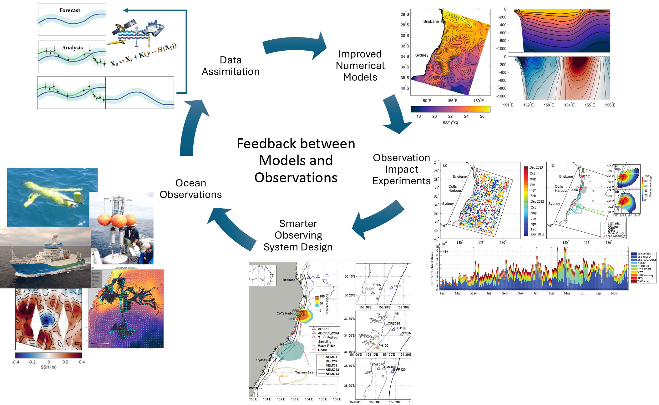
Observing networks for ocean prediction must be designed with specific goals, and a continuous feedback loop should exist between numerical models and observations (Figure 5). Ocean models, observing systems, and DA schemes must evolve and adapt together for optimal benefit. Observation impact studies are a crucial part of this feedback loop as they can quantify the value of specific observations, identify regions where data gaps are most detrimental to model estimates, and drive improvements in modeling and DA systems.

 

FIGURE 5. Conceptual schematic of the feedback loop between models and observations for continuously evolving ocean prediction systems. > High res figure

 

Observation impact experiments have shown the specific value of various novel observing platforms, motivating their sustained implementation. For example, surface velocity observations from localized HF radar platforms have shown widespread improvement in surface current representation in eddy-rich regions (Siripatana et al., 2020; Kerry et al., 2020; Couvelard et al., 2021). Dense subsurface hydrographic observations (from gliders or profiles) in eddies drove improvements in EAC eddy field and upstream representation (Kerry et al., 2018; Siripatana et al., 2020; Gwyther et al., 2022, 2023a, 2023b). The challenges of piloting gliders in regions of strong and variable currents limit the sustained availability of such observations, and novel opportunistic methods of obtaining subsurface data, such as fishing vessel observation networks (Jakoboski et al., 2024), are emerging.

The value of observing different dynamical regions was shown in the EAC, where observing the downstream instabilities was more useful than observing the upstream jet. This provides valuable information for observing system design in oceanic regions where eddies form from current instabilities, such as WBC regions (e.g., Kang and Curchitser, 2015; Yang et al., 2018) and the North Pacific’s subtropical countercurrent (Qiu, 1999). The value of in situ observations of the variable upper ocean was highlighted (Kerry et al., 2018), consistent with findings in other regions (e.g., Powell, 2017; Geng et al., 2020; Kerry et al., 2022). Furthermore, we show that different circulation regimes may require different sampling strategies (Gwyther et al., 2022), motivating adaptive sampling (e.g., Mourre and Alvarez, 2012; Gao et al., 2022).

The value of observations is limited by the spatial and temporal resolution of the model (e.g., Oke and Sakov, 2008), the processes resolved (e.g., Kerry and Powell, 2022), the DA scheme (e.g., Kerry et al., 2024b), observational errors, and redundancy with other elements of the observing system (e.g., Loose and Heimbach, 2021). Observation impact experiments can not only drive smarter observing system design but also model and DA system improvements. For example, studying the assimilation increments and assessing predictive skill over the continental shelf adjacent to the EAC showed that shelf processes were not adequately resolved in a regional model (Kerry et al., 2020, 2024b). This result revealed that higher resolution models are required to resolve and forecast shelf flows. In a region of strong internal tides and mesoscale eddies, observation impact experiments showed the value of resolving both tides and eddies in the background numerical model for improved prediction of both processes (Kerry and Powell, 2022).

The DA system should be configured to draw optimum benefit from the observations. DA is particularly challenging in regions of complex circulation, such as eddy-rich regions and shelf seas, which are typically under-sampled and where the circulation contains a broad range of temporal and spatial scales. Advanced time-dependent assimilation schemes, such as 4D-Var and the Ensemble Kalman Filter, are crucial for capturing highly intermittent flows with irregularly sampled observations (e.g., Raynaud et al., 2011; Moore et al., 2020; Kerry et al., 2024b). Observation impact studies have shown the importance of the DA system configuration in handling dense, localized observations (e.g., Pasmans et al., 2019; Kerry et al., 2024a). Optimizing DA schemes requires ongoing development, and future advances should include the development of hybrid methods, nested and coupled DA, and the ability to ingest new and emerging observing platforms (Moore et al., 2019; Pasmans et al., 2020).

 

Conclusions

Numerical models, observing networks, and data assimilation techniques are the key interconnected components of an ocean prediction system. There is a need for robust and consistent model-based design and evaluation of observing networks that are scale and region appropriate. Such frameworks can inform fit-for-purpose observing strategies, identify gaps in observation systems, and drive improvements in model and data assimilation methodologies. Data-assimilating ocean models need to be evaluated against independent observations and below the surface. Assessment of models against assimilated surface and sparse profile data gives little insight into model performance away from the observed locations.

Here, we present a complementary set of methods that can provide powerful insights into model-based design and evaluation of observing networks. Each method exhibits unique advantages and limitations. By employing all three methods across a common system, we provide a holistic assessment of observation impacts. The results are specific to the numerical model’s configuration and resolution, the circulation regime, the distinct observing networks, and the data assimilation system; however, key messages provide parallels to other regions and other systems. Our methods focus on improved ocean state estimates, since initial conditions dominate the quality of short-term ocean forecasts. It is noted that atmospheric forcing errors might be important for longer forecast horizons.

While these and similar methods have been used to guide observing system design in other regions globally, this study is the first of its kind to use three distinct methods to converge toward recommendations. Key outstanding challenges include representing complex subsurface oceanic structures with sparse observations, dealing with localized dense observations, and assimilating data in regions where the circulation varies over a broad range of temporal and spatial scales. Our results point to the importance of feedback between numerical modeling, ocean observing systems, and data assimilation methodology in driving improved estimates of the ocean environment.

 

Competing Interests

No competing interests are present.

 

Acknowledgments

This research was supported by Australian Research Council grants DP140102337, LP160100162, and LP170100498 to MR. Synthesis of the results was supported by LP220100515 to SK. MR and CK acknowledge funding from the Australian Research Council for the South East Australian Coastal Ocean Forecast System (SEA-COFS), including grants DP230100505, LP220100515, LP170100498, LP160100162, LP150100064, DP140102337, and LP1201005922023. The authors would also like to thank the two anonymous reviewers, whose suggestions improved this manuscript.

Kerry, C., M. Roughan, S. Keating, and D. Gwyther. 2025. Model-based observing system evaluation in a western boundary current: Observation impact from the coherent jet to the eddy field. In Frontiers in Ocean Observing. E.S. Kappel, V. Cullen, I.C.A. da Silveira, G. Coward, C. Edwards, P. Heimbach, T. Morris, H. Pillar, M. Roughan, and J. Wilkin, eds, Oceanography 38(Supplement 1), https://doi.org/10.5670/oceanog.2025e110.

1. Archer, M., M. Roughan, S. Keating, and A. Schaeffer. 2017. On the variability of the East Australian Current: Jet structure, meandering, and influence on shelf circulation. Journal of Geophysical Research: Oceans 122(11):8,464–8,481, https://doi.org/10.1002/2017JC013097.
2. Brassington, G.B., P. Sakov, P. Divakaran, A. Aijaz, J. Sweeney-Van Kinderen, X. Huang, and S. Allen. 2023. OceanMAPS v4.0i: A global eddy resolving EnKF ocean forecasting system. In OCEANS 2023 – Limerick. Conference held June 5–8, 2023, Limerick, Ireland, IEEE, https://doi.org/10.1109/OCEANSLimerick52467.2023.10244383.
3. Brokaw, R.J., B. Subrahmanyam, C.B. Trott, and A. Chaigneau. 2020. Eddy surface characteristics and vertical structure in the Gulf of Mexico from satellite observations and model simulations. Journal of Geophysical Research: Oceans 125:e2019JC015 538, https://doi.org/​10.1029/2019JC015538.
4. Cetina Heredia, P., M. Roughan, E. Van Sebille, and M. Coleman. 2014. Long-term trends in the East Australian Current separation latitude and eddy driven transport. Journal of Geophysical Research: Oceans 119(7):4,351–4,366, https://doi.org/10.1002/2014JC010071.
5. Chamberlain, M., P. Oke, G. Brassington, P. Sandery, P. Divakaran, and R. Fiedler. 2021. Multiscale data assimilation in the Bluelink ocean reanalysis (BRAN). Ocean Modelling 166:101849, https://doi.org/​10.1016/j.ocemod.2021.101849.
6. Chang, I., Y.H. Kim, H. Jin, Y.-G. Park, G. Pak, and Y.-S. Chang. 2023. Impact of satellite and regional in-situ profile data assimilation on a high-resolution ocean prediction system in the Northwest Pacific. Frontiers in Marine Science 10:1085542, https://doi.org/10.3389/fmars.2023.1085542.
7. Couvelard, X., C. Messager, P. Penven, S. Smet, and P. Lattes. 2021. Benefits of radar-derived surface current assimilation for South of Africa ocean circulation. Geoscience Letters 8(5), https://doi.org/10.1186/s40562-021-00174-y.
8. Errico, R.M. 1997. What is an adjoint model? Bulletin of the American Meteorological Society 78:2,577–2,592, https://doi.org/​10.1175/​1520-​0477(1997)078<2577:WIAAM>2.0.CO;2.
9. Gao, Z., G. Chen, Y. Song, J. Zheng, and C. Ma. 2022. Adaptive network design for multiple gliders observation of mesoscale eddy. Frontiers in Marine Science 9:823397, https://doi.org/10.3389/fmars.2022.823397.
10. Gasparin, F., S. Guinehut, C. Mao, I. Mirouze, E. Rémy, R.R. King, M. Hamon, R. Reid, A. Storto, P.-Y. Le Traon, and others. 2019. Requirements for an integrated in situ Atlantic Ocean observing system from coordinated observing system simulation experiments. Frontiers in Marine Science 6:83, https://doi.org/10.3389/fmars.2019.00083.
11. Geng, W., F. Cheng, Q. Xie, X. Zou, W. He, Z. Wang, Y. Shu, G. Chen, D. Liu, D. Ye, and others. 2020. Observation system simulation experiments using an ensemble-based method in the northeastern South China Sea. Journal of Oceanology and Limnology 38:1,729–1,745, https://doi.org/​10.1007/s00343-019-9119-4.
12. Gwyther, D.E., C. Kerry, M. Roughan, and S.R. Keating. 2022. Observing system simulation experiments reveal that subsurface temperature observations improve estimates of circulation and heat content in a dynamic western boundary current. Geoscientific Model Development 15:6,541–6,565, https://doi.org/10.5194/gmd-​15-​6541-2022.
13. Gwyther, D.E., S.R. Keating, C. Kerry, and M. Roughan. 2023a. How does 4DVar data assimilation affect the vertical representation of mesoscale eddies? A case study with observing system simulation experiments (OSSEs) using ROMS v3.9. Geoscientific Model Development 162023:157–178, https://doi.org/10.5194/gmd-16-157-2023.
14. Gwyther, D.E., M. Roughan, C. Kerry, and S.R. Keating. 2023b. Impact of assimilating repeated subsurface temperature transects on state estimates of a western boundary current. Frontiers in Marine Science 9:1084784, https://doi.org/10.3389/fmars.2022.1084784.
15. Halliwell, G.R. Jr., M.F. Mehari, M. Le Hénaff, V.H. Kourafalou, I.S. Androulidakis, H.S. Kang, and R. Atlas. 2017. North Atlantic Ocean OSSE system: Evaluation of operational ocean observing system components and supplemental seasonal observations for potentially improving tropical cyclone prediction in coupled systems. Journal of Operational Oceanography 10:154–175, https://doi.org/10.1080/1755876X.2017.1322770.
16. Imawaki, S., A. Bower, L. Beal, and B. Qiu. 2013. Western boundary currents. Pp. 305–338 in Ocean Circulation and Climate: A 21^st Century Perspective. G. Siedler, S.M. Griffies, J. Gould, and J.A. Church, eds, Elsevier, https://doi.org/10.1016/B978-0-12-391851-2.00013-1.
17. Jakoboski, J., M. Roughan, J. Radford, J.M.A.C. de Souza, M. Felsing, R. Smith, N. Puketapu-Waite, M.M. Orozco, K.H. Maxwell, and C. Van Vranken. 2024. Partnering with the commercial fishing sector and Aotearoa New Zealand’s ocean community to develop a nationwide subsurface temperature monitoring program. Progress in Oceanography 225:103278, https://doi.org/10.1016/​j.pocean.2024.103278.
18. Kang, D., and E.N. Curchitser. 2013. Gulf Stream eddy characteristics in a high-resolution ocean model. Journal of Geophysical Research: Oceans 118:4,474–4,487, https://doi.org/10.1002/jgrc.20318.
19. Kang, D., and E.N. Curchitser. 2015. Energetics of eddy–mean flow interactions in the Gulf Stream region. Journal of Physical Oceanography 45:1,103–1,120, https://doi.org/10.1175/jpo-d-14-0200.1.
20. Kerry, C.G., B.S. Powell, M. Roughan, and P.R. Oke. 2016. Development and evaluation of a high-resolution reanalysis of the East Australian Current region using the Regional Ocean Modelling System (ROMS 3.4) and Incremental Strong-Constraint 4-Dimensional Variational (IS4D-Var) data assimilation. Geoscientific Model Development 9:3,779–3,801, https://doi.org/10.5194/gmd-9-3779-2016.
21. Kerry, C.G., M. Roughan, and B.S. Powell. 2018. Observation impact in a regional reanalysis of the East Australian Current system. Journal of Geophysical Research: Oceans 123(10):7,511–7,528, https://doi.org/​10.1029/2017JC013685.
22. Kerry, C., and M. Roughan. 2020. Downstream evolution of the East Australian Current system: Mean flow, seasonal, and intra-annual variability. Journal of Geophysical Research: Oceans 125:e2019JC015227, https://doi.org/10.1029/2019JC015227.
23. Kerry, C., M. Roughan, and B. Powell. 2020. Predicting the submesoscale circulation inshore of the East Australian Current. Journal of Marine Systems 204:103286, https://doi.org/10.1016/j.jmarsys.2019.103286.
24. Kerry, C.G., and B.S. Powell. 2022. Including tides improves subtidal prediction in a region of strong surface and internal tides and energetic mesoscale circulation. Journal of Geophysical Research: Oceans 127:e2021JC018314, https://doi.org/10.1029/2021JC018314.
25. Kerry, C., M. Roughan, and J.M. Azevedo Correia de Souza. 2022. Drivers of upper ocean heat content extremes around New Zealand revealed by Adjoint Sensitivity Analysis. Frontiers in Climate 4:980990, https://doi.org/​10.3389/​fclim.2022.980990.
26. Kerry, C., M. Roughan, and J.M. Azevedo Correia de Souza. 2024a. Assessing the impact of subsurface temperature observations from fishing vessels on temperature and heat content estimates in shelf seas: A New Zealand case study using Observing System Simulation Experiments. Frontiers in Marine Science 11:1358193, https://doi.org/​10.3389/fmars.2024.1358193.
27. Kerry, C.G., M. Roughan, S. Keating, D. Gwyther, G. Brassington, A. Siripatana, and J.M.A.C. Souza, 2024b. Comparison of 4-dimensional variational and ensemble optimal interpolation data assimilation systems using a Regional Ocean Modeling System (v3.4) configuration of the eddy-dominated East Australian Current system. Geoscientific Model Development 17:2,359–2,386, https://doi.org/10.5194/egusphere-​2023-2355.
28. Langland, R.H., and N.L. Baker. 2004. Estimation of observation impact using the NRL atmospheric variational data assimilation adjoint system. Tellus A: Dynamic Meteorology and Oceanography 56(3):189–201, https://doi.org/10.3402/tellusa.v56i3.14413.
29. Li, J., M. Roughan, and C. Kerry. 2022a. Drivers of ocean warming in the western boundary currents of the Southern Hemisphere. Nature Climate Change 12:901–909, https://doi.org/10.1038/s41558-022-01473-8.
30. Li, J., M. Roughan, and C. Kerry. 2022b. Variability and drivers of ocean temperature extremes in a warming western boundary current. Journal of Climate 35:1,097–1,111, https://doi.org/10.1175/JCLI-D-21-0622.1.
31. Loose, N., and P. Heimbach. 2021. Leveraging uncertainty quantification to design ocean climate observing systems. Journal of Advances in Modeling Earth Systems 13:e2020MS002386, https://doi.org/​10.1029/2020MS002386.
32. Malan, N., M. Roughan, and C. Kerry. 2021. The rate of coastal temperature rise adjacent to a warming western boundary current is nonuniform with latitude. Geophysical Research Letters 48:e2020GL090751, https://doi.org/10.1029/2020GL090751.
33. Moore, A.M., H.G. Arango, E. Di Lorenzo, B.D. Cornuelle, A.J. Miller, and D.J. Neilson. 2004. A comprehensive ocean prediction and analysis system based on the tangent linear and adjoint of a regional ocean model. Ocean Modelling 7:227–258, https://doi.org/10.1016/​j.ocemod.2003.11.001.
34. Moore, A.M., H.G. Arango, G. Broquet, B.S. Powell, A.T. Weaver, and J. Zavala-Garay. 2011. The Regional Ocean Modelling System (ROMS) 4-dimensional variational data assimilation systems: Part 1. System overview and formulation. Progress in Oceanography 91:34–49, https://doi.org/​10.1016/j.pocean.2011.05.004.
35. Moore, A., M. Martin, S. Akella, H. Arango, M. Balmaseda, L. Bertino, S. Ciavatta, B. Cornuelle, J. Cummings, S. Frolov, and others. 2019. Synthesis of ocean observations using data assimilation for operational, real-time and reanalysis systems: A more complete picture of the state of the ocean. Frontiers in Marine Science 6:90, https://doi.org/​10.3389/fmars.2019.00090.
36. Moore, A., J. Zavala-Garay, H.G. Arango, C.A. Edwards, J. Anderson, and T. Hoar. 2020. Regional and basin scale applications of ensemble adjustment Kalman filter and 4D-Var ocean data assimilation systems. Progress in Oceanography 189:102450, https://doi.org/10.1016/​j.pocean.2020.102450.
37. Mourre, B., and A. Alvarez. 2012. Benefit assessment of glider adaptive sampling in the Ligurian Sea. Deep Sea Research Part I 68:68–78, https://doi.org/10.1016/j.dsr.2012.05.010.
38. Oke, P.R., and P. Sakov. 2008. Representation error of oceanic observations for data assimilation. Journal of Atmospheric and Oceanic Technology 25:1,004–1,017, https://doi.org/10.1175/2007JTECHO558.1.
39. Oke, P.R., G. Larnicol, E.M. Jones, V. Kourafalou, A. Sperrevik, F. Carse, C.A. Tanajura, B. Mourre, M. Tonani, G. Brassington, and others. 2015. Assessing the impact of observations on ocean forecasts and reanalyses: Part 2. Regional applications. Journal of Operational Oceanography 8:s63–s79, https://doi.org/10.1080/1755876X.​2015.1022080.
40. Oke, P.R., M. Roughan, P. Cetina-Heredia, G.S. Pilo, K.R. Ridgway, T. Rykova, M.R. Archer, R.C. Coleman, C.G. Kerry, C. Rocha, and others. 2019. Revisiting the circulation of the East Australian Current: Its path, separation, and eddy field. Progress in Oceanography 176:102139, https://doi.org/​10.1016/j.pocean.2019.102139.
41. Pasmans, I., A.L. Kurapov, J.A. Barth, A. Ignatov, P.M. Kosro, and R.K. Shearman. 2019. Why gliders appreciate good company: Glider assimilation in the Oregon-Washington coastal ocean 4DVAR system with and without surface observations. Journal of Geophysical Research: Oceans 124:750–772, https://doi.org/10.1029/2018JC014230.
42. Pasmans, I., A.L. Kurapov, J.A. Barth, P.M. Kosro, and R.K. Shearman. 2020. Ensemble 4DVAR (En4DVar) data assimilation in a coastal ocean circulation model: Part II. Implementation offshore Oregon–Washington, USA. Ocean Modelling 154:101681, https://doi.org/10.1016/j.ocemod.​2020.101681.
43. Pilo, G.S., M.M. Mata, and J.L.L. Azevedo. 2015. Eddy surface properties and propagation at Southern Hemisphere western boundary current systems. Ocean Science 11:629–641, https://doi.org/10.5194/os-11-629-2015.
44. Pilo, G.S., P.R. Oke, R. Coleman, T. Rykova, and K. Ridgway. 2018. Patterns of vertical velocity induced by eddy distortion in an ocean model. Journal of Geophysical Research: Oceans 123:2,274–2,292, https://doi.org/​10.1002/​2017JC013298.
45. Powell, B.S. 2017. Quantifying how observations inform a numerical reanalysis of Hawaii. Journal of Geophysical Research: Oceans 122(11):8,427–8,444, https://doi.org/10.1002/2017JC012854.
46. Qiu, B. 1999. Seasonal eddy field modulation of the North Pacific Subtropical Countercurrent: TOPEX/Poseidon observations and theory. Journal of Physical Oceanography 29(10):2,471–2,486, https://doi.org/​10.1175/​1520-0485(1999)029<2471:SEFMOT>2.0.CO;2.
47. Raynaud, L., L. Berre, and G. Desroziers. 2011. An extended specification of flow-dependent background error variances in the Météo-France global 4D-Var system. Quarterly Journal of the Royal Meteorological Society 137:607–619, https://doi.org/10.1002/qj.795.
48. Roughan, M., A. Schaeffer, and I.M. Suthers. 2015. Sustained ocean observing along the coast of southeastern Australia: NSW-IMOS 2007–2014. Pp. 76–98 in Coastal Ocean Observing Systems. Y. Liu, H. Kerkering, and R.H. Weisberg, eds, Elsevier.
49. Roughan, M., M. Hemming, A. Schaeffer, T. Austin, H. Beggs, M. Chen, M. Feng, G. Galibert, C. Holden, D. Hughes, and others. 2022. Multi-decadal ocean temperature time-series and climatologies from Australia’s long-term National Reference Stations. Scientific Data 9:157, https://doi.org/10.1038/s41597hy-022-01224-6.
50. Rykova, T., and P.R. Oke. 2022. Stacking of EAC eddies observed from Argo. Journal of Geophysical Research: Oceans 127:e2022JC018 679, https://doi.org/10.1029/2022JC018679.
51. Schaeffer, A., M. Roughan, T. Austin, J.D. Everett, D. Griffin, B. Hollings, E. King, A. Mantovanelli, S. Milburn, B. Pasquer, and others. 2016. Mean hydrography on the continental shelf from 26 repeat glider deployments along southeastern Australia. Scientific Data 3:160070, https://doi.org/10.1038/sdata.2016.70.
52. Shchepetkin, A.F., and J.C. McWilliams. 2005. The regional oceanic modeling system (ROMS): A split-explicit, free-surface, topography-​following-​coordinate oceanic model. Ocean Modelling 9:347–404, https://doi.org/​10.1016/j.ocemod.2004.08.002.
53. Siripatana, A., C. Kerry, M. Roughan, J.M.A. Souza, and S. Keating. 2020. Assessing the impact of nontraditional ocean observations for prediction of the East Australian Current. Journal of Geophysical Research: Oceans 125:e2020JC016580, https://doi.org/10.1029/2020JC016580.
54. Sloyan, B.M., K.R. Ridgway, and R. Cowley. 2016. The East Australian Current and property transport at 27°S from 2012 to 2013. Journal of Physical Oceanography 46(3):993–1,008, https://doi.org/10.1175/JPO-D-15-0052.1.
55. Sun, W., C. Dong, R. Wang, Y. Liu, and K. Yu. 2017. Vertical structure anomalies of oceanic eddies in the Kuroshio Extension region. Journal of Geophysical Research: Oceans 122:1,476–1,496, https://doi.org/​10.1002/​2016JC012226.
56. Thoppil, P.G., S. Frolov, C.D. Rowley, C.A. Reynolds, G.A. Jacobs, E.J. Metzger, P.J. Hogan, N. Barton, A.J. Wallcraft, O.M. Smedstad, and others. 2021. Ensemble forecasting greatly expands the prediction horizon for ocean mesoscale variability. Communications Earth & Environment 2:89, https://doi.org/10.1038/s43247-021-00151-5.
57. Yang, H., B. Qiu, P. Chang, L. Wu, S. Wang, Z. Chen, and Y. Yang. 2018. Decadal variability of eddy characteristics and energetics in the Kuroshio Extension: Unstable versus stable states. Journal of Geophysical Research: Oceans 123:6,653–6,669, https://doi.org/​10.1029/2018JC014081.
58. Zavala-Garay, J., J.L. Wilkin, and H.G. Arango. 2012. Predictability of mesoscale variability in the East Australian Current given strong-constraint data assimilation. Journal of Physical Oceanography 42:1,402–1,420, https://doi.org/10.1175/JPO-D-11-0168.1.

This is an open access article made available under the terms of the Creative Commons Attribution 4.0 International License (https://creativecommons.org/licenses/by/4.0/), which permits use, sharing, adaptation, distribution, and reproduction in any medium or format as long as users cite the materials appropriately, provide a link to the Creative Commons license, and indicate the changes that were made to the original content. Images, animations, videos, or other third-party material used in articles are included in the Creative Commons license unless indicated otherwise in a credit line to the material. If the material is not included in the article’s Creative Commons license, users will need to obtain permission directly from the license holder to reproduce the material.