Mesoscale eddies are important to many aspects of the dynamics of the Arctic Ocean. Among others, they maintain the halocline and interact with the Atlantic Water circumpolar boundary current through lateral eddy fluxes and shelf-basin exchanges. Mesoscale eddies are also important for transporting biological material and for modifying sea ice distribution. Here, we review what is known about eddies and their impacts in the Arctic Ocean in the context of rapid climate change. Eddy kinetic energy (EKE) is a proxy for mesoscale variability in the ocean due to eddies. We present the first quantification of EKE from moored observations across the entire Arctic Ocean and compare those results to output from an eddy resolving numerical model. We show that EKE is largest in the northern Nordic Seas/Fram Strait and it is also elevated along the shelf break of the Arctic Circumpolar Boundary Current, especially in the Beaufort Sea. In the central basins, EKE is 100–1,000 times lower. Generally, EKE is stronger when sea ice concentration is low versus times of dense ice cover. As sea ice declines, we anticipate that areas in the Arctic Ocean where conditions typical of the North Atlantic and North Pacific prevail will increase. We conclude that the future Arctic Ocean will feature more energetic mesoscale variability.

An oceanographic mooring is recovered aboard R/V Polarstern in 2018. Photo credit: W.-J. von Appen. > High res figure

Introduction: Eddies in the Arctic Ocean

During the second half of the twentieth century, physical oceanographers increasingly appreciated that the world ocean is populated by eddies (Warren and Wunsch, 1981) and that they are fundamental to setting ocean stratification and to understanding the dynamics of the global circulation (e.g., Gnanadesikan, 1999). These swirling water motions are the main form of mesoscale variability. The timescales over which these features evolve typically range from a few days to a few months. As the name suggests, the mesoscale ranges from small-scale local effects of tides, individual storms, and mixing on the fast end to large-scale basin-wide circulation on the slow end of the spectrum.

It is more difficult to study eddies in the Arctic Ocean than in lower latitudes, and research addressing them in the Arctic increased significantly only in the past two decades after four major challenges were overcome. First, sea ice cover and harsh weather make the Arctic particularly inaccessible for in situ observations. Second, while lower latitude eddies are observed to have typical horizontal scales of hundreds of kilometers, high latitudes are associated with very small Rossby radii (the typical horizontal scale of eddies) on the order of 1–15 km (Nurser and Bacon, 2014), requiring observations and numerical models to have very high horizontal resolution. Third, satellite remote-sensing products, which have been instrumental for mesoscale research at lower latitudes for decades, are of less value in the Arctic. For instance, sea ice disturbs typical satellite measurements at the sea surface, the prevailing near-freezing temperatures make eddy detection based on sea surface temperature impractical, and the small Rossby radius necessitates high horizontal resolution. In addition, many polar-orbiting satellites have inclinations <75° thereby missing the majority of the Arctic Ocean, although the recent CryoSat mission has improved on this limitation. Fourth, many Arctic eddies exist as subsurface lenses that are obscured from surface observations (e.g., Porter et al., 2020).

Here, we review examples from which insights have been gained on the character and ubiquity of Arctic eddies. These studies are based on ship-based surveys, bottom-moored and ice-based observations, and regional and/or process numerical models designed to overcome the challenges specific to the Arctic Ocean. The eddies are similar in size to the Rossby radius and are the dominant form of mesoscale variability. However, we note that distinguishing eddies from inertial oscillations and tidal variability remains a challenge as the frequencies in question can be very close (Lenn et al., 2021).

The high-resolution (1 km) numerical model of Wang et al. (2020) resolves most eddies. A snapshot of speed from the model (Figure 1a) shows that strong velocities (>0.3 m s^–1) are present in parts of the Arctic Ocean. For example, in Fram Strait it shows small (~30 km diameter) energetic vortices that are formed via baroclinic instability where Atlantic Water recirculates and subducts below Polar Water (Hattermann et al., 2016). These prominent and well-delineated eddies (Johannessen et al., 1987; Figure 2a) are characterized by relatively strong motions of up to 0.5 m s^–1 (Figure 1b,c; von Appen et al., 2016). We consider this an illustrative example of energetic circulation at the boundaries and contrast it with the dynamically much quieter interior basins, such as the Nansen Basin, with water speeds of <0.05 m s^–1 (Figure 1b,c).

 

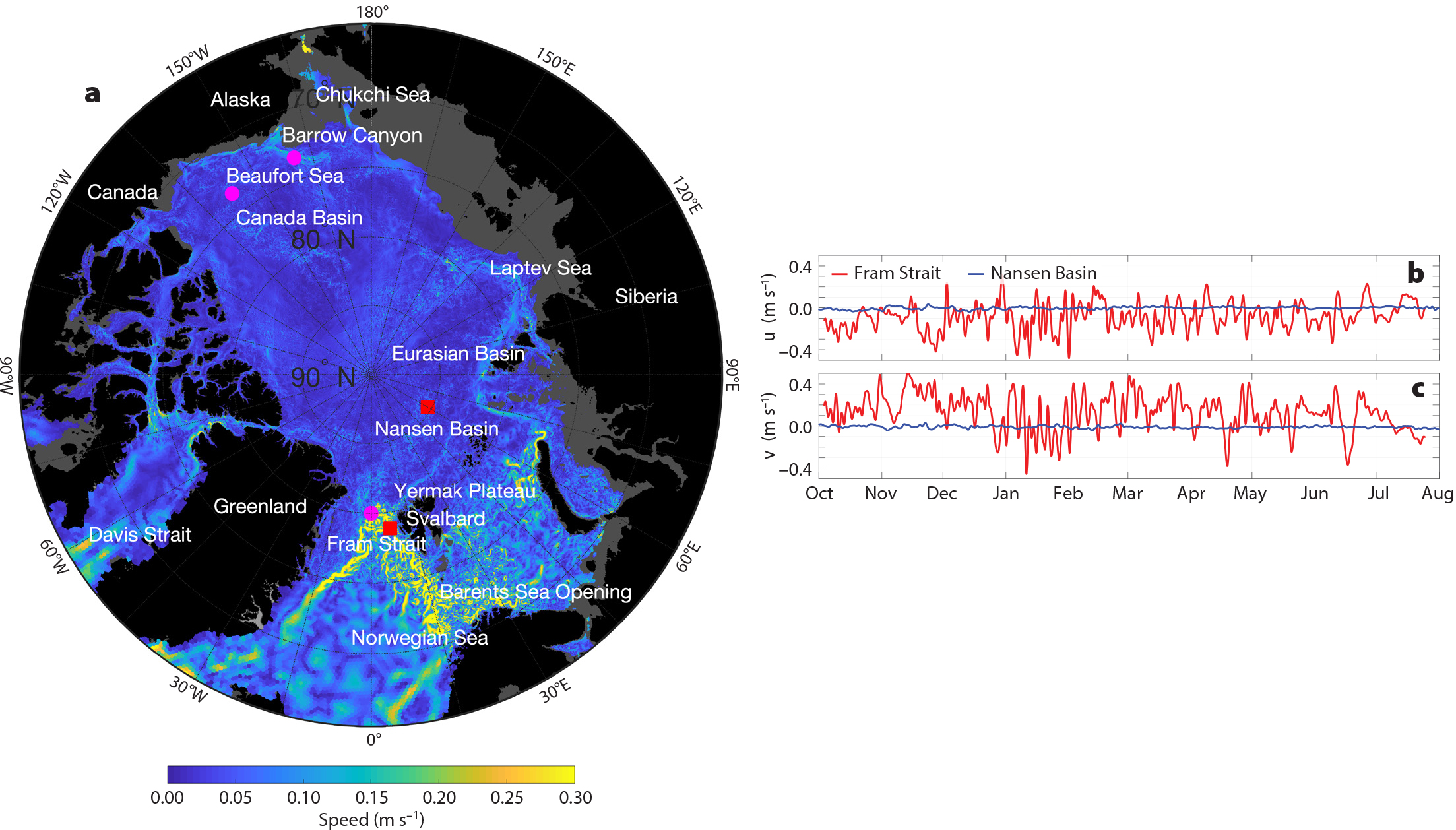
FIGURE 1. (a) Snapshot of current speed averaged over 50–100 m from 1 km numerical simulation of Wang et al. (2020) on December 30, 2008. Note that the 1 km resolution region of the model starts at approximately 75°N in the Nordic Seas. Place names are labeled in white and indicate locations close to the bottom left of each label. Magenta dots mark the locations of the studies shown in Figure 2. For illustrative purposes, two time series of velocity are presented, one representative of very high and one of very low mesoscale variability: (b) eastward velocity [m s–1] and (c) northward velocity [m s–1] at mooring F4 in Fram Strait and mooring Nansen in the Nansen Basin, both marked by red squares in (a). The velocities are averaged over 50–100 m and lowpass filtered with a two-day cutoff. F4, at 78°50'N 7°E in 1,416 m water depth, and Nansen, at 85°18’N 60°E in 3,870 m water depth, have average eddy kinetic energies of 1.3*10–2 m2 s–2 and 6.7*10–5 m2 s–2, respectively. > High res figure

 

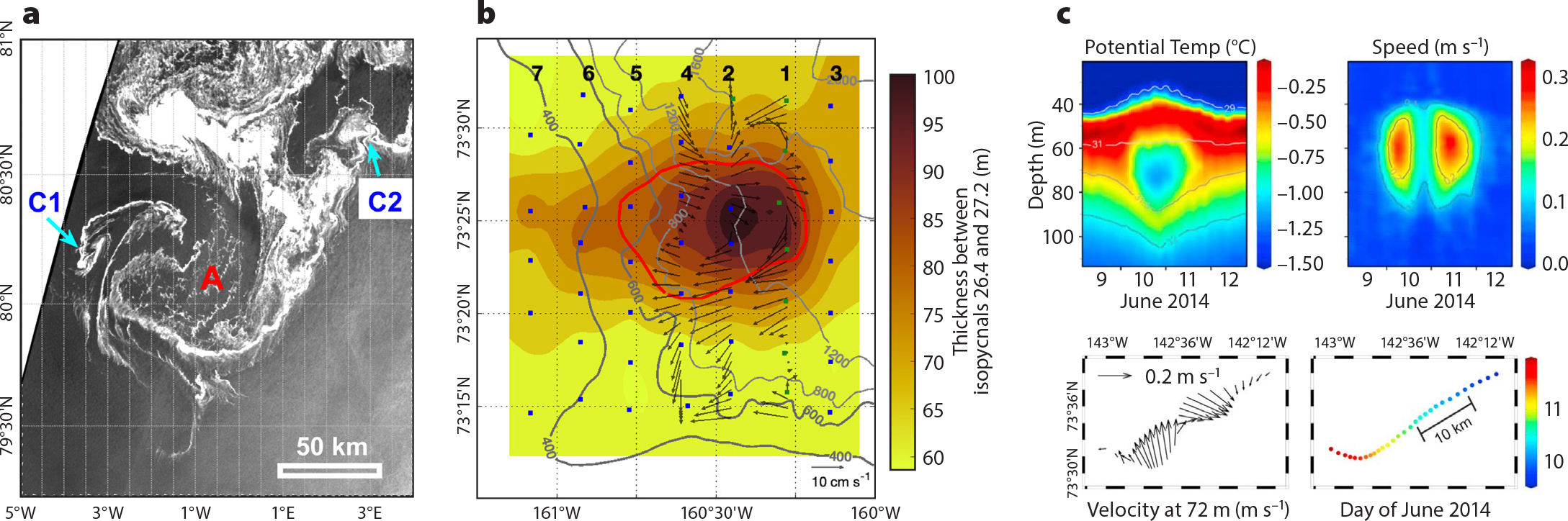
FIGURE 2. Examples from the literature show observations of eddies in the Arctic Ocean. (a) Synthetic aperture radar image of an anticyclone (A) and two cyclones (C1, C2) in the marginal ice zone of Fram Strait. White indicates sea ice, and dark gray indicates open water. (b) Map view of a shipboard hydrographic survey of an eddy of Pacific Water north of the Chukchi Sea. Color shows the thickness in m of the layer between the 26.4 kg m–3 and 27.2 kg m–3 isopycnals, and vectors show velocities from the vessel-mounted ADCP (scale vector in bottom right). (c) Time series of an eddy in the Canada Basin measured by an Ice-Tethered Profiler drifting over a typical upper halocline eddy. Top two panels show temperature/speed transects; bottom two panels provide map views of horizontal velocity/measurement date. (a) From Kozlov et al. (2020). (b) From Scott et al. (2019). (c) From Zhao et al. (2016), reprinted with permission from Wiley. The formatting of the x- and y-axis labels in (a) and (b) has been changed from the original. > High res figure

 

Baroclinic and barotropic instability of the northward-flowing West Spitsbergen Current on the eastern side of Fram Strait produces eddies, especially in winter when the boundary current is weakly stratified (von Appen et al., 2016, and references therein). The transfer rate of mean potential energy to eddy energy (i.e., baroclinic conversion with units of W m^–3) in this region has been estimated from observations (von Appen et al., 2016), and models show it to be higher than in most other regions of the Arctic (Wang et al., 2020). Tracking simulated eddies reveals that their lifetimes are on average 10 days in Fram Strait (Wekerle et al., 2020).

It is enlightening to consider different locations along the cyclonic Arctic Circumpolar Boundary Current (Aksenov et al., 2011). Northeast of Svalbard (near 30°E), Våge et al. (2016) showed a 25 km diameter mid-depth intensified anticyclonic (clockwise rotating in the Northern Hemisphere) eddy of Atlantic Water. This eddy highlights a likely mechanism of export of Atlantic Water and an associated heat flux to the Nansen Basin from the boundary current (Renner et al., 2018).

North of the Laptev Sea (near 125°E), mooring observations have shown eddies within and offshore of the boundary current with approximately one eddy per month passing this location (Pnyushkov et al., 2018). Some of the eddies have likely been advected from the western Nansen Basin or even from Fram Strait, while others may have formed from local baroclinic instability (Pnyushkov et al., 2018). Model simulations indicate that the continental slope region in the eastern Eurasian Basin features higher conversion from available potential energy to eddy kinetic energy than the interior of the Arctic basin (Wang et al., 2020).

Warm Pacific Water, which is lower in salinity and thus lighter than Atlantic Water, enters the Arctic Ocean from Bering Strait and crosses the shallow Chukchi Sea shelf. Upon exiting Barrow Canyon at the northeast edge of the shelf, it forms the eastward-​flowing Western Arctic Shelfbreak Current north of Alaska (Pickart, 2004) as well as the westward-​flowing Chukchi Slope Current north of the Chukchi Sea (Corlett and Pickart, 2017). Farther to the west, Pacific Water exiting Herald Canyon forms the eastward-flowing Chukchi Shelfbreak Current (Linders et al., 2017). Small (10–20 km diameter) anticyclonic eddies containing Pacific Water in their cores are commonly found in the Canada Basin (Manley and Hunkins, 1985, and Fine et al., 2018, and references therein) though at numbers much smaller than near the boundaries. These anticyclones are readily formed from the shelfbreak currents of the Chukchi and Beaufort Seas (e.g., Pickart et al., 2005; Scott et al., 2019; Figure 2b). The Western Arctic Shelfbreak Current was found to be baroclinically unstable (Spall et al., 2008; von Appen and Pickart, 2012), with mooring-​based baroclinic conversion rates near 152°W on the Beaufort slope varying seasonally with magnitudes close to those of Fram Strait.

The role of synoptic wind forcing as a source of mesoscale variability, in addition to eddies, was also studied extensively from the Beaufort slope array. It was found that atmosphere-to-ocean momentum transfer is more effective at intermediate (10%–70%) sea ice concentrations than in more consolidated pack ice or open water (Schulze and Pickart, 2012). On synoptic timescales, upwelling-favorable winds can bring relatively warm and nutrient-rich Atlantic Water across the shelf break and onto the shelf (Pickart et al., 2013). Conversely, downwelling-favorable winds are able to flush water that is rich in resuspended matter from the bottom boundary layer off the shelf (Dmitrenko et al., 2018; Foukal et al., 2019).

Most of the mooring measurements and ship-based observational studies in the Arctic are focused on the boundary currents. By contrast, knowledge of the variability in the deep basins is largely based on Ice-Tethered Profilers (ITPs). ITP surveys in the southern Canada Basin found significantly more anticyclonic than cyclonic eddies (e.g., Zhao et al., 2014). Normally, cyclones and anticyclones occur in roughly similar numbers in the ocean. The deviation from this pattern in the Beaufort Sea has been linked to the fact that cyclones tend to occur at the surface, while anticyclones are generally subsurface features. The associated surface velocities presumably lead to a relatively strong ice-ocean drag that spins down the cyclones without a comparable effect on anticyclones (Chao and Shaw, 1996).

Zhao and Timmermans (2015) identified three types of eddies in the Canada Basin: shallow eddies, mid-depth double core eddies, and deep eddies (Figure 2c shows an example of a shallow eddy). The radii of observed eddies tend to be centered at 7 km and 4 km in the Canada Basin and 4.5 km in the Eurasian sector of the Arctic Ocean (Zhao et al., 2014). These eddy length-scale estimates are in agreement with the comparatively smaller Rossby radius in the Eurasian Basin due to weaker stratification in the same depth range. Timmermans et al. (2008) proposed that some of the Beaufort Gyre eddies are produced from baroclinic instability of an upper ocean front near 78°N. Carpenter and Timmermans (2012) showed deep-reaching (>1,500 m) eddies in the weakly stratified Atlantic Water and deep water layers, while Bebieva and Timmermans (2019) identified the effects of eddies on double diffusion.

The studies discussed above provide a view of some of the Arctic Ocean observational programs that address mesoscale variability. The different programs are generally focused on specific geographical regions, depending on accessibility and national and institutional research priorities. They provide an incomplete view of Arctic mesoscale dynamics and activity. For an integral pan-Arctic view, we rely on information from numerical models, in particular from those with the sufficiently fine grids, on the order of ~1 km, that are needed to resolve most mesoscale processes in the deep Arctic Ocean. However, a quantitative evaluation of the models’ abilities to realistically reproduce the relevant processes as they occur in the ocean is important and requires comparison of metrics extracted from both models and observations. One such dynamically relevant parameter is eddy kinetic energy (EKE), which provides a measure of eddy activity and can readily be computed from both observations and numerical models. We provide an overview of mesoscale activity in the Arctic Ocean based on one such high-resolution numerical simulation and a compilation of mooring records collected over the past few decades by the international science community.

 

Data and Methods

We use two previously compiled comprehensive mooring current meter/acoustic Doppler current profiler (ADCP) databases (https://www.nature.com/​articles/​s41597-​020-​00578-z/​tables/3 and http://mespages.​univ-brest.fr/​~scott/​GMACMD/​gmacmd.html) that have been employed in past studies of tides (Baumann et al., 2020) and lee wave generation (Wright et al., 2014). We complemented these collections with more recent records as well as multiyear time series (as listed in a table at Pangaea; see von Appen et al., 2022) to more extensively investigate the temporal and spatial trends and variability in mesoscale activity.

We interpolated the depth-averaged eastward and northward velocities (u,v) to hourly values from 1980 to 2020. This was done separately for the depth ranges 50–100 m and 500–1,000 m, which roughly correspond to the halocline (upper Atlantic Water layer in western Eurasian Basin) and lower Atlantic Water/deep water layer, respectively, across most of the Arctic Ocean. In ice-covered waters, moorings cannot contain surface buoys, and upward-looking ADCPs cannot measure closer to the surface than 8% of their distance from the surface. Hence, no surface and near-surface observations exist. From the model (see below), we estimate that, on average, near-surface EKE values are 1.3 times larger than the 50–100 m average. We only considered observations over topography deeper than 50 m, given that mesoscale dynamics are fundamentally different on the shallow continental shelves. Redeployment locations in different years may vary by up to a few kilometers for operational reasons; hence, we clustered observations within 3 km of one another and considered them as a single mooring time series. In total, we have 212 deployment locations with an average duration of 2.4 years (ranging from 2 months to 18 years).

The quantities (u_mean,v_mean) are the velocities averaged over the full duration of the record. We then filtered the (u,v) with a fourth-order Butterworth filter to obtain: (u_lp,v_lp) = lowpass filtered with 30 day period cutoff, (u_bp, v_bp) = bandpass filtered with 2-day to 30-day cutoffs, and (u_hp, v_hp) = highpass filtered with 2-day cutoff. The 2-day cutoff is chosen to exclude tidal motions and inertial oscillations and the 30-day cutoff is chosen to exclude seasonal and interannual variability (comparable to, e.g., von Appen et al., 2016); hence, (u_bp, v_bp) allow us to concentrate on the mesoscale variability in the 2- to 30-day band. Data gaps smaller than the periods used for filtering were interpolated linearly, while larger data gaps were retained as missing values. We define the mean kinetic energy (MKE), low-​frequency kinetic energy (LKE), eddy kinetic energy (EKE), and high-frequency kinetic energy (HKE) as

 

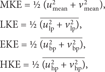where the mean is a temporal mean over the hourly values within, for example, a certain season or ice regime. In most cases, the sum of LKE, EKE, and HKE accounts for more than 90% of total kinetic energy (not shown). Kinetic energy in the ocean is a log-normally distributed quantity spanning many orders of magnitude, implying that the filtering does not artificially remove a lot of energy. We note that some eddies may have rotation-associated variability on periods longer than the bandpass cutoff. If these eddies translate through the domain, their signals may still be contained in the bandpass-filtered signal.

We also use a global simulation with the FESOM2 model that has a 1 km horizontal resolution in the Arctic Ocean (i.e., >75°N in the Nordic Seas, >65°N in the Bering Sea; Wang et al., 2020). The model is forced with the JRA55 atmospheric reanalysis product (Tsujino et al., 2018). The online model calculation of EKE is defined slightly differently (a quantification of all variability with periods less than a month; see equation 1 of Wang et al., 2020). We use this alternate definition in Figure 3, while we apply the bandpass-filtered EKE definition to daily model output for year 2009 (the only year for which daily output was saved) to calculate Figure 4d. The model does not contain tides. Hence, the HKE in the model is small and, on average, the online calculated EKE is less than two times larger than the bandpass-filtered EKE (Pangaea table). For a log-normally distributed quantity such as EKE, this constitutes good agreement. The third type of data we use is Advanced Microwave Scanning Radiometer (AMSR) satellite-​derived sea-​ice concentration provided at https://seaice.​uni-​bremen.de/​sea-​ice-​concentration/​amsre-​amsr2/ (Spreen et al., 2008), which ranges in time from 2002 to 2021.

 

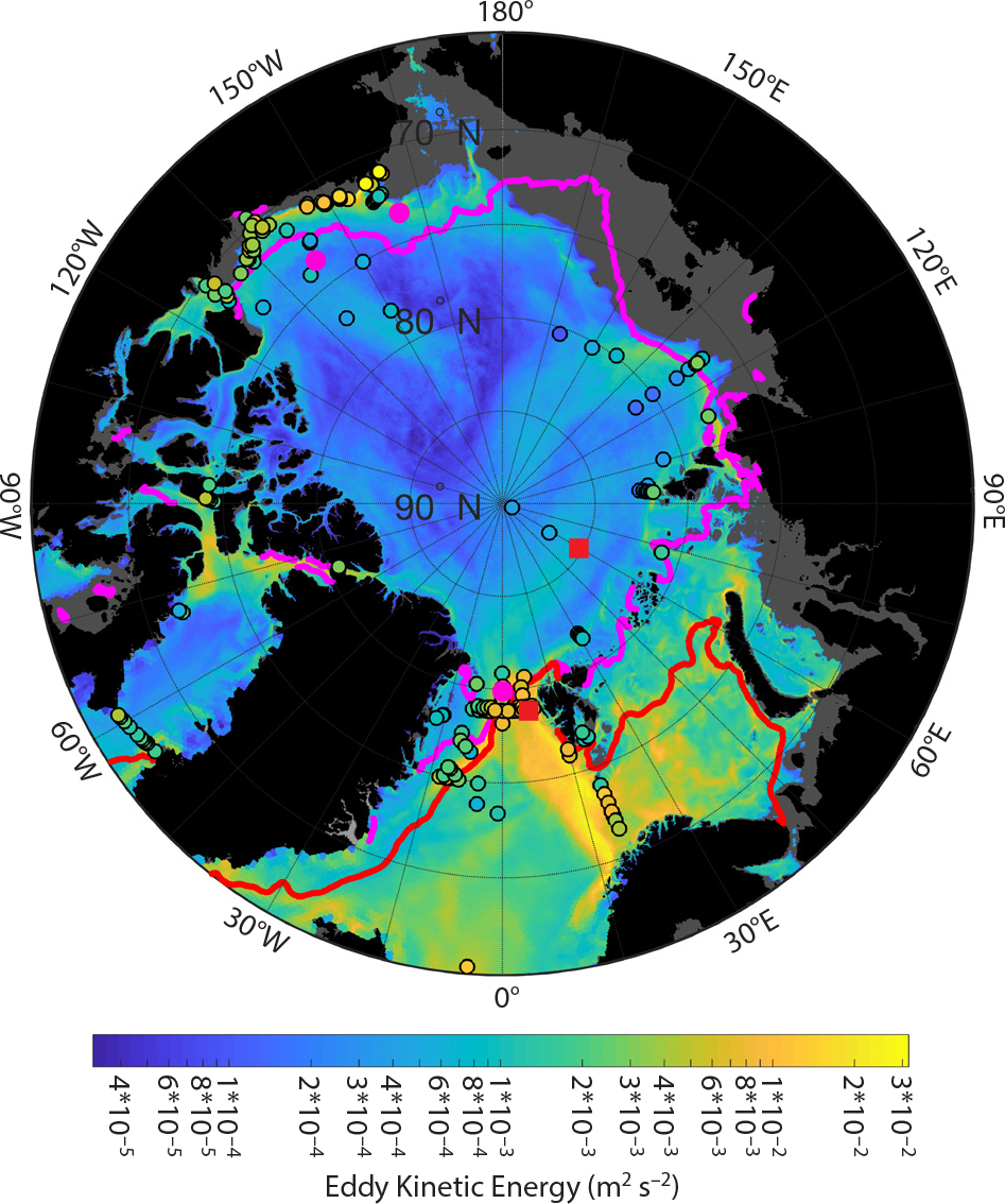
FIGURE 3. Map of 50–100 m eddy kinetic energy (EKE) [m2 s–2]. Values calculated from all available mooring records are shown as colored circles. Values corresponding to all variability with periods of less than 1 month taken from 1 km numerical simulation of Wang et al. (2020) are shown in the background. Note that moorings in very close spatial proximity partially overplot. A log10 scale is applied to the color bar. The 2002–2019 February (red) and August (magenta) mean sea ice edges (20% concentration) are also shown. Note that the summer ice edge has been located further north in the last decade. Land is shown in black and the shelves (model bathymetry <100 m depth) in dark gray. > High res figure

 

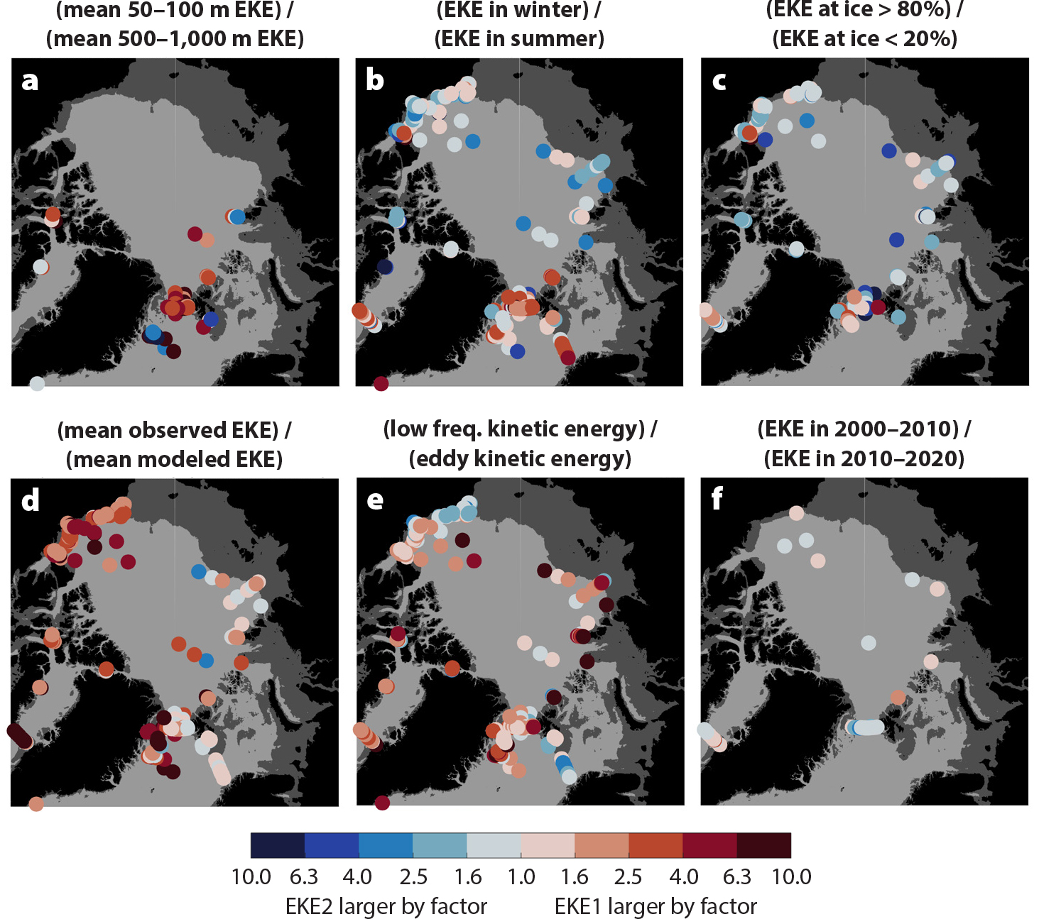
FIGURE 4. Maps of EKE ratios (EKE1/EKE2). (a) Shallow (50–100 m average) EKE divided by deep (500–1,000 m average) EKE. (b) Winter (January/February/March) EKE divided by summer (July/August/September) EKE. (c) Ice-covered EKE (>80% sea ice concentration at closest Advanced Microwave Scanning Radiometer (AMSR) grid point to the mooring location) divided by open water EKE (<20% sea-ice concentration). (d) Mooring-observed EKE divided by modeled EKE (Wang et al., 2020); here the model EKE is calculated from bandpass filtered daily mean time series in 2009. (e) Low-frequency kinetic energy (LKE) divided by EKE. The low-frequency (30-day lowpass filtered) kinetic energy includes seasonal and interannual variability. (f) EKE during 2000–2010 divided by EKE during 2010–2020. Except for (a), all EKEs are averages over 50–100 m. Land is shown in black, the shelves (<200 m depth) in dark gray, and the deep ocean (>200 m depth) in light gray; bathymetry is from IBCAOv3. > High res figure

 

Regional Hotspots and Temporal Variation of Mesoscale Variability in the Arctic Ocean

We present the 50–100 m averaged EKE calculated from all available mooring records as colored circles in Figure 3. The background color shows the numerical model-derived EKE of Wang et al. (2020). Consistent with the literature described above, our results identify the Beaufort shelf break, the Arctic Circumpolar Boundary Current, the western part of the Norwegian Sea, Barents Sea Opening, Fram Strait, and, to a lesser extent, the Yermak Plateau as hotspots of mesoscale variability. By comparison, the interior Canada Basin and, to a lesser extent, the Eurasian Basin are quiescent. These interior basin regions still contain eddies, but, as the EKE indicates, they are weaker (less energetic) and less frequent than in regions with higher EKE. EKE in the most energetic regions is almost 1,000 times larger than in the most quiescent regions. Note that this may also be affected by the fact that in the Atlantic inflow regions, the low stratification means that EKE in the 50–100 m depth range may be similar to (near-) surface variability, while in other regions with stronger stratification, there may be a steeper decline of the variability from the surface downward.

We now explore differences in the EKE (Figure 4) and try to explain some of them. EKE in the 50–100 m depth range is 1.5–10 times higher than EKE in the 500–1,000 m depth range (Figure 4a). Observations of 50–100 m EKE over topography shallower than 1,000 m are about an order of magnitude larger than EKE over topography deeper than 3,000 m (Pangaea table). In the Atlantic Water inflow regions (Barents Sea Opening, Fram Strait, western Nansen Basin), EKE in winter is 2–10 times higher than in summer (Figure 4b) and fall (Pangaea table). Presumably, the lack of dense ice covers in the inflow regions allows for the stronger atmospheric forcing in winter to drive mesoscale-band variability in the ocean directly. Additionally, baroclinic instability associated with convection may drive mesoscale-band variability in parts of the inflow regions. This is different along the eastern Siberian shelves and the Beaufort Sea where summer atmospheric forcing in ice-free conditions probably leads to stronger EKE, though the winter-​summer change is smaller than in the Atlantic inflow regions. Along the Alaskan slope, EKE is largest in fall (Pangaea table) when storm activity intensifies but full ice cover is not yet developed, consistent with the peak in momentum transfer from the atmosphere to the ocean under intermediate sea ice concentrations (Schulze and Pickart, 2012).

Sea ice cover leads to a reduction by a factor of 1.5–4 in EKE in most regions (Figure 4c) except for the parts of Fram and Davis Straits where sea ice cover is infrequent and its presence presumably represents especially strong flow events from the Arctic. The numerical model matches the observations well to within one order of magnitude (Figure 4d), with an average underestimation of slightly less than a factor of 2 (Pangaea table). However, the model predicts weaker variability in the western Arctic than observed.

EKE is larger (often by up to a factor of 10) than mean kinetic energy in most parts of the Arctic Ocean except for the Nansen Basin (Pangaea table). EKE accounts for up to half of total kinetic energy in the Beaufort Sea, while its share is smaller elsewhere (Pangaea table). However, low frequency kinetic energy, which includes seasonal and interannual variability, is 2–8 times larger than EKE in the boundary current north of Siberia and up to 2.5 times smaller than EKE along the western Beaufort slope (Figure 4e).

With regard to temporal change, the observations are limited, and most locations show differences between the decades 2000–2010 and 2010–2020 that are much less than the differences described above (Figure 4f). Fram Strait appears to show a small increase (~10%) in EKE, potentially linked to decreasing ice cover. Conversely, the eastern Arctic slope along Eurasia and the Beaufort slope regions show a small decrease by ~20%. This is counterintuitive, as an increase in the strength of the cyclonic boundary current has been observed in the eastern Eurasian Basin (Polyakov et al., 2020), which can be partially attributed to Arctic sea ice decline (Wang et al., 2019b). Note, however, that interdecadal changes may also be influenced by changes in the measurement configuration of long-term observations, especially due to the instrument type used and the vertical location and range of the measurements; hence, these conclusions should be considered tentative.

 

Impacts of Mesoscale Variability on Arctic Ocean Circulation, Sea Ice, and Biological Production

The mesoscale eddy field drives and/or affects a number of important processes in the Arctic. As boundary currents flow along the shelf break, they become baroclinically and/or barotropically unstable. The instabilities can result in the formation of eddies containing fluid from the boundary current, which thereby can flux mass and momentum into the basin (Spall et al., 2008). The associated loss of potential and kinetic energy suggests that the Western Arctic shelfbreak current will spin down over ~150 km in summer and ~1,400 km in winter (von Appen and Pickart, 2012). Also, in Fram Strait, the West Spitsbergen Current appears to lose mass offshore through eddy transport, mostly of Atlantic Water (von Appen et al., 2016), which feeds the recirculation in the strait (Hattermann et al., 2016).

The model of Nøst and Isachsen (2003) explains the Atlantic Water circulation as flow along f/H contours (where f is the Coriolis frequency and H is the water depth) that is due to the forcing associated with the integral of the wind component parallel to f/H contours. Conversely, the model of Spall (2013) provides a plausible way of explaining the cause for the Atlantic Water circulation: the horizontal eddy fluxes of salt from the Atlantic Water boundary current balance the vertical diffusion across the halocline. This sets the halocline depth, which in turn determines the boundary current velocity through thermal wind. In a warming climate with decreased ice cover and therefore more mechanical energy input from the atmosphere to the ocean, the vertical diffusion is expected to increase, resulting in a deeper halocline. Increased eddy generation would ensue from this additional available potential energy, and, through thermal wind, the Atlantic Water boundary current would increase in strength (Spall, 2013).

The Beaufort Gyre is a wind-driven, anticyclonic circulation that stores a substantial amount of freshwater (i.e., water with a lower salinity than, for instance, Atlantic Water). The wind-driven Ekman downwelling in the center of the Beaufort Gyre results in inclined isopycnals. These become baroclinically unstable, forming mesoscale eddies that counteract the downwelling through a residual mean circulation (Manucharyan and Spall, 2016; Meneghello et al., 2021). Recent studies suggest that changes in the wind-driven Beaufort Gyre strength are counteracted by the joint effect of ice-ocean stress coupling and mesoscale eddies (Meneghello et al., 2018; Wang et al., 2019a). As sea ice has retreated over the past two decades in the Canada Basin, additional wind energy has been input to the ocean, resulting in an increase in eddy activity in the Beaufort Gyre (Armitage et al., 2020).

Additionally, because they are intermittent, eddies lead to variations in water masses and the strength of stratification. Such changes impact horizontal and vertical mixing and can influence the amount of heat fluxed vertically across the halocline and available to melt sea ice. They can also alter the vertical nutrient flux necessary to sustain primary production (MacKinnon et al., 2021), as well as provide energy sources that locally increase turbulence.

Eddies modulate primary production and vertical carbon export from the productive layer in the Arctic Ocean in various ways. If eddies are not resolved explicitly (e.g., Schourup-Kristensen et al., 2018) their biogeochemical effects in ocean general circulation biogeochemistry models of the Arctic need to be parameterized, which is difficult in the absence of a complete knowledge of the relevant processes. Under-ice primary production is a key contributor to the total primary production in the Arctic Ocean (Jin et al., 2015). Because eddies can modulate sea ice concentration and distribution (see below), they may have a nonlinear effect on primary production in the Arctic Ocean. Unlike eddy permitting models, low resolution ocean biogeochemistry models fail to reproduce features such as the low surface nutrient concentrations in the Canada Basin (Jin et al., 2018), suggesting that eddies may be an important mechanism for establishing nutrient distribution. Watanabe et al. (2014) argued that shelfbreak mesoscale eddies are vital in transporting biomass from the wide Arctic shelves to the deep basins where it can be sequestered by sinking (i.e., the biological carbon pump). Likewise, eddies can carry resuspended matter from the shelves to the basins, e.g., in eastern Fram Strait (Koenig et al., 2018).

Several dedicated field (as well as numerical modeling) programs designed to study the differences in ecology and biogeochemistry inside and outside of mesoscale eddies in lower latitudes have been carried out over recent decades. Among other findings, this has led to the conclusion that anticyclones (cyclones) with downwelling (upwelling) in their centers typically exhibit less (more) primary production than surrounding waters. The number of similar studies in the Arctic is small (e.g., Llinás et al., 2009; O’Brien et al., 2013; Nishino et al., 2018, and references therein) largely because of the logistical challenges of working in ice-covered waters, the short phytoplankton growth season, and the small eddy scales of several kilometers.

Consolidated sea ice dampens eddy kinetic energy by reducing the atmosphere-​ocean momentum transfer that drives part of the mesoscale variability, for example, along Arctic shelf breaks (Figure 4c). Conversely, in the marginal ice zone, the atmosphere to ocean momentum transfer changes with the presence/absence of sea ice. Thus, strong sea ice concentration gradients may represent an approximate step change in regions experiencing heat loss and wind mixing (both enhanced on the open water side). This may also set up density fronts in the upper ocean that become unstable and form mesoscale (and submesoscale) eddies.

Detection of eddies from space is largely limited in the Arctic Ocean by the presence of sea ice and the eddies’ small scales. In the open water, however, satellite altimetry can be used to detect large eddies (Kubryakov et al., 2021). von Appen et al. (2016) demonstrated that along-track altimetry data can be used in the non-ice-covered ocean to obtain EKE estimates consistent with mooring-based estimates. Sea ice, especially at low to intermediate concentrations (i.e., in the marginal ice zone), acts as an approximate passive surface tracer similar to biofilms/oil and surface drifters. Hence, satellites may show narrow streaks of high sea ice concentration that enable us to visualize surface divergence and strain fields. These signatures can be readily detected by satellite synthetic aperture radar (SAR; e.g., Figure 2a). From sequential images, surface velocity (Kozlov et al., 2020) and vorticity (Cassianides et al., 2021) can be inferred. These SAR signatures have been used to guide in situ sampling campaigns targeting mesoscale eddies (e.g., Johannessen et al., 1987) and submesoscale fronts (von Appen et al., 2018) in the marginal ice zone. The differential advection of sea ice by the mesoscale flow field in the marginal ice zone may impact regional sea ice melt and formation rates by either exposing or sheltering sea ice from warm ocean water (Horvat et al., 2016).

 

Concluding Remarks

Based on the insights presented above, we can speculate about how mesoscale variability might change in the future Arctic Ocean with progressing sea ice decline and Atlantification (Polyakov et al., 2017; and see sidebar by Pnyushkov and Polyakov, 2022, in this issue). Areas that are ice-free in winter, or have low ice concentrations, are associated with large EKE in winter (Figure 4b), suggesting that a decrease in winter sea ice extent in a warming climate may facilitate more eddy generation. This change may particularly apply to the continental slopes, which are now often subject to summertime melt. For example, the eddy formation mechanism of Timmermans et al. (2008) requires winds blowing parallel to a frontal jet (resulting in jet acceleration and subsequent destabilization). Such a mechanism is much more likely to occur in low ice conditions. Spin-up of the boundary current will also be associated with an increase in available potential energy and thus baroclinic instability. All these mechanisms would lead to more eddies in the Arctic Ocean.

Other interesting investigations that could be based on the mooring records used here include calculation of the number of individual eddies passing by each of the mooring sites and detection of mesoscale variability in the accompanying temperature records. It would also be worthwhile to investigate more carefully the lifetimes of eddies in different locations, and, considering their translation speeds, how far they propagate through the Arctic Ocean. The curvature of topographic corners along isobaths, in combination with the inertia in boundary currents, is predestined to lead to eddy shedding. Hence, the relation between the curvature of the topography and the frequency of eddies and the EKE could also be investigated to determine, among other things, their basin-wide relevance. These investigations might uncover important aspects of Arctic Ocean eddies that are presently unknown.

Finally, additional studies will help to improve our understanding of present and future mesoscale variability in the Arctic Ocean, especially in the central basins, including its effect on physical-​biological coupling and sea ice. Field efforts should include observations with moorings and ice-based platforms and also make use of the novel under-ice capabilities of gliders and Argo floats. Whenever possible, these should be done in tandem with idealized and/or realistic high-​resolution numerical modeling.

 

Acknowledgments

We thank all the scientists who collected and analyzed the observations that we use in this study, especially Eugenio Ruiz-Castillo for the use of unpublished data. We also thank the two anonymous reviewers. The full metadata of the mooring records and the calculated kinetic energies at the mooring locations are available as a table at Pangaea (von Appen et al., 2022).

von Appen, W.-J., T.M. Baumann, M. Janout, N. Koldunov, Y.-D. Lenn, R.S. Pickart, R.B. Scott, and Q. Wang. 2022. Eddies and the distribution of eddy kinetic energy in the Arctic Ocean. Oceanography 35(3–4):42–51, https://doi.org/10.5670/oceanog.2022.122.

Aksenov, Y., V.V. Ivanov, A.J.G. Nurser, S. Bacon, I.V. Polyakov, A.C. Coward, A.C. Naveira-Garabato, and A. Beszczynska-Möller. 2011. The Arctic Circumpolar Boundary Current. Journal of Geophysical Research 116(C9), https://doi.org/​10.1029/2010JC006637.
1. Armitage, T.W.K., G.E. Manucharyan, A.A. Petty, R. Kwok, and A.F. Thompson. 2020. Enhanced eddy activity in the Beaufort Gyre in response to sea ice loss. Nature Communications 11:761, https://doi.org/​10.1038/s41467-020-14449-z.
2. Baumann, T.M., I.V. Polyakov, L. Padman, S. Danielson, I. Fer, M. Janout, W. Williams, and A.V. Pnyushkov. 2020. Arctic tidal current atlas. Scientific Data 7:275, https://doi.org/10.1038/s41597-020-00578-z.
3. Bebieva, Y., and M.-L. Timmermans. 2019. Double-diffusive layering in the Canada Basin: An explanation of along-layer temperature and salinity gradients. Journal of Geophysical Research: Oceans 124(1):723–735, https://doi.org/​10.1029/​2018JC014368.
4. Carpenter, J.R., and M.L. Timmermans. 2012. Deep mesoscale eddies in the Canada Basin, Arctic Ocean. Geophysical Research Letters 39(20), https://doi.org/10.1029/2012GL053025.
5. Cassianides, A., C. Lique, and A. Korosov. 2021. Ocean eddy signature on SAR-derived sea ice drift and vorticity. Geophysical Research Letters 48(6):e2020GL092066, https://doi.org/​10.1029/2020GL092066.
6. Chao, S.Y., and P.T. Shaw. 1996. Initialization, asymmetry, and spindown of Arctic eddies. Journal of Physical Oceanography 26(10):2,076–2,092, https://doi.org/10.1175/1520-0485(1996)026​<2076:IAASOA>​2.0.CO;2.
7. Corlett, W.B., and R.S. Pickart. 2017. The Chukchi slope current. Progress in Oceanography 153:50–65, https://doi.org/​10.1016/j.pocean.2017.04.005.
8. Dmitrenko, I.A., S.A. Kirillov, P.G. Myers, A. Forest, B. Tremblay, J.V. Lukovich, Y. Gratton, S. Rysgaard, D.G. Barber, and M.-L. Timmermans. 2018. Wind-forced depth-dependent currents over the eastern Beaufort Sea continental slope: Implications for Pacific water transport. Elementa: Science of the Anthropocene 6:66, https://doi.org/10.1525/elementa.321.
9. Fine, E.C., J.A. MacKinnon, M.H. Alford, and J.B. Mickett. 2018. Microstructure observations of turbulent heat fluxes in a warm-core Canada Basin eddy. Journal of Physical Oceanography 48(10):2,397–2,418, https://doi.org/​10.1175/​JPO-D-18-0028.1.
10. Foukal, N.P., R.S. Pickart, G.W.K. Moore, and P. Lin. 2019. Shelfbreak downwelling in the Alaskan Beaufort Sea. Journal of Geophysical Research: Oceans 124(10):7,201–7,225, https://doi.org/​10.1029/2019JC015520.
11. Gnanadesikan, A. 1999. A simple predictive model for the structure of the oceanic pycnocline. Science 283(5410):2,077–2,079, https://doi.org/​10.1126/science.283.5410.2077.
12. Hattermann, T., P.E. Isachsen, W.-J. von Appen, J. Albretsen, and A. Sundfjord. 2016. Eddy-driven recirculation of Atlantic Water in Fram Strait. Geophysical Research Letters 43(7):3,406–3,414, https://doi.org/10.1002/2016GL068323.
13. Horvat, C., E. Tziperman, and J.-M. Campin. 2016. Interaction of sea ice floe size, ocean eddies, and sea ice melting. Geophysical Research Letters 43(15):8,083–8,090, https://doi.org/​10.1002/​2016GL069742.
14. Jin, M., E.E. Popova, J. Zhang, R. Ji, D. Pendleton, Ø. Varpe, A. Yool, and Y.J. Lee. 2015. Ecosystem model intercomparison of under-ice and total primary production in the Arctic Ocean. Journal of Geophysical Research: Oceans 121(1):934–948, https://doi.org/10.1002/2015JC011183.
15. Jin, M., C. Deal, W. Maslowski, P. Matrai, A. Roberts, R. Osinski, Y.J. Lee, M. Frants, S. Elliott, N. Jeffery, and others. 2018. Effects of model resolution and ocean mixing on forced ice-ocean physical and biogeochemical simulations using global and regional system models. Journal of Geophysical Research: Oceans 123(1):358–377, https://doi.org/​10.1002/2017JC013365.
16. Johannessen, O.M., J.A. Johannessen, E. Svendsen, R.A. Shuchman, W.J. Campbell, and E. Josberger. 1987. Ice-edge eddies in the Fram Strait marginal ice zone. Science 236(4800):427–429, https://doi.org/​10.1126/​science.236.4800.427.
17. Koenig, Z., A. Meyer, C. Provost, N. Sennéchael, A. Sundfjord, L. Beguery, M. Athanase, and J.-C. Gascard. 2018. Cooling and freshening of the West Spitsbergen Current by shelf-origin cold core lenses. Journal of Geophysical Research: Oceans 123(11):8,299–8,312, https://doi.org/​10.1029/​2018JC014463.
18. Kozlov, I.E., E.V. Plotnikov, and G.E. Manucharyan. 2020. Brief communication: Mesoscale and submesoscale dynamics in the marginal ice zone from sequential synthetic aperture radar observations. The Cryosphere 14(9):2,941–2,947, https://doi.org/​10.5194/tc-14-2941-2020.
19. Kubryakov, A.A., I.E. Kozlov, and G.E. Manucharyan. 2021. Large mesoscale eddies in the Western Arctic Ocean from satellite altimetry measurements. Journal of Geophysical Research: Oceans 126(5):e2020JC016670, https://doi.org/​10.1029/2020JC016670.
20. Lenn, Y.-D., I. Fer, M.-L. Timmermans, and J.A. MacKinnon. 2021. Mixing in the Arctic Ocean. Pp. 275–279 in Ocean Mixing: Drivers, Mechanisms, and Impacts. M. Meredith and A. Naveira Garabato, eds, https://doi.org/10.1016/B978-0-12-821512-8.00018-9.
21. Linders, J., R.S. Pickart, G. Björk, and G.W.K. Moore. 2017. On the nature and origin of water masses in Herald Canyon, Chukchi Sea: Synoptic surveys in summer 2004, 2008, and 2009. Progress in Oceanography 159:99–114, https://doi.org/10.1016/​j.pocean.2017.09.005.
22. Llinás, L., R.S. Pickart, J.T. Mathis, and S.L. Smith. 2009. Zooplankton inside an Arctic Ocean cold-core eddy: Probable origin and fate. Deep Sea Research Part II 56(17):1,290–1,304, https://doi.org/​10.1016/​j.dsr2.2008.10.020.
23. MacKinnon, J., H. Simmons, J. Hargrove, J. Thomson, T. Peacock, M. Alford, B. Barton, S. Boury, S. Brenner, N. Couto, and others. 2021. A warm jet in a cold ocean. Nature Communications 12:2418, https://doi.org/10.1038/s41467-021-22505-5.
24. Manley, T.O., and K. Hunkins. 1985. Mesoscale eddies of the Arctic Ocean. Journal of Geophysical Research 90(C3), https://doi.org/10.1029/JC090iC03p04911.
25. Manucharyan, G.E., and M.A. Spall. 2016. Wind-driven freshwater buildup and release in the Beaufort Gyre constrained by mesoscale eddies. Geophysical Research Letters 43(1):273–282, https://doi.org/10.1002/2015GL065957.
26. Meneghello, G., J. Marshall, J.-M. Campin, E. Doddridge, and M.-L. Timmermans. 2018. The ice-ocean governor: Ice-ocean stress feedback limits Beaufort gyre spin-up. Geophysical Research Letters 45(20):11,293–11,299, https://doi.org/​10.1029/2018GL080171.
27. Meneghello, G., J. Marshall, C. Lique, P.E. Isachsen, E. Doddridge, J.-M. Campin, H. Regan, and C. Talandier. 2021. Genesis and decay of mesoscale baroclinic eddies in the seasonally ice-​covered interior Arctic Ocean. Journal of Physical Oceanography 51(1):115–129, https://doi.org/10.1175/JPO-D-20-0054.1.
28. Nishino, S., Y. Kawaguchi, A. Fujiwara, T. Shiozaki, M. Aoyama, N. Harada, and T. Kikuchi. 2018. Biogeochemical anatomy of a cyclonic warm-core eddy in the Arctic Ocean. Geophysical Research Letters 45(20):11,284–11,292, https://doi.org/​10.1029/2018GL079659.
29. Nøst, O.A., and P.E. Isachsen. 2003. The large-scale time-mean ocean circulation in the Nordic Seas and Arctic Ocean estimated from simplified dynamics. Journal of Marine Research 61(2):175–210, https://doi.org/10.1357/002224003322005069.
30. Nurser, A.J.G., and S. Bacon. 2014. The Rossby radius in the Arctic Ocean. Ocean Science 10(6):967–975, https://doi.org/10.5194/os-10-967-2014.
31. O’Brien, M.C., H. Melling, T.F. Pedersen, and R.W. Macdonald. 2013. The role of eddies on particle flux in the Canada Basin of the Arctic Ocean. Deep Sea Research Part I 71:1–20, https://doi.org/​10.1016/​j.dsr.2012.10.004.
32. Pickart, R.S. 2004. Shelfbreak circulation in the Alaskan Beaufort Sea: Mean structure and variability. Journal of Geophysical Research 109(C4), https://doi.org/10.1029/2003JC001912.
33. Pickart, R.S., T.J. Weingartner, L.J. Pratt, S. Zimmermann, and D.J. Torres. 2005. Flow of Winter-transformed Pacific Water into the Western Arctic. Deep Sea Research Part II 52(24–26):3,175–3,198, https://doi.org/​10.1016/j.dsr2.2005.10.009.
34. Pickart, R.S., M.A. Spall, and J.T. Mathis. 2013. Dynamics of upwelling in the Alaskan Beaufort Sea and associated shelf-basin fluxes. Deep Sea Research Part I 76:35–51, https://doi.org/10.1016/​j.dsr.2013.01.007.
35. Pnyushkov, A., I. Polyakov, L. Padman, and A.T. Nguyen. 2018. Structure and dynamics of mesoscale eddies over the Laptev Sea continental slope in the Arctic Ocean. Ocean Science, https://doi.org/10.5194/os-2018-22.
36. Pnyushkov, A.V., and I.V. Polyakov. 2022. Nansen and Amundsen Basins Observational System (NABOS): Contributing to understanding changes in the Arctic. Oceanography 35(3–4):90–93, https://doi.org/10.5670/oceanog.2022.104.
37. Polyakov, I.V., A.V. Pnyushkov, M.B. Alkire, I.M. Ashik, T.M. Baumann, E.C. Carmack, I. Goszczko, J. Guthrie, V.V. Ivanov, T. Kanzow, and others. 2017. Greater role for Atlantic inflows on sea-ice loss in the Eurasian Basin of the Arctic Ocean. Science 356(6335):285–291, https://doi.org/10.1126/science.aai8204.
38. Polyakov, I.V., T.P. Rippeth, I. Fer, T.M. Baumann, E.C. Carmack, V.V. Ivanov, M. Janout, L. Padman, A.V. Pnyushkov, and R. Rember. 2020. Intensification of near-surface currents and shear in the eastern Arctic Ocean. Geophysical Research Letters 47(16): e2020GL089469, https://doi.org/​10.1029/​2020GL089469.
39. Porter, M., S.F. Henley, A. Orkney, H.A. Bouman, B. Hwang, E. Dumont, E.J. Venables, and F. Cottier. 2020. A polar surface eddy obscured by thermal stratification. Geophysical Research Letters 47(6):e2019GL086281, https://doi.org/​10.1029/2019GL086281.
40. Renner, A.H.H., A. Sundfjord, M.A. Janout, R.B. Ingvaldsen, A. Beszczynska-Möller, R.S. Pickart, and M.D. Pérez-Hernández. 2018. Variability and redistribution of heat in the Atlantic Water boundary current north of Svalbard. Journal of Geophysical Research: Oceans 123(9):6,373–6,391, https://doi.org/10.1029/2018JC013814.
41. Schourup-Kristensen, V., C. Wekerle, D. Wolf-Gladrow, and C. Völker. 2018. Arctic Ocean biogeochemistry in the high resolution FESOM 1.4-REcoM2 model. Progress in Oceanography 168:65–81, https://doi.org/​10.1016/j.pocean.2018.09.006.
42. Schulze, L.M., and R.S. Pickart. 2012. Seasonal variation of upwelling in the Alaskan Beaufort Sea: Impact of sea ice cover. Journal of Geophysical Research 117(C6), https://doi.org/​10.1029/​2012JC007985.
43. Scott, R.M., R.S. Pickart, P. Lin, A. Münchow, M. Li, D.A. Stockwell, and J.A. Brearley. 2019. Three-dimensional structure of a cold-core Arctic eddy interacting with the Chukchi Slope Current. Journal of Geophysical Research: Oceans 124(11):8,375–8,391, https://doi.org/​10.1029/2019JC015523.
44. Spall, M.A., R.S. Pickart, P.S. Fratantoni, and A.J. Plueddemann. 2008. Western Arctic shelfbreak eddies: Formation and transport. Journal of Physical Oceanography 38(8):1,644–1,668, https://doi.org/​10.1175/2007JPO3829.1.
45. Spall, M.A. 2013. On the circulation of Atlantic Water in the Arctic Ocean. Journal of Physical Oceanography 43:(11):2,352–2,371, https://doi.org/​10.1175/​JPO-D-13-079.1.
46. Spreen, G., L. Kaleschke, and G. Heygster. 2008. Sea ice remote sensing using AMSR-E 89-GHz channels. Journal of Geophysical Research: Oceans 113(C2), https://doi.org/​10.1029/2005JC003384.
47. Timmermans, M.-L., J. Toole, A. Proshutinsky, R. Krishfield, and A. Plueddemann. 2008. Eddies in the Canada Basin, Arctic Ocean, observed from Ice-tethered Profilers. Journal of Physical Oceanography 38:133–145, https://doi.org/​10.1175/2007JPO3782.1.
48. Tsujino, H., S. Urakawa, H. Nakano, R. Small, W. Kim, S. Yeager, and D. Yamazaki. 2018. JRA-55 based surface dataset for driving ocean–sea-ice models (JRA55-do). Ocean Modelling 130:79–139, https://doi.org/10.1016/j.ocemod.2018.07.002.
49. Våge, K., R.S. Pickart, V. Pavlov, P. Lin, D.J. Torres, R.B. Ingvaldsen, A. Sundfjord, and A. Proshutinsky. 2016. The Atlantic Water boundary current in the Nansen Basin: Transport and mechanisms of lateral exchange. Journal of Geophysical Research 121(9):6,946–6,960, https://doi.org/​10.1002/2016JC011715.
50. von Appen, W.-J., and R.S. Pickart. 2012. Two configurations of the Western Arctic Shelfbreak Current in summer. Journal of Physical Oceanography 42(3):329–351, https://doi.org/​10.1175/JPO-D-11-026.1.
51. von Appen, W.-J., U. Schauer, T. Hattermann, and A. Beszczynska-Möller. 2016. Seasonal cycle of mesoscale instability of the West Spitsbergen Current. Journal of Physical Oceanography 46(4):1,231–1,254, https://doi.org/​10.1175/​JPO-D-15-0184.1.
52. von Appen, W.-J., C. Wekerle, L. Hehemann, V. Schourup-Kristensen, C. Konrad, and M. Iversen. 2018. Observations of a submesoscale cyclonic filament in the marginal ice zone. Geophysical Research Letters 45(12):6,141–6,149, https://doi.org/​10.1029/​2018GL077897.
53. von Appen, W.-J., T. Baumann, M. Janout, N. Koldunov, Y.-D. Lenn, R.S. Pickart, R.B. Scott, and Q. Wang. 2022. Eddy kinetic energy in the Arctic Ocean from moored velocity observations. PANGAEA, https://doi.org/10.1594/PANGAEA.941165.
54. Wang, Q., J. Marshall, J. Scott, G. Meneghello, S. Danilov, and T. Jung. 2019a. On the feedback of ice–ocean stress coupling from geostrophic currents in an anticyclonic wind regime over the Beaufort Gyre. Journal of Physical Oceanography 49(2):369–383, https://doi.org/​10.1175/JPO-D-18-0185.1.
55. Wang, Q., C. Wekerle, S. Danilov, D. Sidorenko, N. Koldunov, D. Sein, B. Rabe, and T. Jung. 2019b. Recent sea ice decline did not significantly increase the total liquid freshwater content of the Arctic Ocean. Journal of Climate 32(1):15–32, https://doi.org/10.1175/JCLI-D-18-0237.1.
56. Wang, Q., N.V. Koldunov, S. Danilov, D. Sidorenko, C. Wekerle, P. Scholz, I.L. Bashmachnikov, and T. Jung. 2020. Eddy kinetic energy in the Arctic Ocean from a global simulation with a 1-km Arctic. Geophysical Research Letters 47(14):e2020GL088550, https://doi.org/​10.1029/2020GL088550.
57. Warren, B., and C. Wunsch. 1981. Evolution of Physical Oceanography: Scientific Surveys in Honor of Henry Stommel. MIT Press, 664p.
58. Watanabe, E., J. Onodera, N. Harada, M.C. Honda, K. Kimoto, T. Kikuchi, S. Nishino, K. Matsuno, A. Yamaguchi, A. Ishida, and others. 2014. Enhanced role of eddies in the Arctic marine biological pump. Nature Communications 5:3950, https://doi.org/10.1038/ncomms4950.
59. Wekerle, C., T. Hattermann, Q. Wang, L. Crews, W.-J. von Appen, and S. Danilov. 2020. Properties and dynamics of mesoscale-eddies in the Fram Strait from a comparison between two high-resolution ocean-sea ice models. Ocean Science 16:1,225–1,246, https://doi.org/10.5194/os-16-1225-2020.
60. Wright, C.J., R.B. Scott, P. Ailliot, and D. Furnival. 2014. Lee wave generation rates in the deep ocean. Geophysical Research Letters 41(7):2,434–2,440, https://doi.org/10.1002/2013GL059087.
61. Zhao, M., M.-L. Timmermans, S. Cole, R. Krishfield, A. Proshutinsky, and J. Toole. 2014. Characterizing the eddy field in the Arctic Ocean halocline. Journal of Geophysical Research: Oceans 119(12):8,800–8,817, https://doi.org/​10.1002/​2014JC010488.
62. Zhao, M., and M.-L. Timmermans. 2015. Vertical scales and dynamics of eddies in the Arctic Ocean’s Canada Basin. Journal of Geophysical Research 120(12):8,195–8,209, https://doi.org/​10.1002/2015JC011251.
63. Zhao, M., M.-L. Timmermans, S. Cole, R. Krishfield, and J. Toole. 2016. Evolution of the eddy field in the Arctic Ocean’s Canada Basin, 2005–2015. Geophysical Research Letters 43(15):8,106–8,114, https://doi.org/10.1002/2016GL069671.

This is an open access article made available under the terms of the Creative Commons Attribution 4.0 International License (https://creativecommons.org/licenses/by/4.0/), which permits use, sharing, adaptation, distribution, and reproduction in any medium or format as long as users cite the materials appropriately, provide a link to the Creative Commons license, and indicate the changes that were made to the original content. Images, animations, videos, or other third-party material used in articles are included in the Creative Commons license unless indicated otherwise in a credit line to the material. If the material is not included in the article’s Creative Commons license, users will need to obtain permission directly from the license holder to reproduce the material.