
Full Text
Soundscape Defined
Sound travels further through water than light and is one reason why many marine animals use sound to communicate and gain information about their surroundings. Scientists collect recordings of these underwater sounds to gain information on species’ habitat use, abundance, distribution, density, and behavior. In waters where visibility is severely limited or access is difficult or cost-intensive, passive acoustic monitoring is a particularly important technique for obtaining such biological information over space and time.
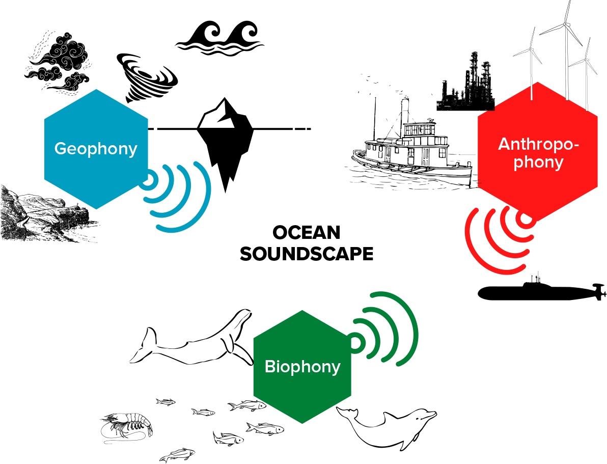
The “soundscape” of an ecosystem is defined as the characterization of all the acoustic sources present in a certain place (Wilford et al., 2021). A soundscape includes three fundamental sound source types (Figure 1): (1) anthropophony, or sounds associated with human activity; (2) biophony, or sounds produced by animals; and (3) geophony, or sounds generated by physical events such as waves, earthquakes, or rain (Pijanowski et al., 2011). Studying soundscapes can provide biological information for a specific habitat, which could then be linked to ecosystem health status and other bioindicators. This information can be used to monitor the habitat over time, allowing for rapid detection of habitat degradation, such as in response to human-driven events.
|
|
Soundscape Data Acquisition
Acoustic recordings can be collected using devices that are either fixed to the ocean floor or floating/navigating in the water column; by stations cabled to a land-based laboratory; or by instruments towed from boats (i.e., hydrophones) or attached to animals (i.e., bio-loggers). New technologies permit long deployments (months) that generate large amounts of acoustic data. Analyses of these data are very labor and time intensive, so automation is highly desirable.
Soundscape Analyses
Because the study of underwater soundscapes is relatively new, there is not yet a standardized way of processing acoustic data (Wilford et al., 2021). Thus, given the variety of instruments, mooring types, and deployment settings available, it can be challenging to compare results between different data sets. However, some initiatives, like the International Quiet Ocean Experiment (IQOE), are creating standards for underwater sound processing.
When analyzing acoustic habitats, different approaches can be considered. Common examples include the detection and quantification of specific events or the calculation of acoustic indices, which are summary statistics that describe the distribution of acoustic energy and can sometimes be correlated with certain biological or ecological habitat properties. Apart from classical acoustic indices, sound ecological indices could reveal the status of marine ecosystems, but they require previous knowledge about each sound type and its characteristics. One common approach to visualizing the soundscape is to use a spectrogram, a visual representation of a sound’s intensity and frequency over time. A spectrogram allows identification of interesting acoustic events and their timing, even for sounds outside the human hearing range.
Noise Pollution
Over the last many decades, human activities at sea such as pile driving, dredging, or shipping have increased, contributing to and sometimes dominating underwater sound levels. When anthropophony masks biophony, marine animals that rely on sound to detect predators or prey, to find or communicate with mates or offspring, and/or to navigate can be harmed (Duarte et al., 2021). Thus, it is important to describe and record the soundscapes of places that are currently less and more disturbed to quantify current noise levels. Knowledge of these “baselines” will enable us to measure additional human-driven degradation to the oceanic soundscape and the resulting impact on marine life.
Jacques Cousteau’s first impression of the ocean was that it was silent. We now know it has always been filled with natural sounds. In 2008, the European Marine Strategy Framework Directive (MSFD) established that low underwater sound levels are one descriptor of a Good Environmental Status (GES) (MSFD 2008/56/EC), even though there is still no common description of an acoustic GES. On the other side of the Atlantic Ocean, and in the Southern Hemisphere, Colombia’s National Environmental Licensing Authority (ANLA), in charge of environmental regulations for infrastructure projects, stipulated in articles 2 and 3 of decree 3573 that licenses for megaprojects, such as port construction, must be approved by ANLA, which is also responsible for monitoring environmental implications.
Case Studies
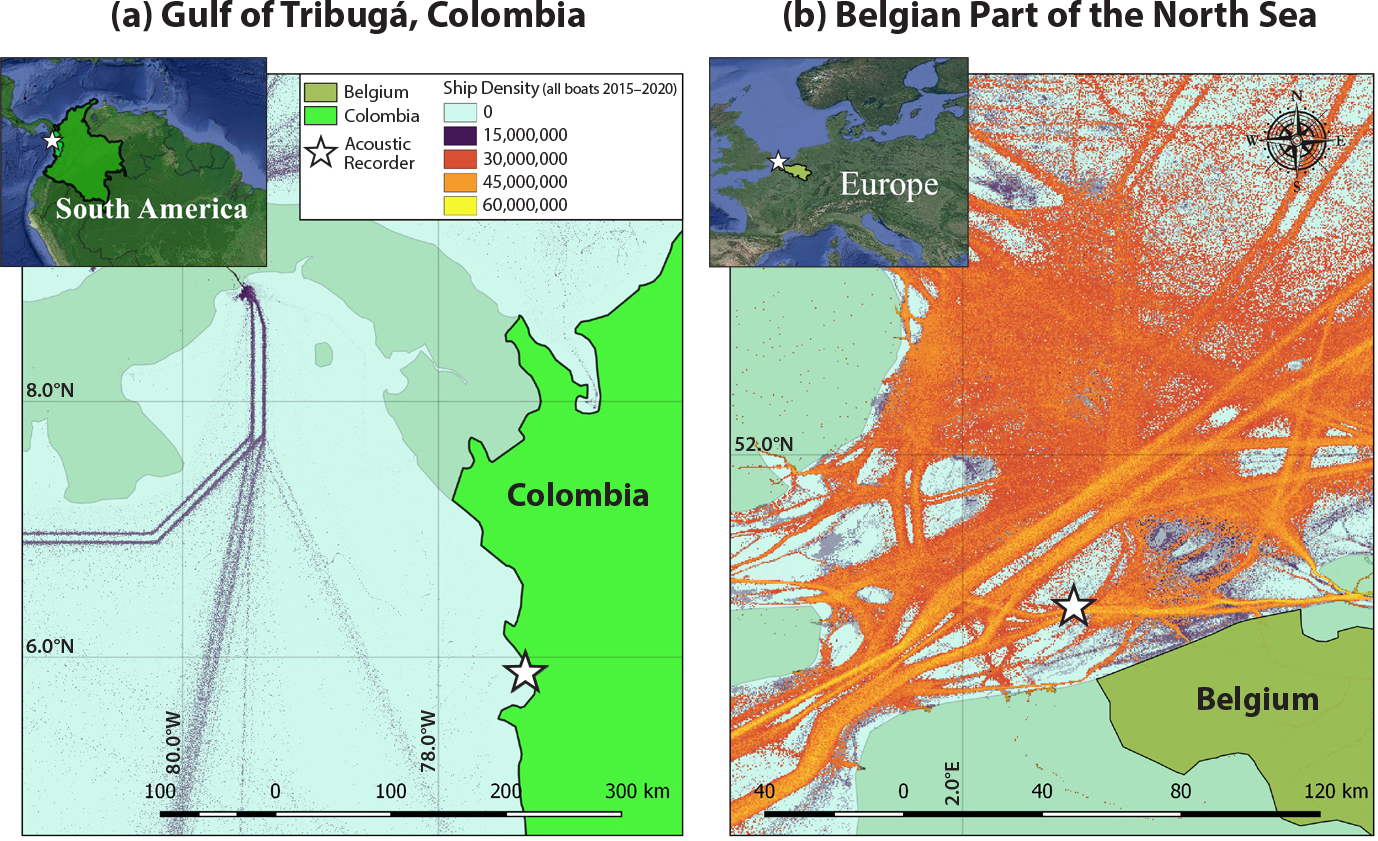
Here, we describe two study regions with vastly different soundscapes, characterized by extremely different shipping densities (Figure 2). The first study region, the Gulf of Tribugá, Colombia, is “less disturbed” by undersea noise (closest to pristine). It serves as a general marine soundscape baseline for comparison with possible future disturbances from port construction and operation. By contrast, the second study region, the Belgian part of the North Sea (BPNS) is located in a “more disturbed” area of very exploited shallow waters. Its baseline is being used to monitor the effects of noise reduction policies. We chose October 16, 2020, at 12:00 until October 17, 2020, at 07:30 (local time) as the day for our soundscape comparison. Our hypothesis is that biophony dominates the Gulf of Tribugá while anthropophony dominates the BPNS.
|
|
Gulf of Tribugá
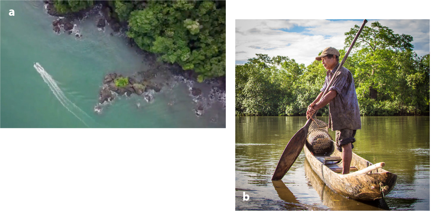
The main goals of the PHySIColombia Project were to identify which sound sources exist in the Gulf of Tribugá (Figures 2a and 3); to measure the contributions of sounds from small boats, humpback whales, fish, dolphins, and storms/tides; and to establish the cycles for each source (Rey-Baquero et al., 2021). One of the rainiest areas on Earth, Tribugá boasts high biological diversity. Due to its high ecological value, it is a newly designated Hope Spot (an ecologically unique area of the ocean designated for protection). This area currently contains no shipping lanes, so boat noise is generated only from small-scale ecotourism and artisanal fishing. It is part of the breeding grounds for humpback whale (Megaptera novaeangliae) Stock G, a species whose survival relies on acoustic communication. The longest monitored deployment site (from 2018 to 2021) is Morro Mico (5°52'10.1''N, 77°18'40.7''W), in the north of the Gulf just south of Utría National Park, about 0.5 km from the coast. Data were collected at 25 m depth using an ecological acoustic recorder (Oceanwide Science Institute) programmed to record for 10 minutes every half hour at 15.625 kHz sampling rate.
|
|
Belgian Part of the North Sea
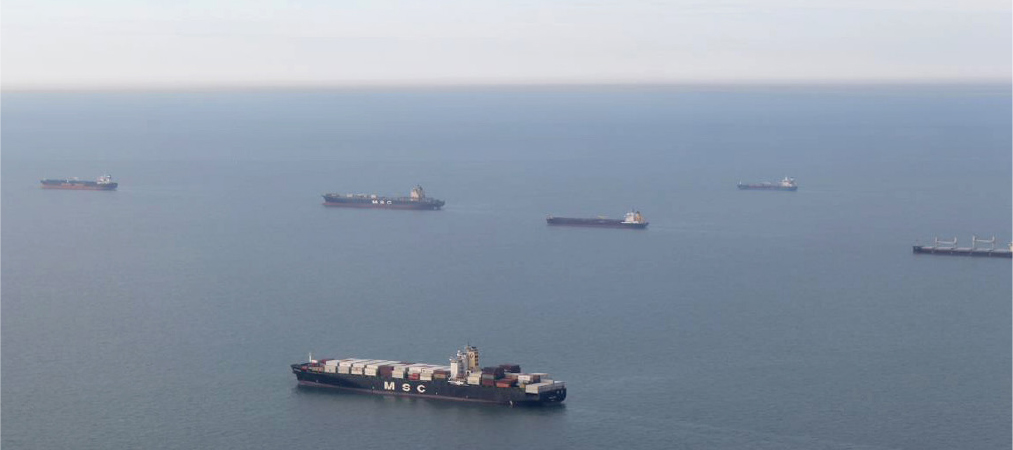
As a part of the Belgian LifeWatch project, an acoustic network was deployed that records continuously in different locations of the BPNS, one of the busiest ocean areas in the world. This shallow sea is characterized by sand banks and a wide variety of sediment that hosts five benthic communities.
The aim of this network is to measure underwater sound across benthic habitats. The lack of historical data prohibits defining an unimpacted soundscape baseline. The location for the site used to compare with the Gulf of Tribugá is the Westhinder shipwreck (51°22'52.2''N, 2°27'9.72''E; Figures 2b and 4), which is next to an anchor zone for commercial ships and close to a shipping lane. Therefore, shipping and other anthropophony constitute an overwhelmingly dominant ocean sound source. It is also populated with harbor porpoises (Phocoena phocoena), but their echolocation frequency is too high for the recorder used, so they cannot be seen in the acquired data. Data were collected with a SoundTrap 300 HF (Ocean Instruments) attached to a tripod at 1 m above the sea bottom at 96 kHz sampling rate, recording continuously. It was 32 m deep and about 30 km from the coastline.
|
|
Spectrogram Visualization
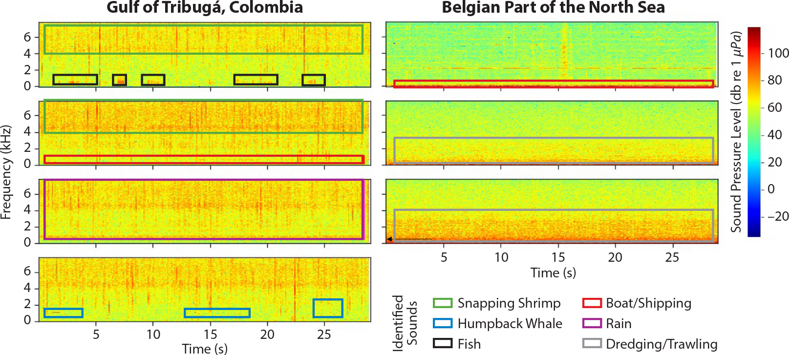
We identified different sounds using spectrograms generated by Raven Pro 1.6 software (Figure 5). Marking the spectrograms manually when each sound type occurred allowed us to determine the schedules on which animals, natural events, and human-made noises operated. The largest contribution to the Gulf Tribugá soundscape was from singing humpback whales, then shrimp, and finally fish. Anthropophony was primarily from small boats, but occasionally from one or two larger shrimping boats. The loudest geophony sounds came from rain and wind, while the sloshing of the tide and crashing of waves onshore commonly existed in the background.
In contrast, anthropogenic noise dominates the BPNS soundscape. The identified sounds were generated by large ships, probably commercial or fishing. Another identified sound is possibly dredging or trawling, which is concentrated at about 1 kHz or below and is constant and prolonged.
|
|
Spectral Probability Density Comparison
To compare the soundscapes of both locations, we computed the spectral probability density (SPD) of each location using pypam (https://github.com/lifewatch/pypam). SPD is useful for computing the statistical distribution of underwater noise levels across the frequency spectrum (Merchant et al., 2013). To compute the SPDs, the audio files were divided into one-minute samples. Frequency distribution and the probability of each frequency appearing at a certain sound level (from 20 to 140 dB re 1 μPa) were computed, and both sites were processed to remove the direct current (DC) electrical noise generated by the instruments. The data from the BPNS location were downsampled to match the sampling rate used in Tribugá so that the frequency and time resolution of both SPD computations would match.
The 1st, 10th, 50th, 90th, and 99th percentiles of the SPD represent the intensities and contributions of sounds in the soundscape. The 1st percentile represents sounds that occur 99% of the time but are low intensity, and the 99th percentile represents the loudest sounds, which occur only 1% of the time. Depending on the soundscape, each percentile can represent different sound sources.
Biophony dominates Tribugá’s soundscape: the 1st percentile represents the sounds of snapping shrimp (sound energy above 4,000 Hz); the humpback song is represented by the 10th and 50th percentiles, especially if there are several whales singing at once. One common high-energy frequency band in song (~300 Hz) is visible as a less evident peak (when there are fewer singers) in the 90th percentile. Another peak above 1,000 Hz could represent another band in humpback whale song, but because it is only in the 90th percentile for this day, it likely is due to rain (Figure 6). The 99th percentile has a predominant peak around 300 Hz, and there are several other peaks between 50 Hz and 1,000 Hz that represent bands of noise from small whale-watching and fishing boats that speed by Morro Mico quickly.
|
|
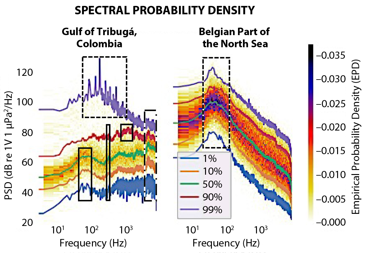
In the BPNS’s SPD, there is a clear peak between 20 Hz and 300 Hz, which is known to be the frequency band for shipping noise. Compared to Tribugá, ship noise is present for longer durations in the BPNS. Biophony present in the BPNS is mostly masked by anthropophony, and the contribution of marine animals to the soundscape in the BPNS is less frequent than anthropophony, so it is not obviously represented in the SPD. In addition, recorded sound levels are generally louder in the BPNS than in Tribugá (Figure 6). The loudest sounds in the BPNS are lower in frequency, while in Tribugá the higher frequencies are louder. Because sound sources are more infrequent in Tribugá (i.e., no shipping lane exists to create a constant band of noise), it has greater variability in frequency and loudness, which correlates with some studies that link biological sounds to greater variation of sounds in frequency and time (Wilford et al., 2021).
Conclusions and Perspectives
By first establishing acoustic baselines in less and more noisy ocean regions, monitoring soundscapes over time can be a cost-effective method for assessing the health of marine ecosystems. Some scientists are developing acoustic indices that would link acoustic features to biodiversity or other biological indicators (Wilford et al., 2021). Few standards exist for sensor deployment configuration, making ecosystem comparisons challenging or not feasible, and no global acoustic indicator yet exists. However, various groups are working to standardize marine acoustic data acquisition and to develop a more general approach to establishing different ecosystems’ soundscapes. How long or how often the recorder is active also influences data analysis, so it is often not possible to compare different time periods. Because many studies focus on a single region and have budget constraints, data often come from one type of environment and deployment configuration. Several recorders spaced at intervals could capture soundscapes in a single area with varying seafloor topography or differing sediment types.
Biophony dominated the Gulf of Tribugá, while anthropophony dominated the BPNS and masked any biophony. Our analysis demonstrated that different sources drove each soundscape. If the sound sources are known, SPD can be interpreted by specialists to describe the soundscape, but unknown sources remain a limitation for soundscape studies.