Two saildrones participated in the Salinity Processes in the Upper-ocean Regional Study 2 (SPURS-2) field campaign at 10°N, 125°W, as part of their more than six-month Tropical Pacific Observing System (TPOS)-2020 pilot study in the eastern tropical Pacific. The two saildrones were launched from San Francisco, California, on September 1, 2017, and arrived at the SPURS-2 region on October 15, one week before R/V Revelle. Upon arrival at the SPURS-2 site, they each began a two-week repeat pattern, sailing around the program’s central moored surface buoy. The heavily instrumented Woods Hole Oceanographic Institution (WHOI) SPURS-2 buoy serves as a benchmark for validating the saildrone measurements for air-sea fluxes. The data collected by the WHOI buoy and the saildrones were found to be in reasonably good agreement. Although of short duration, these ship-saildrone-buoy comparisons are encouraging as they provide enhanced understanding of measurements by various platforms in a rapidly changing subsynoptic weather system. The saildrones were generally able to navigate the challenging Intertropical Convergence Zone, where winds are low and currents can be strong, demonstrating that the saildrone is an effective platform for observing a wide range of oceanographic variables important to air-sea interaction studies.

 

Saildrone SD1006 starting its journey from San Francisco, California, to the SPURS-2 region in the eastern tropical Pacific. > High res figure

Introduction

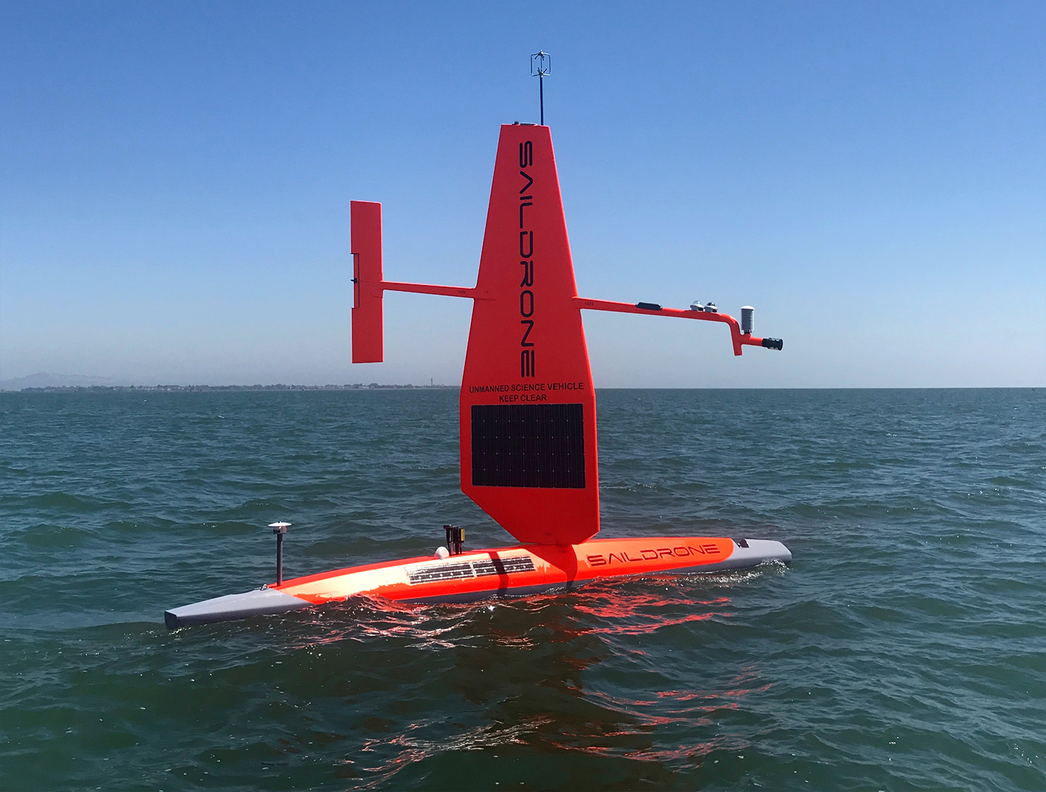
With the ability to transit thousands of kilometers while making surface observations similar to a moored buoy, the saildrone unmanned surface vehicle (USV), manufactured and piloted by Saildrone Inc., could contribute in important ways to the Global Ocean Observing System (GOOS). Saildrones are powered by renewable energy, using wind for propulsion and solar energy for vehicle control, sensor operation, onboard data processing, and real-time data telemetry. Through a Cooperative Research and Development Agreement (CRADA) between NOAA’s Pacific Marine Environmental Laboratory (PMEL) and Saildrone Inc., sensors for measuring 22 essential ocean and climate variables (EOVs and ECVs) and high-​frequency platform motion were integrated into the saildrone system (Cokelet et al., 2015; Meinig et al., 2015, in press; Zhang et al., 2017), making the saildrone sensor suite almost as complete as that of a Tropical Atmosphere Ocean (TAO) buoy (McPhaden et al., 1998; Figure 1). While the ability to navigate enables a saildrone to make repeat cross sections and do adaptive sampling and surveys, the motion of the platform can cause noise in the observations, requiring careful measurement of platform motion to correct measured variables.

 

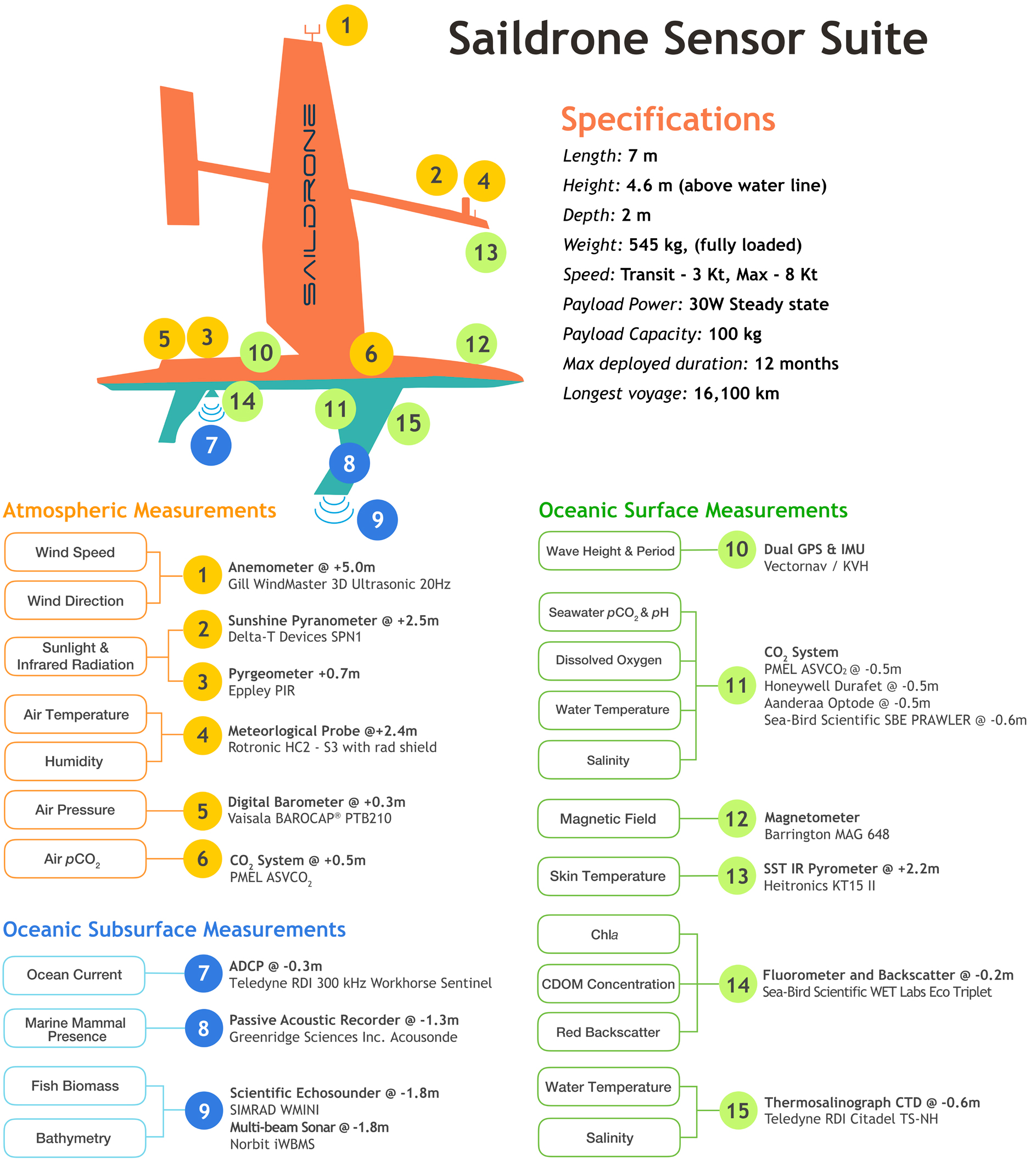
Figure 1. Saildrone diagram showing all the sensors and measurement locations for 22 essential ocean and climate variables. Exact instrument placement may vary by mission. Adapted from Zhang et al. (2017). > High res figure

 

For the Tropical Pacific Observing System (TPOS)-2020 (Cravatte et al., 2016) pilot study, two saildrones were launched from San Francisco, California, on September 1, 2017. A main goal of this mission was to evaluate the feasibility of using saildrones for observing tropical air-sea interaction. The vehicles transited to the equator at ~125°W via the Salinity Processes in the Upper-ocean Regional Study 2 (SPURS-2) site at 10°N, 125°W, moved further south to the TPOS area, and returned to California in May 2018 (Figure 2). In addition to testing the navigation of saildrones in the low-wind and strong-current conditions of the tropical Pacific, challenging to any sailing vessel, one main objective was to compare the air-sea interaction processes at SPURS-2 measured by the saildrone to those measured by the program’s central buoy (Farrar and Plueddemann, 2019, in this issue). The heavily instrumented central buoy at 10°N, 125°W, deployed by Woods Hole Oceanographic Institution (WHOI), provided known standards for comparison with the saildrone. There was also a six- to seven-​hour time period when R/V Revelle was in close proximity to both the saildrones and the WHOI buoy, so measurements from all participating platforms can be compared.

 

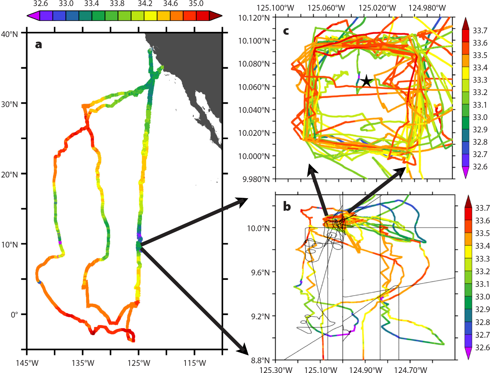
Figure 2. (a) Saildrone tracks of Tropical Pacific Observing System Mission (2017–2018) colored by sea surface salinity (SSS). (b) Zoom-in of SPURS-2 intense observation area showing saildrone tracks with SSS in color and Revelle tracks as black lines, during October 17–November 16, 2017. (c) Zoom-in of the saildrone tracks around the central SPURS-2 buoy with saildrone SSS in color and buoy location indicated by a star, October 18–November 6, 2017. Note different color scales in (a), (b), and (c). > High res figure

 

This paper presents: (1) measurements for air-sea heat fluxes critical for SPURS-2 to better understand upper-ocean stratification beneath the Intertropical Convergence Zone (ITCZ) in the Eastern Pacific Warm Pool, and (2) comparisons of traditional measurement methods with new USV technology.

 

Saildrone Measurements

Saildrone Mission in SPURS-2

The two saildrones (SD1005 and SD1006) arrived at the SPURS-2 field observation region one week before R/V Revelle. On October 18, 2017, the drones began to collect observations along the four 10 km sides of a box around the anchor location of the WHOI buoy (Figure 2c), maintaining a 4.3 km radius watch circle around the buoy. The two saildrones stayed on opposite sides of the buoy as they sailed around it anticlockwise. As planned, it took about 1.5 days for each saildrone to complete the box, so that observations from the two saildrones could resolve inertial oscillations, which have a period of about three days in the SPURS-2 region. This was partially successful, although conditions became difficult for navigation at times.

On October 19, the saildrone acoustic Doppler current profilers (ADCPs) measured surface currents up to 0.9 m s^–1 (not shown), while the winds were calm with speeds as weak as 0.2 m s^–1. The two saildrones could not overcome the currents and drifted eastward (Figure 2b). They returned to position on October 21 and successfully maintained their tracks around the buoy during the rest of the intercomparison period. On October 23 and 27, they sailed away to allow space for Revelle to service the buoy. They also sailed next to Revelle to enable comparison of the saildrone sensors with shipboard instruments on November 1. After the buoy was recovered, the two saildrones completed two back-and-forth meridional sections along 124.8°W and 125.2°W between 9°N and 10°N against mostly southerly wind. Between 9°N and 9.25°N, the saildrones again encountered low winds (<0.5 m s^–1) and drifted eastward before returning to the meridional sections. Close communication between the captain and chief scientist aboard Revelle and the scientists and saildrone pilots on shore was key to the success of the saildrone participation in the SPURS-2 field campaign and to intercomparisons of their measurements with those of other platforms.

 

Saildrone-Measured Variables for Air-Sea Fluxes

Variables validated here are key “state variables” that are routinely used to derive air-sea surface heat fluxes and momentum flux using bulk algorithms (Fairall et al., 2003; Edson et al., 2013). Measurements of these variables at sea are challenging. The radiometers that measure downwelling shortwave (SW) and longwave (LW) radiation are designed to sense the hemisphere above them and are intended to stay level when taking measurements. Instruments installed on ocean observing platforms, however, can rarely be leveled due to the influence of waves, currents, and winds. Figure 3 shows the probability density function (PDF) of the pitch and roll of the saildrone mast and spar (which serve, like an airplane wing, to provide thrust), where the meteorological sensors are mounted (Figure 1 and saildrone picture). Accurate measurements of high-frequency platform motion are therefore essential for motion correction of measured variables, especially for SW radiation and wind that are sensitive to tilts. Additionally, strong vertical gradients are present in air temperature (T_air), relative humidity (RH), and wind near the air-sea interface, with logarithmic profiles dependent upon height and stability. These logarithmic profiles need to be estimated using the bulk flux parameterization (Fairall et al., 2003; Edson et al., 2013) to adjust these measurements to a standard height, taking into account height changes in the saildrone sensors due to tilts.

 

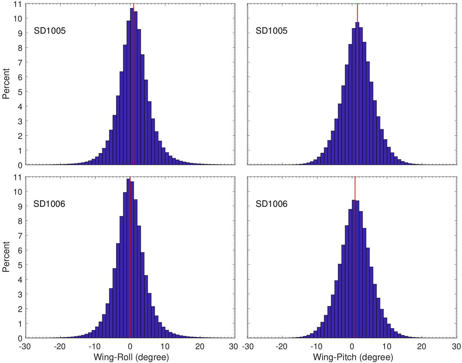
Figure 3. Histograms of the 10 Hz pitch and roll angles of the saildrone wing, showing distribution of tilts of every 1° bin in percentage. Saildrone SD1005 and SD1006 exhibit mean roll of 0.94° and −0.11°, with standard deviations (std) of 4.76° and 4.64°, respectively, mean pitch of 1.53° and 0.85°, with std of 4.64° and 4.67°, respectively. > High res figure

 

Compared to other USVs that do not have superstructures, the saildrone wing and boom allow sensors to be mounted at 3–6 m above the ocean surface. This places them above the wave boundary layer for most conditions, which provides an important advantage for air-sea interaction observations. The saildrone sensor heights are comparable to or higher than instruments on widely used air-sea flux Reference Site buoys (Colbo and Weller, 2009; Send et al., 2010; Cronin et al., 2015). However, mounting locations for saildrone sensors have some limits. Ideally, all sensors need to be placed in unobstructed air flow and space clear of shade and reflection of radiation. For surface buoys, most sensors are mounted at the top of buoy tower for best clearance, though flow distortion often occurs around crowded sensors. For saildrones, sensor placement must also consider optimizing the balance and control of the saildrone wing. The current saildrone configuration (Figure 1 and saildrone picture) has the wind sensor placed at the top and out into the air as much as possible to minimize flow distortion, but has to leave the SW radiation sensor on the boom and the LW sensor placed on the hull, away from the wing as much as possible for better clearance. The air temperature and humidity sensor (with Teflon shield) is also sensitive to air flow because of a self-heating effect in low wind conditions. While any structure next to the sensor can potentially slow down air flow, placement in front of the wing allows air flow from the wind and the saildrone speed to blow into the sensor from the two front quadrants (as illustrated in the saildrone picture with the saildrone sailing to the right).

Measurement of wind is sensitive to platform motion and orientation, and therefore the three-dimensional ultrasonic-anemometer (Gill WindMaster) was set to measure three-dimensional wind velocity (u, v, w) at 10 Hz, in sync with the combined GPS inertial navigation system (INS) and inertial measurement units (IMUs) that measured the three-axis motion of the vehicle’s hull and wing and the saildrone’s speed over ground (SOG). High-frequency motion corrections were completed on board in real time, resulting in u, v, and w relative to the fixed Earth, in Earth coordinates. One-minute averaged (u, v, w) data were telemetered to shore, while high-frequency (10 Hz) data were stored on board for later download when the saildrones returned to port at the end of the mission. Wind speed was then calculated from u and v. The 10 Hz IMU data are also used to determine the tilt of the wing and therefore the instant measurement heights of wind, air temperature, and humidity.

The SW measurement comprises total insolation from the sun and the diffuse component of scattered sunlight from the sky, from which the direct component can be computed. Due to the tilt of the moving platform from the horizontal plane, changes in the angular orientation of direct solar radiation to the instrument can introduce significant offsets to the measured SW radiation (e.g., Long et al., 2010). Based on the high-frequency roll, pitch, and heading angles from the wing IMUs, we were able to estimate the true solar zenith angle with respect to the moving platform (i.e., angle of the location of the sun in the SPN1 field-of-view and the normal to the tilted platform). The SPN1 Sunshine Pyranometer (Delta-T Device, UK) measures both direct and diffuse solar irradiance at a fast sampling rate of 5 Hz, allowing for a tilt correction to be applied to the direct SW radiation following Long et al. (2010). The diffuse component was assumed to be nearly isotropic and thus not overly affected by moderate tilt of the platform. Within ±10° tilt from the horizon, the tilt-corrected SW radiation was found to fall within the range of the manufacturer accuracy of SPN1 (Long et al., 2010). We further limited the tilt-corrected SW data to solar zenith angle lower than 80^o, in consideration of the cosine response in direct SW measurements from SPN1 (Badosa et al., 2014).

All other meteorological variables were sampled at 1 Hz, with one-minute averages telemetered in real time. The primary CTD for sea surface temperature (SST) and sea surface salinity (SSS) is the Teledyne Citadel TS-NH Thermosalinograph at 0.6 m depth. A pumped Sea-Bird Scientific (SBE) CTD that was integrated into the PMEL Autonomous Surface Vehicle CO₂ (ASVCO₂) system, which is based on the moored pCO₂ system described by Sutton et al. (2014), also measured SSS and SST at 0.6 m but at a slower rate, every 30 minutes to one hour. The Citadel CTD was installed on the saildrone with three-dimensional printed inlet and exit ports, which plumbed the sensor into the flow-through tube within the keel. These custom ports affected the calibration of the inductive sensor, resulting in a constant offset of 0.4 PSU in salinity measurements, determined by comparing it to the SBE CTD. Salinity records from the Citadel are therefore adjusted to match the SBE CTD during pre-​mission calibration and the first 20 days of the TPOS Mission.

 

Validating Saildrone-Measured Variables

Saildrone-Buoy Comparison

Here, we compare eight variables measured by the saildrone air-sea flux suite and the WHOI buoy’s Air-Sea Interaction METeorology System (ASIMET), which has a long history of deployment and well-documented accuracy (Colbo and Weller, 2009). These variables are downwelling SW radiation and LW radiation, T_air and RH, wind speed, wind direction, SST, and SSS. Buoy wind (measured at 3.23 m), T_air (2.89 m), and RH (2.89 m) are adjusted to saildrone sensor nominal heights at 5.0 m, 2.4 m, and 2.4 m respectively, using the COARE 3.5 bulk algorithm (Fairall et al., 2003; Edson et al., 2013). Similarly, the instantaneous measurement heights of saildrone sensors due to tilt, determined by high-frequency (10 Hz) measurements of pitch/roll of the saildrone wing, are also adjusted to the nominal heights using COARE3.5. The bulk SST and SSS measured by saildrone at 0.6 m depth (Citadel CTD) are compared to the SST and SSS measured at 0.95 m by the WHOI buoy, as well as by the pumped SBE CTD on the saildrone.

Figure 4 shows a time series of WHOI ASIMET variables (black) and saildrone measured variables (red) when the saildrones were within 12 km of the buoy (a distance chosen to ensure all measurements along the boxes in Figure 2c are included). Figure 5 shows scatter plots of saildrone and ASIMET measurements. Measuring these state variables for air-sea flux quantification is challenging at sea, with limiting factors such as platform tilt and sea spray affecting both buoy and saildrone. In comparisons with nearby research ship measurements and redundant sensors on the same buoy, ASIMET measurement errors (including both instrument and field errors) are thoroughly documented in Colbo and Weller (2009) and Bigorre et al. (2013). The SPURS-2 WHOI buoy’s ASIMET thus provides a benchmark comparison for saildrone measurements.

 

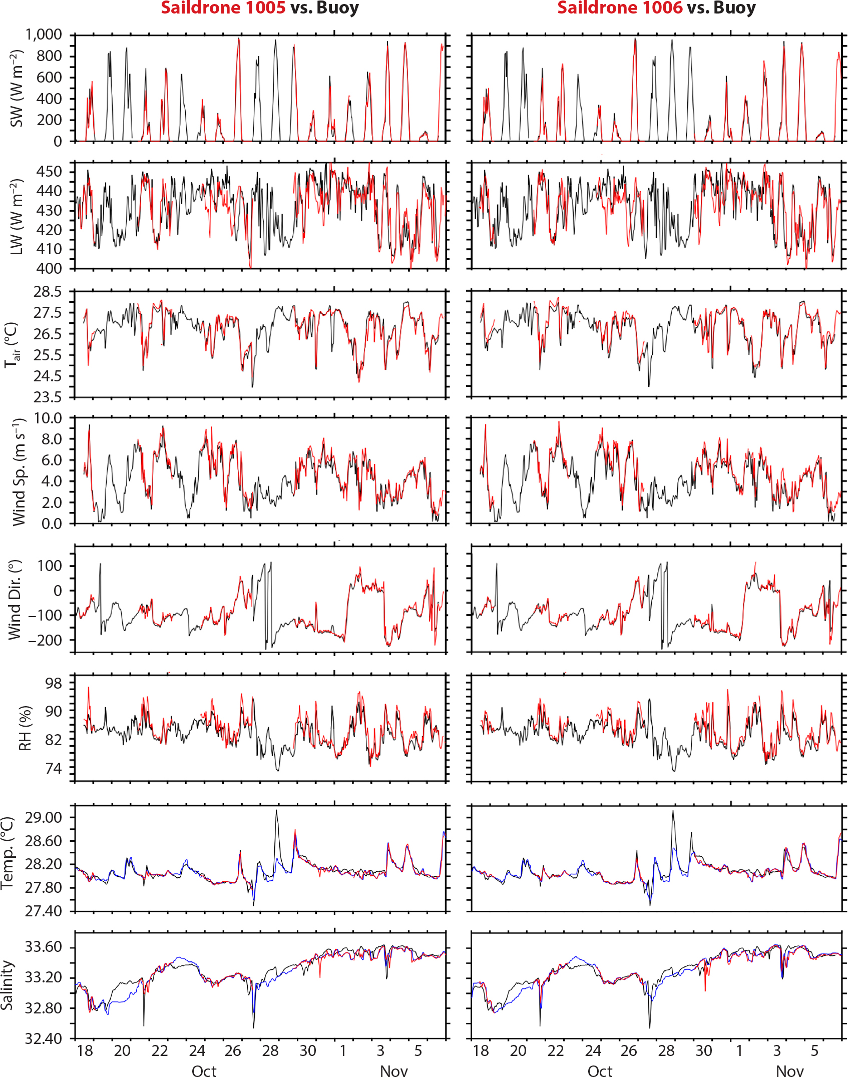
Figure 4. Saildrones (red) versus Woods Hole Oceanographic Institution (WHOI) Air-Sea Interaction METeorology System (ASIMET) measurements (black) for downwelling shortwave (SW) and longwave (LW) radiation, air temperature (Tair), wind speed and direction, relative humidity (RH), sea surface temperature (SST), and sea surface salinity (SSS). Blue lines are SST and SSS measured by the saildrone ASVCO2 SBE CTD. Tair/RH of both buoy and saildrones were adjusted to 2.4 m, wind adjusted to 5 m (see text). Buoy SST/SSS measurements (black) were at 0.95 m, saildrone (red = Citadel; blue = SBE) at 0.6 m. > High res figure

 

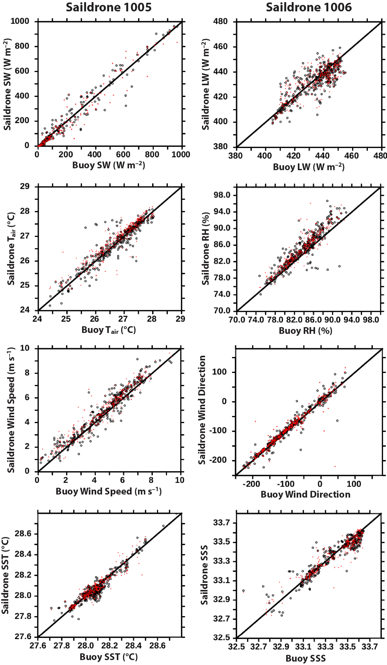
Figure 5. Scatter plots of saildrone versus WHOI ASIMET measurements. Black circles: SD1005 vs. ASIMET; Red dots: SD1006 vs. ASIMET. The 1:1 line is shown for comparison. Regressions are in Table 1. > High res figure

 

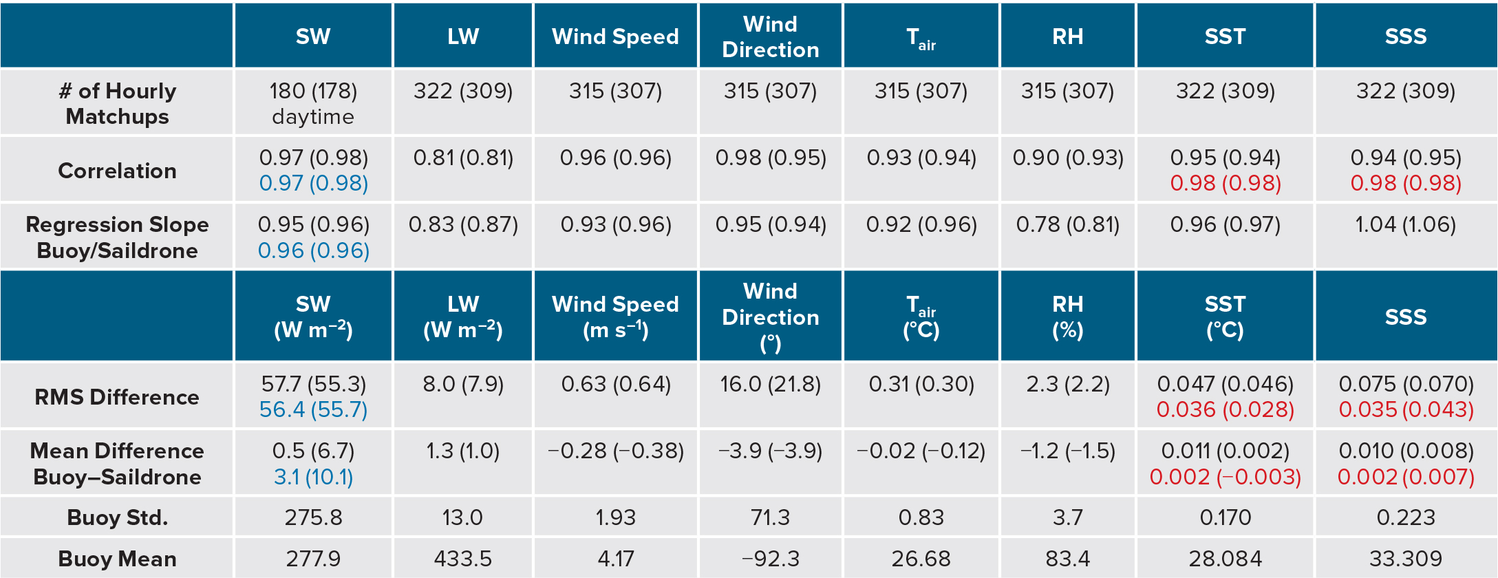
The ASIMET SW radiation sensor is the Eppley precision spectral pyranometer (PSP). Here, the total SW radiation by Delta-t SPN1 is compared to the Eppley PSP measurements. The Eppley PSP is considered a more reliable sensor, with manufacturer specified accuracy of ±2% (5 W m^–2), but its response timescale is about 5 s. The SPN1 on the other hand has a response time of 0.1s, but manufacturer specified uncertainty of ±5% (10 W m^–2). Due to saildrone’s high-frequency platform motion and high degree of tilt, we chose the fast response SPN1 and rely on the ratio of direct and diffuse irradiance and high-frequency IMU pitch/roll/heading to derive the corrected total SW radiation following Long et al. (2010). To reduce the uncertainty of SPN1s, we set up an on-land calibration test to compare SPN1s with the Eppley PSPs, as recommended by Badosa et al. (2014). Of the four SPN1s ordered for the TPOS mission, we found three to be within 2% agreement with Eppley; the manufacturer agreed to replace the outlier with a new sensor. Given that both buoy and saildrones are subject to tilt and that each instrument has specified errors, the good agreement of SW radiation measured by the two platforms is a pleasant surprise. Their mean differences (0.5 and 6.7 W m^–2, Table 1) are within or close to the ASIMET daily measurement uncertainties (6 W m^–2). The reduction of uncertainty is likely due to the large number of hourly matchups (Table 1) involved in the averaging. The RMS differences between the two saildrones’ measurements and the ASIMET are 57.7 W m^–2 and 55.3 W m^–2, respectively, larger than the instantaneous measurement error of ASIMET (>20 W m^–2) but not much larger than the uncertainty range (>40 W m^–2), assuming both platforms have the same magnitude of instant error (Colbo and Weller, 2009). The saildrones were separated from the buoy by up to 12 km; natural spatial variability due to broken clouds may have also contributed to the large RMS differences. Note that the mean (275.8 W m^–2) and standard deviation (std) (277.9 W m^–2) of downwelling SW radiation measured by ASIMET, a measure of SW radiation variability at the SPURS-2 site (or signal to be resolved by the measurements), are much larger than the RMS differences. It is also encouraging to see the very high correlation (0.97 and 0.98) of the saildrone and ASIMET SW measurements (Table 1, Figures 4 and 5), with slopes close to 1 (0.95 and 0.96). There may be a question about whether the high correlation is due to the large diurnal signals of SW radiation in the data. The comparison of daily mean (not shown), though reduced to only eight daily data points, also shows high correlation (0.99 and 0.99) and slopes close to 1 (0.97 and 0.96). Table 1 shows comparisons of uncorrected SW saildrone radiation to buoy data (blue values in Table 1). Though the tilt correction did reduce the mean difference between saildrone and buoy measurements, it had no impact on the RMS differences or the correlations. Although the improvement from tilt correction on the mean differences is small (2–4 W m^–2), the instantaneous differences between the corrected and uncorrected data can sometimes reach ±70–100 W m^–2. During this first TPOS mission, the SPN1s were installed pitch-down as an attempt to compensate for a potential upward offset observed during saildrone tests off California. However, the upward offsets in the tropical Pacific were only 1°–2° (mean pitch in Figure 3), smaller than anticipated and resulting in a mean tilt of about 5° from the horizon. Although effects of this tilt are corrected in the tilt correction (Long et al., 2010), the SPN1s will be mounted more horizontally in future missions.

 

Table 1. Comparison of SD1005 (SD1006) with WHOI ASIMET data when saildrones were within 12 km of the central buoy location. Wind, air temperature (Tair), and relative humidity (RH) at buoy and saildrone measurement heights were adjusted to saildrone sensor nominal heights at 5 m and 2.4 m (see text). Saildrone and buoy sea surface temperature (SST) and sea surface salinity (SSS) were measured at 0.6 m and 0.95 m, respectively. A constant offset of 0.4 psu was applied to saildrone Citadel salinity (see text). Correlations and differences between saildrone Citadel and Sea-Bird CTD data during SPURS-2 are shown in red. Comparisons of raw saildrone shortwave radiation without tilt correction and buoy measurements are shown in blue. Matchups of hourly shortwave radiation count only daytime hours. SW = Shortwave radiation. LW = Longwave radiation. > High res table

 

Both the saildrone and the ASIMET employ the Eppley precision infrared radiometer (PIR) as the LW radiation measurement sensor. The manufacturer specified uncertainty for the PIR is 5 W m^–2. The tilt of the platform has less impact on LW than on SW radiation measurements, but LW radiation is challenging to measure. The Eppley PIR LW radiation is calculated from measured thermopile voltage and dome and case temperatures, which are affected by the module’s electronic stability, solar contamination, thermal gradients in the dome and case temperatures, and dome contamination at sea. The carefully analyzed total daily and annual mean uncertainty of LW radiation by ASIMET is 4 W m^–2 with instantaneous errors of 7.5 W m^–2 (Colbo and Weller, 2009). The mean difference between the two saildrone measurements and ASIMET (1.3 W m^–2 and 1.0 W m^–2) are well within the ASIMET mean uncertainty. The RMS differences are comparable to the instantaneous error of ASIMET-measured LW radiation. The correlation between saildrone and ASIMET LW radiation is 0.81 for each drone, well above 95% significance level (Table 1, Figures 4 and 5). The regression slopes are 0.83 and 0.87, respectively. The correlations of LW radiation measured by saildrone and buoy are the lowest among the compared variables. This is likely due to the relatively small signal of LW variability under the ITCZ, with a std of 13 W m^–2 and a mean LW radiation of 433.5 W m^–2.

For T_air and RH, both saildrone and ASIMET use Rotronic products, with Rotronic HC2-S3 on Saildrone and Rotronic MP101A on ASIMET. Analysis by Colbo and Weller (2009) suggests that the total uncertainty of ASIMET T_air and RH are 0.1°C (more in low winds <3 m s^–1) and 1% RH (3% RH in low winds), respectively. Their instantaneous errors are 0.2°C (more in low winds) and 1% RH (3% RH in low winds). The mean and RMS differences between the saildrone and ASIMET measurements (Table 1) are within the mean and instantaneous errors of ASIMET T_air and RH, and their correlations are all above 0.9 (Table 1, Figures 4 and 5). The regression of saildrone T_air to ASIMET T_air is 0.92 (0.96), while the regression of saildrone RH is much lower, 0.78 (0.81). There is a tendency for larger differences when the humidity is higher (Figure 5). The calibration in the humidity chamber does show a higher bias of both sensors at higher humidity. However, since the bias is within 1% (the error specified by the manufacturer) and the latent heat fluxes are small at high humidity values, no adjustment is applied to these measurements.

ASIMET’s wind sensor is the propeller and vane R.M. Young Wind Monitor, with a total mean observational error of 1% or 0.1 m s^–1 (whichever is larger) and instantaneous error of 1.5% or 0.1 m s^–1, according to Colbo and Weller (2009). This sensor’s uncertainties are larger in low winds due to the bearing drag of the propeller and vane system. The saildrone wind speeds are highly correlated with the ASIMET winds, with a correlation of 0.96 for both saildrones and regressions of 0.93 and 0.96. But the saildrone measured wind speeds are 0.28 m s^–1 and 0.38 m s^–1 higher than ASIMET winds, and their RMS differences are 0.63 m s^–1 and 0.64 m s^–1, respectively. Although the mean differences (~0.3 m s^–1) are small, they are higher than the 0.1 m s^–1 observational error of subtropical buoys (Colbo and Weller, 2009) but within the characterized observation error ±0.3 m s^–1 (3%) of R.M. Young wind sensors on TAO buoys in the tropical Pacific (Cronin et al., 2006). Flow distortion around the buoy structure is believed to cause a wind speed bias ranging from −1% to +3.5%, depending on the angle of the wind to the buoy’s wind vane (Emond et al., 2012; Bigorre et al., 2013). Flow distortion around the saildrone may also introduce bias, though analysis of three-​dimensional, high-frequency wind data suggests it may be smaller than around heavily instrumented buoys (Douglas Vandemark and Marc Emond, University of New Hampshire, pers. comm., 2017).

 

“One of the primary goals of the pilot study discussed here was to evaluate the saildrone as a potential platform for the Tropical Pacific Observing System to monitor surface air-sea interaction and biogeochemistry in a variety of sampling modes.”

 

Saildrone wind direction measurements compare reasonably well with ASIMET measurements, with correlation of 0.96 (0.96) and regression of 0.93 (0.96). The instant error of ASIMET R.M. Young wind direction is 6° (more in low winds), and the mean error is 5° (Colbo and Weller, 2009). The mean difference between saildrone and buoy measurements (3.9°) is within the mean error of ASIMET. The RMS differences (16.0° and 21.8°) in wind direction are higher than the target value of 12° (twice the ASIMET instant error) that we would like them to be. But they are much smaller than the local variability (71.3°, std of wind direction in Table 1), suggesting that the saildrone measurements are adequate to resolve wind direction changes in the SPURS-2 region.

Two CTDs on board the saildrones measure SST and SSS at 0.6 m. The Citadel TS-NH sampling rate is set at 1 Hz, with a burst of 12 measurements each minute to get one-minute data. The SBE CTD sampling scheme is every 30 minutes to one hour, synced with the ASVCO₂ measurements. Because of the high-frequency measurements, the Citadel TS-NH is the saildrone’s primary CTD, but the SBE CTD is pumped with anti-foulant to prevent salinity drift. The SST measurements of the ASIMET are also from an SBE CTD but at 0.95 m depth. The SST observations are highly precise: the mean differences between the Citadel SST and the WHOI surface CTD are 0.011° and 0.002°C, their RMS differences are 0.047° and 0.046°C, and their correlations are 0.95 and 0.94. Not surprisingly, the co-located Citadel TS-NH and SBE CTD on the saildrones exhibit even better agreement (Table 1).

SSS measurements are very challenging over long durations at sea, mainly due to biofouling. The initial comparison reveals a large fresh bias in ASIMET SSS of more than 0.3. Further investigation by comparing the ASIMET SSS with deeper salinity records of the WHOI buoy suggest a significant drift of SSS starting in May 2017 after nine months of deployment. As an independent calibration, the Revelle shipboard CTD cast, collected on October 23, 2017, when the ship was servicing the buoy, is used to correct the SSS drift of the WHOI sensor with a linear fit between May 6 and October 23. The resulting mean differences between Citadel and ASIMET corrected SSS are 0.010 and 0.008, within Citadel’s specified instrument accuracy for salinity measurements (± 0.015). They have very high correlations (>0.94) and close-to-1 regressions, with RMS differences of 0.075 and 0.070, respectively. The saildrones’ co-located Citadel and SBE CTDs are in even better agreement (Table 1).

 

Ship-Saildrone-Buoy Comparison

Among measurements by the various platforms, shipboard measurements generally have the highest quality because sensors can be regularly attended, adjusted, and cleaned, as needed. However, due to the demanding schedule of each science cruise, the opportunity for the research vessel to be on station with other platforms was rare. During SPURS-2, Revelle designated six hours for ship-saildrone-buoy comparisons (Figure 6). Shipboard data were kindly provided by Jim Edson of WHOI, with T_air, RH, and wind speed all adjusted to 10 m height. Saildrone and buoy data were accordingly adjusted to 10 m using the COARE3.5 bulk algorithm. Due to the short duration, 10-minute averages are compared rather than the hourly averages in saildrone-​buoy comparisons, and the data points available for comparison are significantly reduced from more than 300 in saildrone-buoy comparisons to about 40 or less in ship-saildrone-buoy comparison. The SST and SSS are not compared because the ship’s intake for thermosalinograph measurements is significantly deeper than the saildrone CTD locations. Table 2 summarizes the results.

 

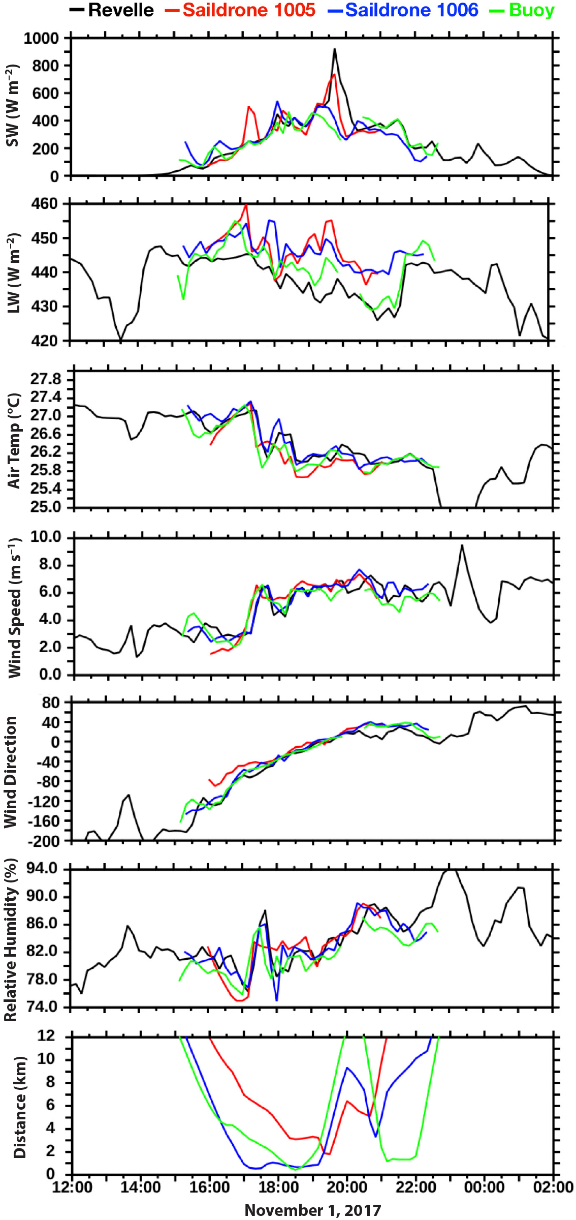
Figure 6. Saildrone 1005 (red), 1006 (blue), and WHOI buoy (green) versus R/V Revelle measurements (black) for SW and LW radiation, air temperature (Tair), wind speed and direction, and relative humidity (RH). Wind and Tair/RH all adjusted to 10 m. Also shown are the distances between R/V Revelle and saildrone 1005 (red), saildrone 1006 (blue), and the WHOI buoy (green).  > High res figure

 

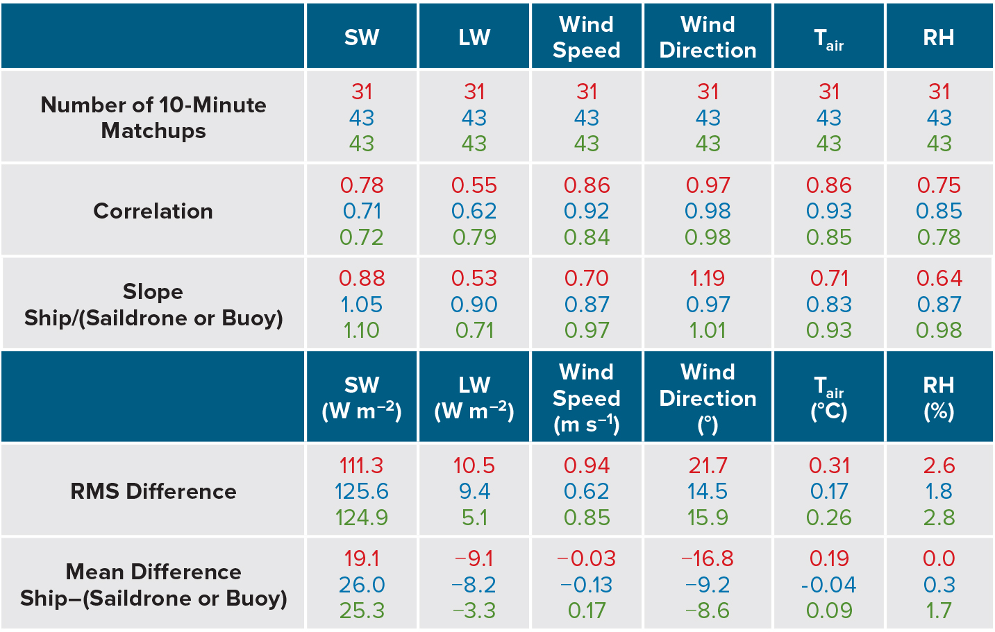
Table 2. Comparison of SD1005, SD1006, and WHOI ASIMET data with R/V Revelle measurements when the saildrones and buoy were within 12 km of the ship’s location. Wind, air temperature (Tair), and relative humidity (RH) measured by all platforms were adjusted to 10 m height. Saildrone short wave radiation measurements are tilt-corrected. SW = Shortwave radiation. LW = Longwave radiation. > High res table

 

This short period of ship-saildrone-buoy comparison highlights the instant measurement differences due to the distance between platforms. The RMS differences of SW radiation are large (>100 W m^–2). However, when Revelle is close to the saildrones and the buoy (within 5 km from 18:00 to 19:00; Figure 6), their differences from shipboard measurements are significantly reduced to 11–18 W m^–2, within the 20 W m^–2 instantaneous error of ASIMET. While the sample size of six 10-minute data points is too small to show the significance of the agreement, it is clear that natural spatial variability, as well as measurement errors, contributed to these differences between platforms. It is interesting to note that the mean difference (19–26 W m^–2) of the six-hour intercomparison is consistent with the RMS difference (26 W m^–2) in a ship-buoy comparison in the eastern tropical Pacific based on the six-hourly data when ship and buoy were within 10 km (Cronin et al., 2006).

As in the saildrone-buoy comparison, the LW radiation measurements of saildrones and the WHOI buoy have the lowest correlation with the shipboard measurements, though still above 95% significance level, assuming the matchups are independent. However, their mean and RMS differences range from 3 W m^–2 to 10 W m^–2, close to the ASIMET instant error of 7.5 W m^–2. In comparison, the RMS difference of six-hourly ship and buoy LW radiation in Cronin et al. (2006) is 6 W m^–2. Both wind speed and wind direction are highly correlated between compared platforms. The mean wind speed differences are close to the mean error of ASIMET 0.1 m s^–1, while the RMS differences are much larger than the instant error of ASIMET 0.1 m s^–1 (more in low winds) but more consistent with the ship-buoy RMS difference of six-hourly data (0.8–1 m s^–1) in Cronin et al. (2006). The mean and RMS differences in wind direction are about the same, likely due to the limited sample size, and they are larger than the instant (6°, more in low wind) and mean (5°) ASIMET error. However, the wind was changing dramatically during the six-hour intercomparison, from weak northerly to stronger easterly and then southerly. The wind direction uncertainties are therefore much smaller than the true signal of a 180° turn (Figure 6). This subsynoptic weather system with rotating wind and its associated clouds likely contributed to the large differences in SW and LW measurements by different platforms that are separated by some distance. Similar to the saildrone-buoy comparison, among all the measured variables, the air temperature and relative humidity measurements are closest to the shipboard measurements, with mean and RMS differences within the specified mean and instant ASIMET standard errors.

 

Summary and Conclusion

The saildrone is a new unmanned, long-​endurance surface vehicle that can be launched from shore and reach remote areas of the world ocean on its own without the need for ship time. One of the primary goals of the pilot study discussed here was to evaluate the saildrone as a potential platform for the Tropical Pacific Observing System to monitor surface air-sea interaction and biogeochemistry in a variety of sampling modes (e.g., adaptive, stationary, repeat section). As a first step, saildrone measurements were compared to field-proven technology to determine whether their accuracies could meet EOV and ECV requirements.

To accomplish this, two saildrones were launched from San Francisco, California, to participate in the SPURS-2 field campaign for validation of saildrone measurements against the SPURS-2 central buoy ASIMET and R/V Roger Revelle measurements, which have a long history of success in observing air-sea fluxes, and well-known accuracy documented by previous analyses (Colbo and Weller, 2009; Bigorre et al., 2013).

The intercomparison of saildrone and WHOI buoy ASIMET measurements is very encouraging (Figures 4 and 5, Table 1). The ship-saildrone-buoy comparison reveals the agreement and instantaneous differences between platforms in relation to separation distance and a passing subsynoptic weather system. Given the short duration of the ship-buoy-saildrone comparison, the agreement between all platforms is reasonably good, and is consistent with the ship-buoy comparison conducted during the Eastern Pacific Investigation of Climate Processes (Cronin et al., 2006). This validation suggests that the saildrone can be a valuable autonomous platform for observing air-sea surface heat and momentum fluxes (through bulk algorithm) in the tropical Pacific.

Saildrone navigation in the low wind and strong current conditions of the tropics has been mostly successful. The two saildrones were able to stay on track most of the time, but on two occasions, during October 19–21 and November 10–11, they were swept off track by strong currents in low wind conditions.

The saildrone is an attractive platform because its navigational response allows adaptive sampling. Cheaper than research vessels, it offers an advantage for long-term monitoring of the atmosphere and surface ocean in remote areas of the world ocean. However, future use of saildrones in both process studies and monitoring will need to take into account the impacts of local winds and currents in mission planning. Use of multiple saildrones will help to achieve better coverage and objective mapping of the processes to be observed even when the saildrones are temporarily off track because of adverse wind/current conditions.

Close coordination with other platforms (ships, floats, and moored buoys) such as in SPURS-2 is necessary not only for improved capability in observing complex multiscale, multiprocess air-sea interaction but also for intercalibration of sensors. Almost all ocean observation sensors are subject to drift. Rendezvous of different platforms for sensor calibration will help to improve the quality of climate observations. Salinity, the central variable studied during SPURS-2, is challenging to measure and is especially prone to drift due to biofouling. During SPURS-2, the newly calibrated CTDs on the saildrones helped to identify the salinity drift of the surface layer CTD sensors on the central WHOI buoy. However, just two weeks after SPURS-2, the Citadel CTDs on the saildrones began to show large drift compared to their SBE CTDs. We therefore recommend that saildrones and other USVs should devote at least one day to circumnavigating moored reference buoys whenever possible during different stages of their missions to characterize the status of the sensors on both USVs and buoys. Within observing networks, saildrones could be used for ongoing sensor intercomparisons linking data quality on different platforms.

Through this study, the saildrone has been shown to be a promising new platform for observing air-sea interaction processes in remote ocean locations. In order to become a mature ocean observing platform for GOOS, validation and additional demonstration missions must be performed under a wide range of field conditions (Lindstrom et al., 2012). Special attention needs to be paid to the downwelling SW and LW radiation measurements, which tend to have relatively larger RMS differences (or instantaneous errors) for SW and lower correlation for LW radiation between platforms than the other compared variables.

Zhang, D., M.F. Cronin, C. Meinig, J.T. Farrar, R. Jenkins, D. Peacock, J. Keene, A. Sutton, and Q. Yang. 2019. Comparing air-sea flux measurements from a new unmanned surface vehicle and proven platforms during the SPURS-2 field campaign. Oceanography 32(2):122–133, https://doi.org/10.5670/oceanog.2019.220.

Badosa, J., J. Wood, P. Blanc, C.N. Long, L. Vuilleumier, D. Demengel, and M. Haeffelin. 2014. Solar irradiances measured using SPN1 radiometers: Uncertainties and clues for development. Atmospheric Measurement Techniques 7:4,267–4,283, https://doi.org/10.5194/amt-7-4267-2014.
1. Bigorre, S.P., R.A. Weller, J.B. Edson, and J.D. Ware. 2013. A surface mooring for air-sea interaction research in the Gulf Stream: Part II. Analysis of the observations and their accuracies. Journal of Atmospheric and Oceanic Technology 30:450–469, https://doi.org/10.1175/JTECH-D-12-00078.1.
2. Cokelet, E.D., R. Jenkins, C. Meinig, N. Lawrence-Slavas, C.W. Mordy, P.J. Stabeno, H. Tabisola, and J.N. Cross. 2015. The use of saildrones to examine spring conditions in the Bering Sea: Instrument comparisons, sea ice meltwater and Yukon River plume studies. Paper presented at Oceans’15 MTS/IEEE, Marine Technology Society and Institute of Electrical and Electronics Engineers, October 19–22, 2015, Washington, DC.
3. Colbo, K., and R.A. Weller. 2009. The accuracy of the IMET sensor package in the subtropics. Journal of Atmospheric and Oceanic Technology 9:1,867–1,890, https://doi.org/​10.1175/2009JTECHO667.1.
4. Cravatte, S., W.S. Kessler, N. Smith, S. Wijffels, K. Ando, M. Cronin, T. Farrar, E. Guilyardi, A. Kumar, T. Lee, and others. 2016. TPOS 2020 Project: First Report. GOOS-215, TPOS 2020, 200 pp., http://tpos2020.org/first-report/.
5. Cronin, M.F., C.W. Fairall, and M.J. McPhaden. 2006. An assessment of buoy-derived and numerical weather prediction surface heat fluxes in the tropical Pacific. Journal of Geophysical Research 111, C06038, https://doi.org/10.1029/2005JC003324.
6. Cronin, M.F., N.A. Pelland, S.R. Emerson, and W.R. Crawford. 2015. Estimating diffusivity from the mixed layer heat and salt balances in the North Pacific. Journal of Geophysical Research 120(11):7,346–7,362, https://doi.org/​10.1002/2015JC011010.
7. Emond, M., D. Vandemark, J. Forsythe, A.J. Plueddemann, and J.T. Farrar. 2012. Flow Distortion Investigation of Wind Velocity Perturbations for Two Ocean Meteorological Platforms. Woods Hole Oceanographic Institution Technical Report, WHOI-2012-02, 66 pp.
8. Edson, J.B., V. Jampana, R.A. Weller, S.P. Bigorre, A.J. Plueddemann, and C.W. Fairall. 2013. On the exchange of momentum over the open ocean. Journal of Physical Oceanography 43(8):1,589–1,610, https://doi.org/​10.1175/JPO-D-12-0173.1.
9. Fairall, C.W., E.F. Bradley, J.E. Hare, A.A. Grachev, and J.B. Edson. 2003. Bulk parameterization of air-sea fluxes: Updates and verification for the COARE algorithm. Journal of Climate 16(4):571–591, https://doi.org/10.1175/1520-0442(2003)016​<0571:​BPOASF>2.0.CO;2.
10. Farrar, J.T., and A.J. Plueddemann. 2019. On the factors driving upper-ocean salinity variability at the western edge of the Eastern Pacific Fresh Pool. Oceanography 32(2):30–39, https://doi.org/​10.5670/oceanog.2019.209.
11. Lindstrom, E., J. Gunn, A. Fischer, A. McCurdy, and L.K. Glover. 2012. A Framework for Ocean Observing. Task Team for an Integrated Framework for Sustained Ocean Observing. Paris, France, UNESCO, IOC/INF-1284, 25 pp., https://doi.org/​10.5270/OceanObs09-FOO.
12. Long, C.N., A. Bucholtz, H. Jonsson, B. Schmid, A.M. Vogelmann, and J. Wood. 2010. A method of correcting for tilt from horizontal in downwelling shortwave irradiance measurements on moving platforms. The Open Atmospheric Science Journal 4:78–87, https://doi.org/​10.2174/​1874282301004010078.
13. McPhaden, M.J., A.J. Busalacchi, R. Cheney, J.-R. Donguy, K.S. Gage, D. Halpern, M. Ji, P. Julian, G. Meyers, G.T. Mitchum, and others. 1998. The Tropical Ocean Global Atmosphere (TOGA) observing system: A decade of progress. Journal of Geophysical Research 103:14,169–14,240, https://doi.org/​10.1029/97JC02906.
14. Meinig, C., R. Jenkins, N. Lawrence-Slavas, and H. Tabisola. 2015. The use of saildrones to examine spring conditions in the Bering Sea: Vehicle specification and mission performance. Paper presented at Oceans’15 MTS/IEEE, Marine Technology Society and Institute of Electrical and Electronics Engineers, October 19–22, 2015, Washington, DC.
15. Meinig, C., E.F. Burger, N. Cohen, E.D. Cokelet, M.F. Cronin, J.N. Cross, S. De Halleux, R. Jenkins, A.T Jessup, C.W. Mordy, and others. In press. Public private partnerships to advance regional ocean observing capabilities: A saildrone and NOAA-PMEL case study and future considerations to expand to global scale observing. Review Article for Oceanobs19: An Ocean of Opportunity. Frontiers in Marine Science.
16. Send, U., R. Weller, D. Wallace, F. Chavez, R. Lampitt, T. Dickey, M. Honda, K. Nittis, R. Lukas, M. McPhaden, and R. Feely. 2010. “OceanSITES” in Proceedings of OceanObs’09: Sustained Ocean Observations and Information for Society (Vol. 2). Venice, Italy, September 21–25, 2009, J. Hall, D.E. Harrison, and D. Stammer, eds, ESA Publication WPP-306, https://doi.org/10.5270/OceanObs09.cwp.79.
17. Sutton, A.J., C.L. Sabine, S. Maenner-Jones, N. Lawrence-Slavas, C. Meinig, R.A. Feely, J.T. Mathis, S. Musielewicz, R. Bott, P.D. McLain, and others. 2014. A high-frequency atmospheric and seawater pCO₂ data set from 14 open-ocean sites using a moored autonomous system. Earth System Science Data 6:353–366, https://doi.org/10.5194/essd-6-353-2014.
18. Zhang, D., M.F. Cronin, X. Lin, R. Inoue, A. Fassbender, S. Bishop, and A. Sutton. 2017. Observing air-sea interaction in the western boundary currents and their extension regions: Considerations for OceanObs’19. US CLIVAR Variations 15(4):23–30.

This is an open access article made available under the terms of the Creative Commons Attribution 4.0 International License (https://creativecommons.org/licenses/by/4.0/), which permits use, sharing, adaptation, distribution, and reproduction in any medium or format as long as users cite the materials appropriately, provide a link to the Creative Commons license, and indicate the changes that were made to the original content. Images, animations, videos, or other third-party material used in articles are included in the Creative Commons license unless indicated otherwise in a credit line to the material. If the material is not included in the article’s Creative Commons license, users will need to obtain permission directly from the license holder to reproduce the material.