Introduction
The resonant response of the ocean to wind forcing produces enhanced variability in currents near the Coriolis frequency (also called the inertial frequency). Although the wind drives currents and vertical mixing directly, the ocean’s stratification limits these phenomena to a relatively thin surface layer over which properties and momentum are homogenized—a “mixed layer” typically 10–50 m thick at the top of the 3,000–5,000 m deep stratified ocean. The mechanisms that allow these mixed-layer currents to influence the deeper ocean were the subject of the 2018–2020 Near-Inertial Shear and Kinetic Energy in the North Atlantic Experiment (NISKINe) south of Iceland, a Departmental Research Initiative (DRI) led by the Physical Oceanography Program of the Office of Naval Research (ONR) (Thomas et al., 2020, and 2024, in this issue; Asselin et al., 2020; Raja et al., 2022; Kunze et al., 2023). In particular, the ability of horizontal gradients in the mixed-layer currents to produce vertical motions through horizontal convergence and divergence, thereby forcing vertically propagating near-inertial internal waves, was of considerable interest, as was the subsequent dissipation of this propagating energy in the water column (Kunze et al., 2023).
The leading theory for explaining internal-wave-mesoscale interactions is vorticity refraction as described recently by Thomas et al. (2020) and Asselin et al. (2020), following Kunze (1985), and many since, using WKB (Wentzel-Kramers-Brillouin) internal wave ray tracing. Essentially, this is the tendency for the mesoscale vorticity field to steer the horizontal propagation direction of near-inertial wave energy down vorticity gradients, decrease the horizontal scale of the waves, and increase their downward group velocity, resulting in a transformation from long-wavelength inertial oscillations in the mixed layer to smaller-scale downward-propagating near-inertial waves in the thermocline. The planetary vorticity gradient (β) can produce the same set of effects (Anderson and Gill, 1979; D’Asaro, 1989; Garrett, 2001), and evaluating the relative impact of different vorticity scales was a key goal of NISKINe (Thomas et al., 2024, in this issue).
In principle, all the ingredients needed for internal wave forcing and dynamics are present in numerical forecast models of the ocean and atmosphere (Müller et al., 2015; Nelson et al., 2020; Arbic, 2022; Raja et al., 2022), and many of the important forcing and surface-ocean environmental properties, including currents, winds, and water temperature, can be observed by satellite. Global estimates of near-inertial wind energy input (e.g., Rimac et al., 2013; Alford, 2020; Raja et al., 2022) and the relationship between near-inertial energy and mesoscale eddy vorticity (e.g., Elipot et al., 2010) have been made using these types of datasets. However, the O(10 km) horizontal scales in currents and oceanic boundary layer thickness that are thought to dominate the interaction between the environment and internal waves are not yet well resolved by either models or satellite measurements, making in situ characterization of both the horizontal structure of the background and the waves of special importance for this study. A similar approach has been taken previously in mooring-based (Weller, 1982; D’Asaro et al., 1995) and ship survey-based (D’Asaro and Perkins, 1984; Kunze and Sanford, 1984, 1986; Kunze et al., 1995; Kunze, 1986; Kunze and Toole, 1997) studies, as well as more recently with Lagrangian arrays similar to those described here (Lien and Sanford, 2019; Kunze et al., 2021; Essink et al., 2022).
We report on a subset of the focused suite of measurements from the June 2019 NISKINe process cruise on R/V Neil Armstrong. The measurements were collected in the Iceland Basin along one of the principal pathways for the flow of warm, salty subtropical water into the subpolar gyre (Figure 1a) via the North Atlantic Current (NAC). During the cruise period, the study region was characterized by moderate wind forcing, together with strong eddy structures, and property gradients associated with the NAC. The location is near a local maximum in climatological mesoscale eddy variability due to the growing and evolving meanders and instability of the NAC, but that growth is limited by ridges bounding the basin to the east and west (Figure 1). A variety of shipboard and autonomous platforms observed inertial oscillations at the surface and near-inertial waves below the surface, with a key observational challenge being to capture lateral gradients in currents and their variability both above and below the inertial frequency over multiple inertial cycles. Later phases of the project included long-duration measurements to characterize seasonal variability using profiling floats (Kunze et al., 2023) and moorings (Voet et al., 2024, in this issue).
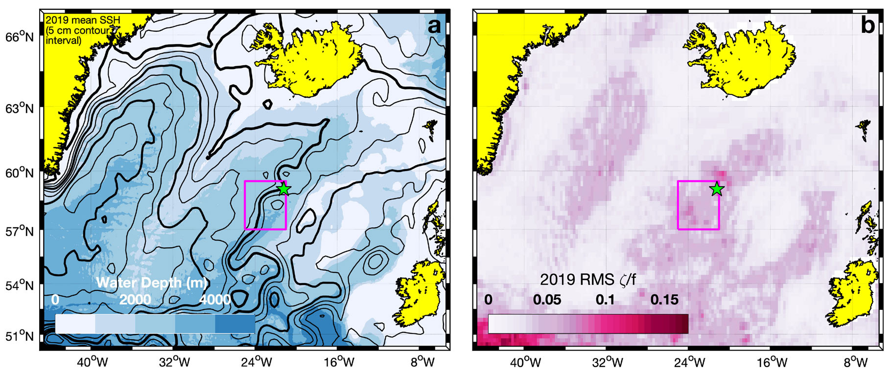
FIGURE 1. Mesoscale circulation and vorticity in the eastern subpolar North Atlantic. (a) Sea-surface height (SSH) contours from AVISO mapped altimetry (2019 mean). Thick contours are every 20 cm and thin contours every 5 cm over shaded bathymetry (1,000 m contour interval). SSH contours are streamlines of the surface geostrophic flow and illustrate the splitting of the northeastward-flowing North Atlantic Current (NAC) into separate branches recirculating to the west in the Subpolar Gyre or continuing northward across the Greenland–Scotland Ridge. (b) Root-mean-squared (RMS) variance of 2019 AVISO ¼° first-differenced vorticity (ζ) normalized by planetary vorticity (f), emphasizing bands of mesoscale variability associated with the northeastward branches of the NAC (panel a) in the three eastern subpolar gyre basins (left to right, Irminger Sea, Iceland Basin, and Rockall Trough). The magenta box and green star in both panels indicate the NISKINe float deployment region (Figure 2d) and mooring location (Voet et al., 2024, in this issue), respectively. > High res figure
|
Methods
In order to measure the horizontal gradients in both subinertial (geostrophic) and superinertial (internal wave) horizontal currents and density, three arrays of autonomous profiling floats were deployed from Armstrong in June 2019—mostly in and around an anticyclonic (clockwise rotating) eddy centered at 58°N, 22.3°W (Figure 2).
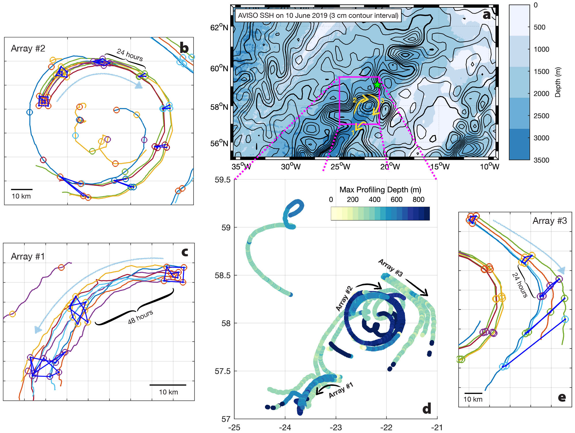
FIGURE 2. NISKINe EM-APEX trajectories and array shapes during the 2019 process cruise. (a) Mid-cruise (June 10, 2019) SSH snapshot, showing a chain of NAC eddies in the Iceland Basin and approximate trajectories of the three arrays relative to an anticyclone (clockwise eddy). (d) Expanded view of the cruise region (magenta box in panel a), with trajectory and maximum profiling depth of all EM-APEX floats during the 2019 process cruise period. Individual arrays are highlighted in the outer three panels (b, c, and e), with trajectories (interpolated from surface GPS positions to a common ½-hour time grid) colored by float. Symbols mark the positions of all floats in the array at 48-hour intervals for Array 1 and at 24-hour intervals for Arrays 2 and 3. A subset of connecting lines is shown for each array to illustrate deformation and relative advection. > High res figure
|
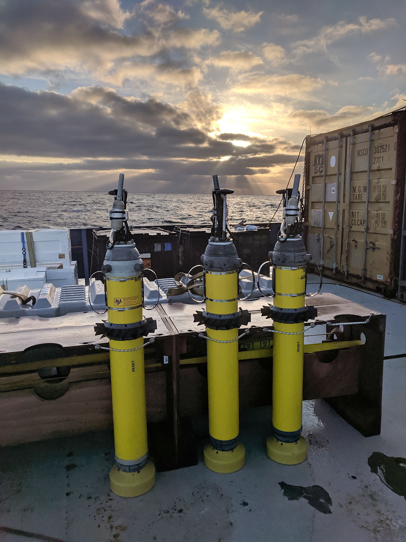
EM-APEX (Electro-Magnetic Autonomous Profiling EXplorer) profiling floats were used. These are similar to the profilers used in the global Argo array but with the addition of a velocity measurement using the electric currents generated by the movement of conducting seawater in Earth’s magnetic field (Sanford et al., 2005, 2007). All floats were also equipped with fast-response FP07 temperature microstructure sensors for the estimation of turbulent mixing levels (Lien et al., 2016). The microstructure measurements have been presented by Kunze et al. (2023), while this paper focuses on the velocity structure of near-inertial waves.
Temperature and salinity profiles from the Sea-Bird 41CP CTD on the EM-APEX (accurate to 0.001°C and 0.001 psu for the purposes of the gradients needed for this study) are used to compute density with the EOS-80 algorithm (accurate to 0.001 kg m–3; Millero et al., 1980).
The floats mainly cycled between 400 m and the surface, making round-trip excursions approximately every 2.5 hours. Floats that went deeper sampled proportionately less frequently (see Figure 2d for profiling depths). Array 1 included eight floats and remained in the water for four days, Array 2 also included eight floats and remained for seven days (though four of the floats were recovered about halfway through), and Array 3 included four floats profiling for three days. In all cases, the array duration spanned multiple 14-hour inertial cycles, allowing a frequency-domain separation of internal wave and geostrophically balanced contributions.
Because wind forcing of the NISKINe region was primarily by atmospheric phenomena (e.g., storms) larger than the experimental domain, we use a simple “slab” model of the upper ocean (Pollard and Millard, 1970) to interpret the amplitude and phase of the near-inertial currents (Figure 3). The slab model solves for the time-varying velocity (u(t), v(t)) of a mixed layer with constant thickness h and density ρ under Coriolis acceleration, forced by wind stress (τx(t), τy(t)), and damped by a linear drag r:
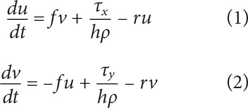
where f = 1.23 × 10⁻⁴ s–1 is the inertial frequency at 58°N latitude. The slab thickness, h, is set to the average of the observed thickness (with the mixed layer base defined as the point where density increases to greater than 0.1 kg m–3 above the shallowest measured value). Wind stress τ = ρairCDu2wind is derived from ship wind speed measurements (Figure 3) using a constant quadratic drag coefficient CD = 1.4 × 10⁻³. The linear damping coefficient that gives a decent match to observations is r = 4 × 10⁻⁶ s–1, making the model response relatively insensitive to the winds more than three days prior to any point.
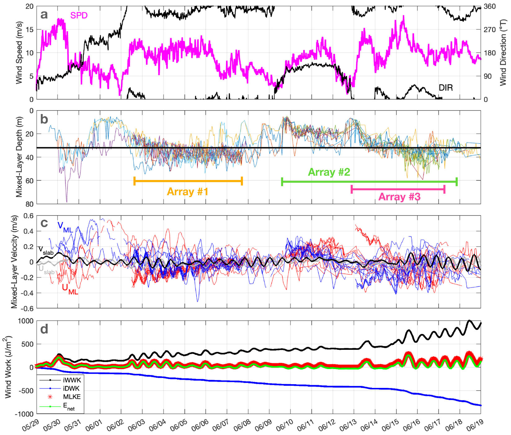
FIGURE 3. Wind forcing and near-inertial mixed-layer response in the NISKINe region, as estimated from a “slab” model of mixed-layer currents (Pollard and Millard 1970; Alford, 2001) with a damping timescale of three days (Equations 1 and 2). Panels show (a) wind speed and direction (upwind direction east of north) measured from R/V Armstrong, (b) mixed-layer thickness measured by all EM-APEXes, colored by float, with the median value of 32 m used in the slab model shown as a horizontal black line and the deployment periods of the three arrays labeled with horizontal bars, and (c) mixed-layer currents measured by EM-APEX floats (U: red; V: blue) and simulated by the wind-forced slab model (U: gray; V: black). Panel (d) shows slab-model kinetic energy (red), and energy terms: integrated wind-work (black), loss to drag (blue, with linear drag, r, serving as a proxy for a number of real-world processes including internal wave radiation and turbulent dissipation), and their sum (green) as a test on numerical accuracy. > High res figure
|
For analysis of internal wave motions, the observed mixed-layer velocity time series is high-passed by subtracting a one-day Gaussian-weighted running mean. The result is then a composite of all internal wave band motions, including the broad near-inertial peak (Figures 4a and 5a). The subtracted low-passed time series is used to represent the geostrophically balanced mesoscale velocity field. The time series of array-scale vorticity is estimated from two-dimensional plane fits to this low-passed velocity (Figures 4d and 5d).
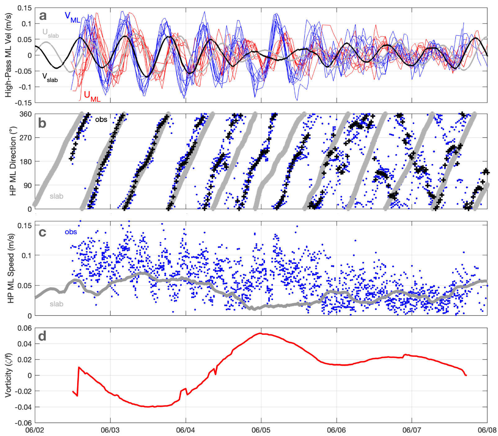
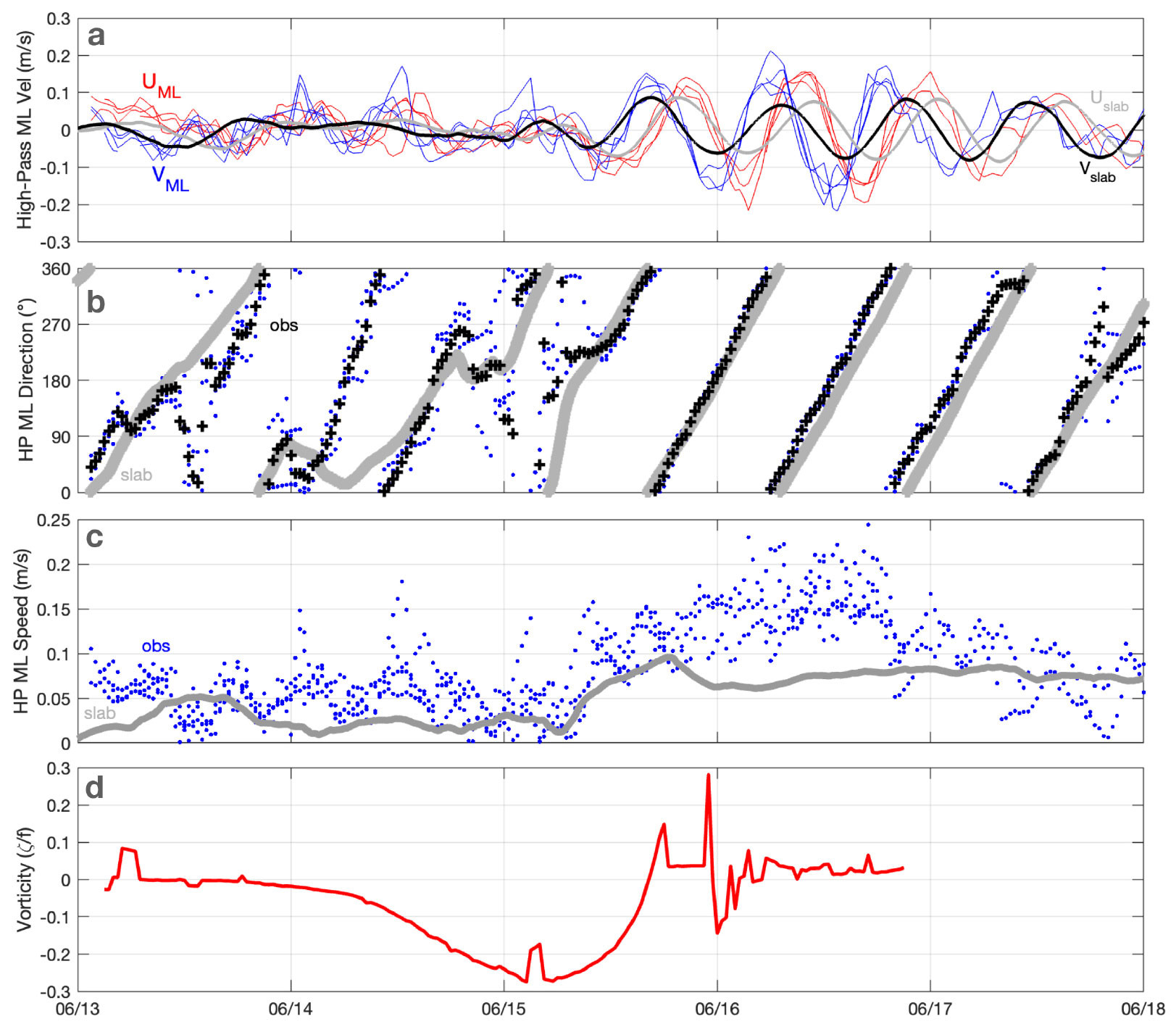
FIGURE 4. Array 1 time series, illustrating the degree of coherent near-inertial response as seen in high-passed mixed-layer (HP ML) (a) velocity components (U: east and V: north, with red and blue from EM-APEX observations; gray and black from slab model), (b) direction (degrees east of north, with slab model gray, individual measurements blue and array mean black), and (c) speed (observations in blue and slab model in gray). (d) Low-frequency vorticity estimated from two-dimensional plane fits to the low-frequency mixed-layer velocity across the array. > High res figure
|
Near-inertial parameters (i.e., clockwise-rotating current amplitude and phase) determined from inertial-frequency sinusoid fits to the temporal variability sampled by each float over 28-hour windows (two inertial periods) are also used to compute horizontal phase gradients from two-dimensional plane fits on depth levels. The slope and direction of the inertial phase gradient yield, respectively, the horizontal wavelength and horizontal propagation direction of a best-fit near-inertial wave (Figures 6 and 7). The fraction of phase (ϕ) variance explained by the plane fit R2 = <ϕ2plane>/<ϕ2data> is an attempt to evaluate the goodness of fit.
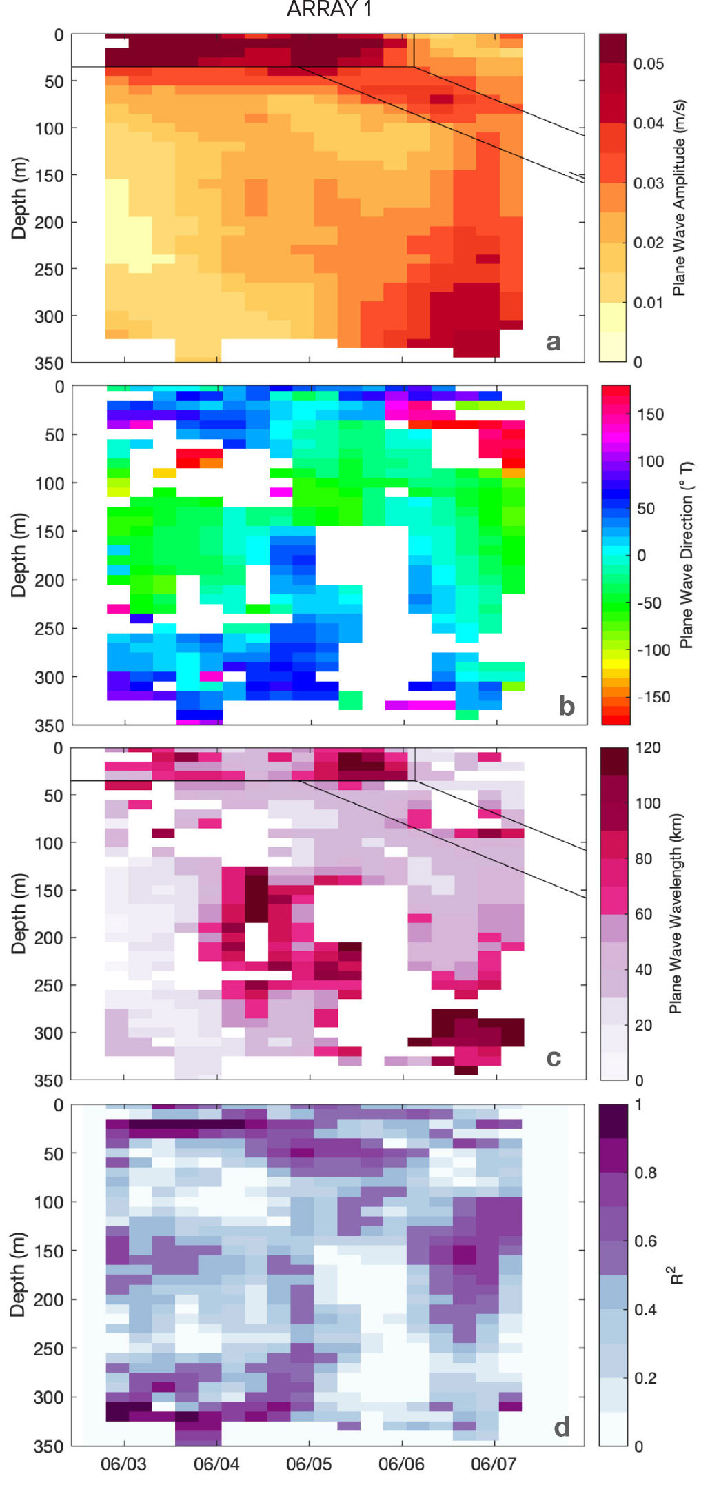
FIGURE 6. Profile time series of horizontal near-inertial plane-wave parameters at Array 1. Quantities plotted are derived from linear horizontal plane fits to the parameters from clockwise-in-time inertial cycle fits at each float: (a) near-inertial amplitude in m s–1, (b) propagation direction (toward) in degrees east of north, (c) horizontal wavelength in kilometers, and (d) goodness-of-fit parameter R2. Depth-time values with R2 < 0.2 are masked out in panels b and c. Solid black lines in panels a and c delineate averaging regions discussed in the Discussion section (and are intended to represent the mixed-layer oscillation and the descending internal wave beam). > High res figure
|
Results
The relationship between the observed high-passed mixed-layer currents and the wind-forced slab model is shown in Figures 4 and 5 for Arrays 1 and 3, with some notes on the different behaviors at the three arrays as follows:
Array 1
Array 1 was deployed in two nested boxes south of the mesoscale eddy dipole targeted for observation by the process cruise (Thomas et al., 2020; Figure 2). Inertial oscillations were initially coherent across the full array of eight floats and closely aligned with the slab model predictions (Figure 4b) before drifting apart over two days due to a positive frequency shift of ~12%. The wind forcing that produced this inertial motion was strongest about three days before the array launch but received a small additional kick from an increase in speed and shift in direction at the time of launch (Figure 3a).
One aspect of the observed mixed-layer currents not captured by the slab model is the difference in amplitude between the vector components, with v exceeding u by 30%–50% (Figure 4a), resulting in a north-south oriented ellipticity in the rotating currents (and also appearing as a wiggle in the direction [Figure 4b] and a pulsing in the speed [Figure 4c] at about twice the inertial frequency). This feature will need further investigation to explain but could be related to the presence of higher-frequency motions—for example, a semidiurnal internal tide or other preexisting northward or southward-propagating internal wave. Near-inertial ellipticity can be enhanced at the boundaries or by mesoscale baroclinicity (sloping isopycnals; Mooers, 1975; Kunze, 1985; Whitt and Thomas, 2013). Linear internal waves would suggest v/u ~ ω/f, so the frequency shift of 12% mentioned above is insufficient to explain the observed ellipticity.
As the mesoscale eddy field evolved (with the core of the anticyclone moving northward), the currents advecting the array weakened and changed direction, taking the array westward and then southward instead of northward through the dipole’s central jet. This change was apparent in shipboard ADCP current observations shortly after array launch, and eventually from satellite altimetry as well, but the lack of temporal and spatial sea surface height and current coverage made this aspect of the ongoing NAC meander evolution impossible to predict. Additionally, the box formation of the array was immediately deformed by small-scale horizontal shear, with the eight floats trading places in random fashion while the cluster as a whole remained fairly compact. The inner 1 km box spread rapidly, while the outer 3 km box maintained its approximate spacing. The final ~3 km bulk spread of the floats after four days was not much larger than the initial 2 km average spacing.
Three days after launch, the amplitude of the measured near-inertial currents had decreased, and phase had become essentially random (Figure 4a–c), while the array geometry (overall spacing and spread) had not changed dramatically (Figure 2c). Mesoscale vorticity as seen in the array trajectory curvature was weak but generally positive. Vorticity on the ~5 km scale of the array, determined from plane-fits to the measured subinertial velocities (Figure 4d) as well as the rotation of the array, was initially negative and then switched to positive. It is possible that the initial negative vorticity facilitated the retention of coherent near-inertial oscillations, while the later positive vorticity led to a dispersal of near-inertial wave energy (Kunze, 1985). The array did not maintain its two-box shape for more than a day but was instead scrambled by a combination of 1–3 km lateral gradients and differences in float motion due to profiling behavior (vertical speed, surface time, etc.) in a vertically sheared velocity field—although the float programming attempted to minimize the latter. Disentangling the contributions to the float trajectories is the subject of ongoing work. The rate and randomness of this scrambling is more apparent in Array 1 than in Arrays 2 and 3, which may be the result of the stronger influence of advection and straining by large-scale gradients, along with weaker small-scale shears, at the latter locations.
Profile time series of wave properties estimated from horizontal plane fits to Array 1 near-inertial parameters show energy extending downward over time from the 40 m deep mixed layer to about 100 m (Figure 6a). Coincident with this downward extension, deeper energy appears at 100–300 m depth following the surface forcing and the greatest amplitudes in the surface layer. This may be due to horizontal propagation from outside the array. Subsurface horizontal wavelengths in the descending beam (Figure 6c) are somewhat smaller (~50 km) than mixed-layer wavelengths (~65 km). However, the deeper energy has a longer wavelength similar to that at the surface and may indicate the direct forcing of lower-mode energy rather than a downward wave radiation. Interpretation is complicated by the changing array geometry and the sometimes unstable output from the plane fits. R2 is an imperfect metric, being elevated when fewer floats (down to a minimum of four) are used in the fit and reduced when the observed gradient is weak (because the fit accounts for less of the data variance). Furthermore, when the array is distorted into a line, only one direction of gradient can be evaluated, and the plane fit only provides a lower limit on horizontal wavenumber.
Array 2
Array 2 also began as a nested box, this time profiling to 500 m depth in order to capture more of the mesoscale structure (Figure 2). This resulted in less frequent sampling (though still resolving the inertial frequency with ~3-hour cycles) as well as slower advection and a relatively small increase in the geometric spread of the array (at least initially). Compared to Array 1, the overall deformation of Array 2 was more easily described as a coherent rotation and straining while orbiting the anticyclonic mesoscale (though still small) eddy—the eastern member of the dipole described by Thomas et al. (2020). Vorticity across the array was negative and increased moderately with time. The difluent strain axis was oriented nearly along the tangential trajectory of the array. After three days, four of the floats in the array were recovered and redeployed to form Array 3, while the remaining four floats continued around the eddy. The overall strain rate increased as the array dispersed.
Observed near-inertial mixed-layer motions in Array 2 (Figure 3c, June 10 and onward) were somewhat stronger than those predicted by the slab model (at least in part because the mixed layer was initially thinner than the constant value used in the model). Detailed plots for this array are not included here because of the similarity of the near-inertial response to those seen in Arrays 1 and 3. Inertial phase (current direction) lined up well with the slab model during forcing events (and over much of the array deployment period), but higher-frequency (super-inertial) motion was evident in the form of a gradual departure of observed phase from the model (similar to Array 1 behavior at 06/03–06/06 in Figure 4b). Additional wind fluctuations near the end of the array deployment period increased the near-inertial amplitude and brought a convergence of phase, despite the large dispersion of the array by this time. Mixed-layer near-inertial fits (not shown) found the largest amplitudes in Array 2, accompanied by long horizontal wavelengths at the surface and shorter wavelengths at depth. An exception to this was a long-wavelength coherent wave observed at 200 m in the last few days directed toward the center of the anticyclone.
Array 3
Array 3 lost its coherent shape more quickly than the other two arrays in a region of strong velocity at the periphery of the anticyclonic eddy. Over the first two days, strain in the direction perpendicular to the trajectory deformed the array while preserving the arrangement of the floats. After this time, the array stretched out into a single line. While initially, vorticity estimated from the array was very small (Figure 5d), both array-scale fits and the bend in trajectory on the second day show that the majority of the floats moved more definitively into the anticyclone. However, the easternmost float was likely on track to depart the eddy entirely.
Because of weak, but still fluctuating, wind forcing in the first half of this array deployment (Figure 3c, June 13 and onward), slab-model current predictions rotated more slowly than at other times, with a markedly subinertial character (Figure 5b). In contrast, observed currents were stronger (Figure 5c) and retained inertial rotation (Figure 5b). At the end of the deployment, a wind increase brought observed and modeled inertial motions back together. As with coherent periods in both Arrays 1 and 2, the separation between observed and modeled near-inertial phase grew with time, indicating a super-inertial frequency in the real ocean that contrasts with the purely inertial slab model.
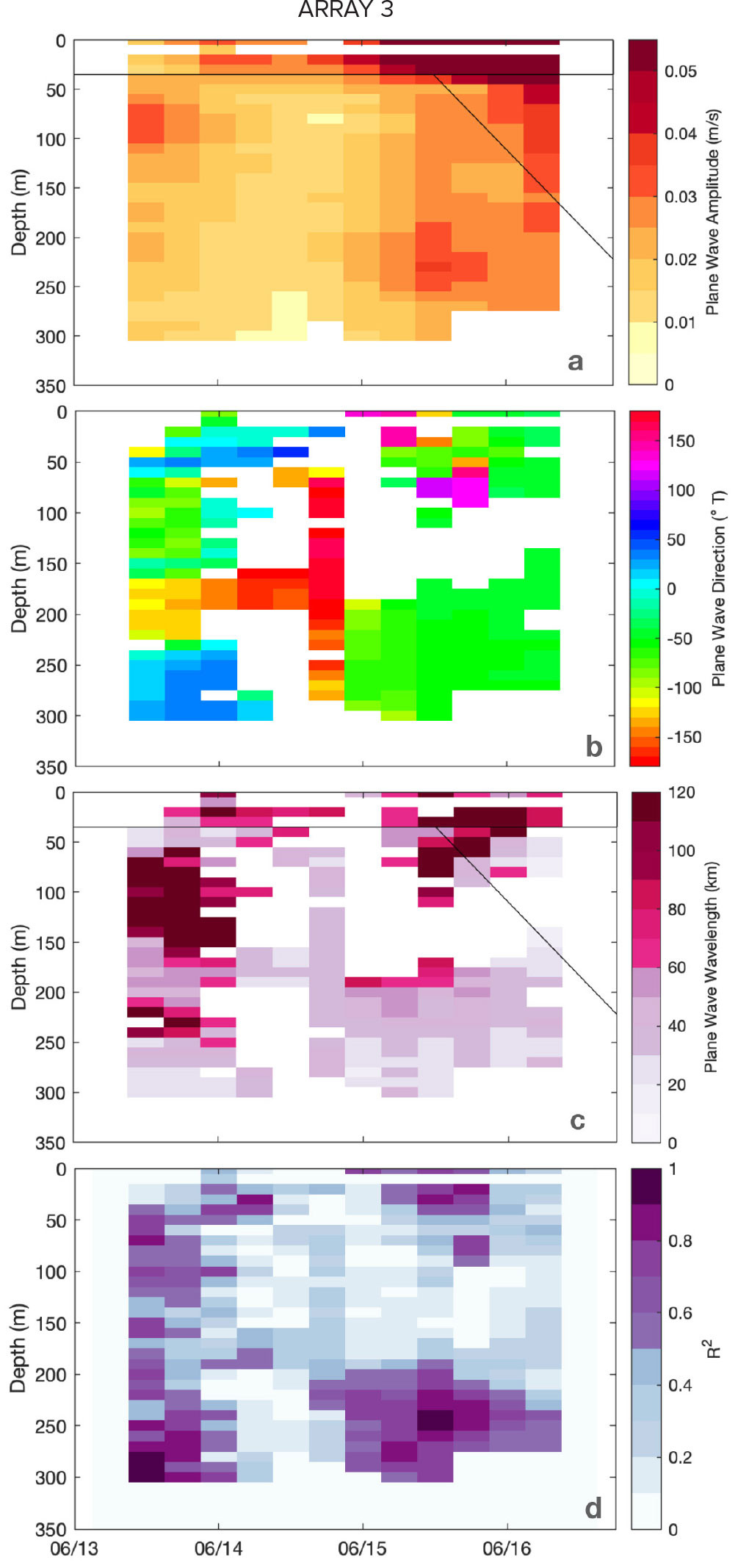
The plane-fitted inertial parameters at Array 3 (Figure 7) reveal several layers with different subsurface propagation characteristics, including a wave vector directed radially toward the center of the anticyclone (–60° to –90°, i.e., WNW) in the second half of the record at around 200 m depth (Figure 7b).
Discussion
Our observations of mixed-layer and deeper near-inertial oscillations were aimed at capturing their spatial structure and relationship to wind forcing. Because of the Lagrangian nature of the profiling float approach, measurement array geometry and dispersion, mesoscale vorticity, and near-inertial phase propagation are all potentially related and may vary in concert or in opposition. In addition, the small arrays of four to eight floats presented here always miss some aspects of the spatial structure. Nevertheless, the set of contrasting case studies highlights a number of observable aspects of the near-inertial wave generation process worthy of further investigation: Array 3 observed strong strain and strong advection, Array 2 weak strain and strong advection, and Array 1 weak strain and weak advection—emphasizing subarray-scale random motions. The more rapid penetration of near-inertial energy out of the mixed layer at Array 3, the evolution of spatial coherence in the near-inertial waves with minimal measurement location disruption at Array 2, and the contrasting responses to similar winds at the different locations of Arrays 2 and 3 provide scenarios for development and evaluation of conceptual models and analytical theory.
In the Array 1 case, the decoherence of mixed layer near-inertial phase over the small region covered by the array occurred at the same time as the re-arrangement of float positions within the array. Although the mechanism for these two things could be different, it seems likely that velocity gradients on 1–3 km scales were responsible for both. This also implies that the horizontal wavelength of the mixed-layer convergence forcing thermocline near-inertial waves shifted to similar scales.
The horizontal plane-fit diagnostics (Figures 6 and 7) are noisy (the result of trying to isolate the space-time evolution of a single oscillation in the presence of considerable background variability) but do reveal that: (a) the strongest near-inertial amplitudes during wind forcing in the mixed layer are often followed by increased amplitude in the water column below after a few days, (b) in many cases this subsurface energy has shorter horizontal scales than the mixed-layer (although the values are often unstable and scattered), and (c) horizontal phase propagation tends to be directed toward the nearby anticyclonic eddy, consistent with vorticity refraction (Kunze, 1985; Asselin et al., 2020; Thomas et al., 2020). To further clarify these assertions about the plane fits, horizontal wavelength and propagation direction were averaged in two time-depth regions delineated by thin black lines in Figures 6 and 7. The two regions were chosen to represent the mixed-layer near-inertial oscillation and the descending near-inertial internal wave beam, using the inertial amplitude (panel a) as a guide. Results are more or less in line with expectations, although only just significant relative to the 95% confidence limits (estimated as twice the standard error) reported here: Array 1 average wavelength decreases from 66±7 km in the mixed layer to 52±7 km below (directed toward –52±22°T, i.e., to the NW, away from the cyclonic path curvature), and Array 3 wavelength decreases from 130±44 km in the mixed layer to 64±34 km below (directed toward –80±34°T, or WNW toward the anticyclone).
Conclusions
We’ve described salient features of the near-inertial variability observed by EM-APEX arrays used in NISKINe, with a focus on the characteristics that can be captured purely by a small number of inertial-resolving upper-ocean cycling profilers over a few days. Deeper analyses of the dynamics and energy budgets are under way, but notable findings from the three array deployments so far include:
- Surface-layer near-inertial oscillations of large horizontal wavelengths accompany rapid wind changes. A simple mixed-layer slab model (Pollard and Millard, 1970) with a three-day damping timescale does a reasonable job of predicting the initial amplitudes and phases of these motions, provided an appropriate thickness is used for the slab layer (Figures 3c, 4a,b, and 5a,b).
- In a caveat to the above, because of mixed-layer deepening during wind events, initial mixed-layer high-passed current amplitudes are typically larger than the slab model’s near-inertial predictions (Figures 4c and 5c) but agree better after the mixed layer has reached its final thickness. The north-south ellipticity to the mixed-layer currents at the Array 1 site is not easily explained.
- Observed mixed-layer velocities rotate clockwise in time, with phases initially tracking the slab model predictions, but becoming more rapid than the inertial frequency in many cases. This super-inertial rotation is consistent with a finite horizontal wavelength internal wave generation process (e.g., due to horizontal gradients in wind forcing or mixed-layer depth). The frequency shift does not directly correspond to the array-estimated vorticity (Figures 4b,d and 5b,d), but the wave propagation direction does seem to be steered by vorticity gradients.
- Subsurface near-inertial energy modulation typically follows surface changes, indicating that at least part of the ocean’s response to the wind is to generate downward-propagating internal waves, for example through vorticity refraction decreasing horizontal wavelength and increasing vertical group velocity (D’Asaro, 1995; Kunze, 1985; Asselin et al., 2020; Thomas et al., 2020; Essink et al., 2022; Figures 6 and 7).
The observations presented here reveal the often-complex nature of near-inertial motions in the subsurface ocean while reinforcing their ubiquity. Surface-layer oscillations during and immediately after strong wind forcing are well characterized by the simplest of models but rapidly become less coherent once the wind dies. In possibly the most striking example, near-inertial phase is effectively randomized over less than a day in the location with the weakest mesoscale vorticity. In the presence of strong mesoscale vorticity features, the steering of energy down the vorticity gradient reinforces near-inertial wave refraction theory that may be successfully applied to large-scale model parameterizations.
The energy carried by near-inertial motions makes an important contribution to the global internal wave field, and interactions with the eddy field steer this energy to the ultimate sites of dissipation, whose characteristics are critical for the predictions of ocean mixing needed for ocean circulation and tracer transport modeling. Studies with coordinated arrays of autonomous instruments provide effective means for simultaneously observing the multiple temporal and spatial scales of these interactions and making quantitative tests of theory. However, because the eddy flow fields are complex and there are a multitude of near-inertial wave forcing and propagation scenarios, many more examples are needed.
Acknowledgments
This work was supported by ONR grant N00014-18-1-2598 for the NISKINe DRI. Engineer Avery Snyder was instrumental in preparing and testing the EM-APEX and executing the multiple array deployments and recoveries during the process cruise. Success in these efforts simultaneous with numerous other DRI activities was made possible by the expert coordination of Chief Scientist Luc Rainville, Captain Kent Sheasley, and the crew of R/V Neil Armstrong.