Global ocean models that admit mesoscale turbulence spontaneously generate a substantial interannual-to-multidecadal chaotic intrinsic variability in the absence of atmospheric forcing variability at these timescales. This phenomenon is substantially weaker in non-turbulent ocean models but provides a marked stochastic flavor to the low-​frequency variability in eddying ocean models, which are being coupled to the atmosphere for next-generation climate projections. In order to disentangle the atmospherically forced and intrinsic ocean variabilities, the OCCIPUT (OceaniC Chaos – ImPacts, strUcture, predicTability) project performed a long (1960–2015), large ensemble (50 members) of global ocean/sea ice 1/4° simulations driven by the same atmospheric reanalysis, but with perturbed initial conditions. Subsequent ensemble statistics show that the ocean variability can be seen as a broadband “noise,” with characteristic scales reaching multiple decades and basin sizes, locally modulated by the atmospheric variability. In several mid-latitude regions, chaotic processes have more impact than atmospheric variability on both the low-frequency variability and the long-term trends of regional ocean heat content. Consequently, certain climate-relevant oceanic signals cannot be unambiguously attributed to atmospheric variability, raising new issues for the detection, attribution, and interpretation of oceanic heat variability and trends in the presence of mesoscale turbulence.

Climatic Trends and Variability

The release of greenhouse gases (GHGs) into the atmosphere by human activities since the Industrial Revolution has increased the amount of heat stored in the climate system. Over the last five decades, more than 90% of this excess heat has been transferred to the ocean (Church et al., 2011; Rhein et al., 2013). The subsequent thermal expansion of seawater, together with the enhanced melting of glaciers and ice sheets, has induced most of the observed global mean sea level rise at a rate of 3 ± 0.4 mm yr^–1 since 1993 (Nerem et al., 2018). The Intergovernmental Panel on Climate Change’s Fifth Assessment Report (IPCC, 2013) concludes that human activities have very likely impacted the observed trends of other globally averaged climate indices, such as surface air temperature since 1951, sea level, and 0–700 m ocean heat content since the 1970s.

Such measures of likeliness are often based on the dispersion obtained within ensembles of Atmosphere-Ocean General Circulation Model (AOGCM) simulations, comprising, for instance, integrations of several AOGCMs (e.g., Coupled Model Intercomparison Project Phase 5, or CMIP5; Taylor et al., 2012), or several integrations of a given AOGCM subject to slight initial perturbations. Because the coupled atmosphere-ocean system is nonlinear, such small initial perturbations may grow, and ensemble members progressively decorrelate in spite of their identical dynamics and external forcings (i.e., specified GHG concentration increase, volcanic eruption time series, etc.). Averaging over all ensemble members yields time series of what may be called the forced variability (i.e., the deterministic response of all members to their common forcing). Subtracting this forced variability from each member then yields, for each member, what we will call the chaotic variability of the system under consideration, whose temporal evolution is uncorrelated among the members. The El Niño-Southern Oscillation (ENSO) is a well-known example of a chaotic mode of coupled variability¹.

¹ Zivkovic and Rypdal (2013) discuss the stochastic or chaotic nature of ENSO dynamics. For the sake of simplicity, in this paper we will label as chaotic the part of a system’s variability that has different phases in different ensemble members despite their identical deterministic equations and external forcing.

 

Oceanic Trends and Variability

The ocean has much greater heat capacity than the atmosphere: the large observed increase in ocean heat content (OHC) is associated with modest oceanic temperature increases, which must be monitored accurately. The long-term trend of OHC also has a complex, non-uniform, three-dimensional structure (e.g., Llovel et al., 2010; Rhein et al., 2013) set by ocean dynamics and ocean basin geometry. Monitoring the OHC trend thus requires a global array of three-​dimensional sensors; the Argo program has provided such a relatively dense array since the 2000s (Riser et al., 2016) above 2,000 m, away from continental shelves. However, much sparser temperature measurements are available before this time and below this depth, yielding larger uncertainties for temperature trends over the preceding decades, as well as in the abyss (e.g., Purkey and Johnson, 2010).

The oceanic variability also includes multidecadal fluctuations, such as the Atlantic Multidecadal Variability or AMV (Menary et al., 2012), which are longer than the length of many available time series. Disentangling climate change signals from such undersampled, multi­decadal variations is another challenge for the detection of long-term trends in the ocean, and their attribution to human activities (Bellomo et al., 2017). Care is therefore required in deriving accurate long-term temperature trends from the available, inhomogeneous, finite-length oceanic time series.

 

Climate and Ocean Simulations

AOGCM simulations and atmospherically driven ocean-ice model simulations complement observations. Model data may be used for the characterization and interpretation of climatic modes, and the detection and attribution of observed anthropogenic trends, for example (e.g., Gleckler et al., 2012). Most CMIP-class AOGCMs used for this purpose have a horizontal grid spacing in the 1°–2° range (100–200 km). Such models explicitly represent certain nonlinearities of the climate system, among which are weather-related chaotic atmospheric turbulence (spatial scales of about 1,000 km) and certain feedback mechanisms between the atmosphere and the ocean. Such nonlinear effects are indeed key for the simulation of the chaotic variability of coupled modes of climate variability, including ENSO and the AMV.

However, the ocean components of these AOGCMs are mostly laminar: they are too coarse to explicitly represent the oceanic counterpart of atmospheric weather systems (i.e., the so-called mesoscale turbulence, with typical scales of about 100 km), whose effects are instead crudely parameterized (usually by deterministic methods, and increasingly by stochastic methods). When the horizontal grid spacing of ocean models is refined to roughly 1/4° (about 25 km), the hydrodynamic instabilities that produce mesoscale turbulence start to be admitted explicitly. Mesoscale dynamics are involved in many oceanic processes, and turbulent ocean models provide much more consistent representations of the oceanic state and variability over a wide range of spatiotemporal scales (Barnier et al., 2010). As explained in the following, high-resolution ocean models provide a more realistic, but profoundly different, view of ocean variability compared to the laminar regime.

 

Chaotic Intrinsic Variability in the Ocean: Dynamics

Mesoscale turbulence is a major contributor to the oceanic kinetic energy spectrum (Ferrari and Wunsch, 2009), with timescales on the order of weeks instead of days for its atmospheric counterpart. Mesoscale variability is strongly nonlinear; its temporal behavior is irregular and intermittent, and it emerges spontaneously through hydrodynamic instabilities, even under constant atmospheric forcing. Mesoscale oceanic variability is therefore a relatively high-frequency, small-scale (and the best-known) example of chaotic intrinsic variability (CIV).

Mesoscale turbulence can force strong interannual fluctuations of large-scale flows along topographic slopes (Venaille et al., 2011). Nonlinear interactions between mesoscale eddies also induce “inverse cascades” of kinetic energy, where the spatial (Fjortoft, 1953; Kraichnan, 1967; Charney, 1971) and temporal (Arbic et al., 2012) scales of mesoscale structures spontaneously increase over time. Provided that other processes do not oppose these cascades, the intrinsic and chaotic character of small-scale mesoscale variability is therefore expected to propagate toward larger and slower scales, and feed a large-scale low-frequency CIV. “Low-frequency” will hereafter refer to fluctuations having periods longer than one year (interannual and slower), and will be noted LF. Analyses of observations as well as ocean-only and AOGCM simulations indeed confirm the existence of such inverse cascades (Scott and Wang, 2005; Arbic et al., 2014; O’Rourke et al., 2018; Sérazin et al., in press).

Hydrodynamic instabilities at the mesoscale are not the only source of LF CIV in the ocean. Certain laminar ocean models simulate large-scale instabilities and produce some multidecadal CIV (Colin de Verdière and Huck, 1999; O’Kane et al., 2013; Sévellec and Fedorov, 2013; Wolfe et al., 2017). In the turbulent regime, large-scale and mesoscale instabilities may in fact coexist and sustain multidecadal and interannual CIV, respectively (Huck et al., 2015).

 

Chaotic Intrinsic Variability in the Ocean: Features in Realistic Simulations

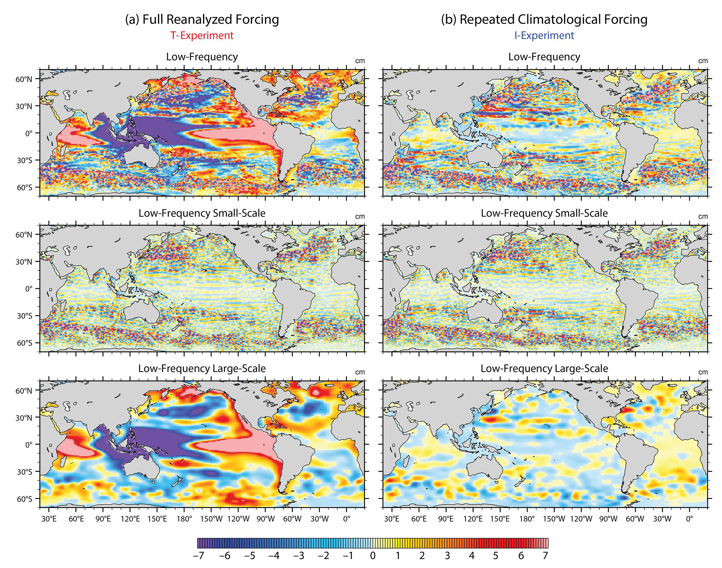
The left panels in Figure 1 present the November 1997 state of the LF sea level variability simulated by an “eddy-active” (1/12°, i.e., about 10 km resolution) global ocean model; this model was driven by full forcing², and therefore simulates variability that mimics the real ocean. Over this period, the prescribed atmospheric variability was characterized by the 1997–1998 El Niño event, which forced the strong, large-scale sea level response visible at low latitudes (bottom left). Smaller mesoscale eddies and fronts are superimposed on this large-scale signal almost everywhere in the global ocean (middle left).

 

Figure 1. Sea level anomaly in November 1997 in two NEMO (European Modelling of the Ocean) simulations at 1/12° resolution: one is driven by full forcing (a), the other by climatological forcing devoid of any interannual variability (b). All fields were low-pass filtered in time to remove periods shorter than 18 months. The top panel shows all spatial scales, the middle scales smaller than 6°, and the bottom scales larger than 12°. From Sérazin et al. (2015). > High res figure

 

The same model was then driven by climatological forcing³ devoid of any interannual and subannual frequencies, in order to isolate the LF CIV produced by the model. The right panels in Figure 1 show that despite the absence of any LF atmospheric variability, a strong LF CIV (upper) emerges, comprised of small mesoscale structures and zonally elongated “striations”⁴ (middle), and much larger-scale patterns (bottom). The sea level expression of LF CIV is comparable in amplitude with its fully forced counterpart in mid-latitude turbulent regions, in particular in the Antarctic Circumpolar Current (ACC), the Gulf Stream, and the Kuroshio, and their eastward extensions. This LF CIV is very weak in 2° resolution ocean models (Penduff et al., 2011; Grégorio et al., 2015), hence, presumably also in non-eddying CMIP-class AOGCMs. Its possible manifestations in AOGCMs resolving mesoscale turbulence are discussed in the last section.

The signature of LF CIV in realistic ocean models can be found in most oceanic variables and in various climate indices, including sea surface height (SSH; Penduff et al., 2011; Sérazin et al., 2015), sea surface temperature (SST; Sérazin, 2016), Atlantic meridional overturning circulation (AMOC) and heat transport (Grégorio et al., 2015), and large-scale transports above topography (Sgubin et al., 2014). But, does the LF CIV affect subsurface temperatures and OHC as well? In the following, we propose to disentangle the respective impacts of atmospheric variability and oceanic CIV on OHC at various depths, and discuss whether CIV may impact the detection and attribution of thermal signals in the ocean at various spatiotemporal scales.

LF ocean variability is strong and chaotic when isolated from LF forcing (i.e., under climatological forcing). Does it remain as chaotic when forced by a full reanalysis, or is it likely to be paced by the LF variability of the forcing? Can the CIV and the forced variability be disentangled, and what are their respective magnitudes? In the following, we describe the ensemble modeling approach that we designed to address these issues, and present the insight it provides about the forced and the chaotic OHC variabilities.

² In full forcing, the atmospheric variables used in the calculation of the ocean model surface boundary conditions are obtained from an atmospheric reanalysis. These atmospheric variables contain the full range of scales reconstructed by climate centers (ECMWF in the present case): from six-hourly to decadal timescales, and from a few degrees to global space scales.
³ Climatological forcing is derived from the mean annual cycle of the full atmospheric fields, and is repeatedly applied for several decades at the ocean model surface in order to isolate the oceanic LF CIV.
⁴ Altimeter observations confirm the existence of such non-stationary striations (https://www.aviso.altimetry.fr/fileadmin/documents/OSTST/2011/poster/​MultipleMigrating​Quasi-zonalJet-likeStructures_Melnichenko.pdf). See Chen et al. (2016), and the studies they discuss, for a review of these structures’ dynamics and their tight relation with mesoscale eddies.

 

A Large Ensemble of Global Ocean Simulations

We mentioned above that ensemble simulations allow climate modelers to simulate, then separate, the externally forced variability (due to, for example, GHGs) and the internally generated variability of the coupled ocean-atmosphere system. The OceaniC Chaos – ImPacts, strUcture, predicTability (OCCIPUT) project adopted an equivalent, but ocean-​focused, strategy to disentangle the externally forced ocean variability (due to atmospheric variability) and its internally generated variability (CIV). In practice, we perturbed the initial states of 50 global ocean/sea ice simulations that admit a portion of the turbulent regime (1/4° resolution), and forced them for 56 years (1960–2015) using the same full forcing⁵. Figure 4 in Bessières et al. (2017) shows, in two regions, the time series of the ensemble dispersion typical of a chaotic system: initial inter-member differences emerge at the mesoscale, grow exponentially during a few months (in strong CIV areas) or a few years (in weak CIV areas), then saturate and fluctuate around an equilibrium value. Such ensemble simulations produce time-varying ensemble probability density functions (ePDFs) of any given model variable (e.g., three-​dimensional temperature) or diagnostic quantity (e.g., OHC). Such ePDFs may be computed online to characterize the instantaneous spread among the ensemble members, or offline from post-​processed, larger-scale fields, such as temporal and/or spatial averages, or long-term OHC trends.

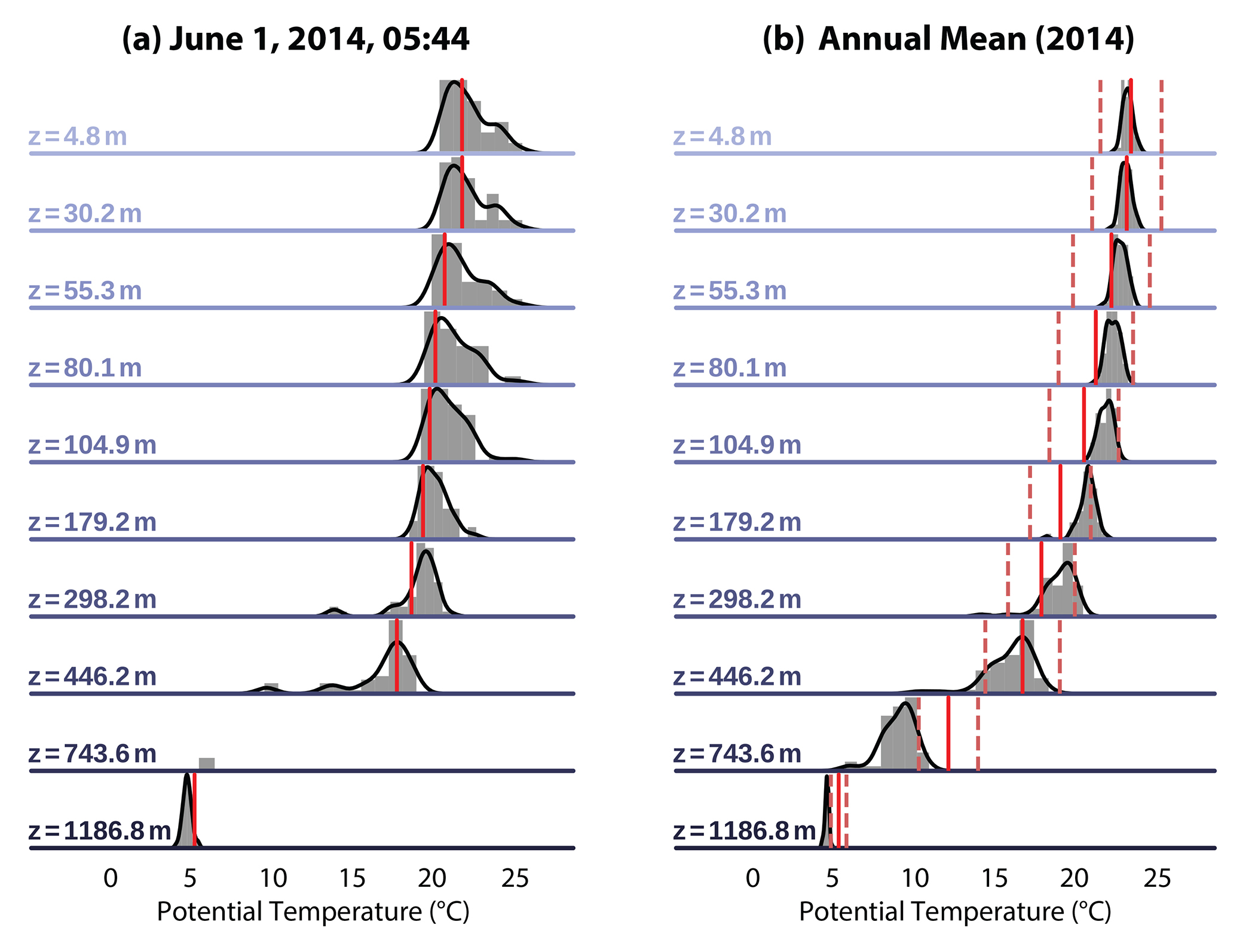
The left panel in Figure 2 shows the instantaneous ePDF of a temperature profile in the North Atlantic subtropics on June 1, 2014, built online from the 50 members, at the same location and instant as an Argo observation (red lines). The width of this instantaneous ePDF is about 5°C in the uppermost layers, reaches about 8°C at the thermocline depth (700–800 m), and is smaller below. The observed profile falls within the model ePDF at most depths, illustrating the model skill at this date and location. This model-derived ePDF represents the representativity uncertainty associated with the oceanic CIV for this particular profile.

 

Figure 2. Vertical profiles of temperature at 70°W, 36.2°N from various data sets. (a) Argo float observations on June 1, 2014 (red), and instantaneous ensemble probability density function (ePDF) in the OceaniC Chaos – ImPacts, strUcture, predicTability (OCCIPUT) ensemble at the same time and location (gray and black). (b) ePDFs of the 2014 annual-mean temperature in the OCCIPUT ensemble (gray and black), and Argo-based annual-mean temperature and associated uncertainty (red, ISAS annual climatology). > High res figure

 

The right panel in Figure 2 shows at the same location that the width of the ePDF of the annually averaged simulated temperature is also pronounced, in particular around the model thermocline depth⁶ where it is about 5°C. As expected indeed, the CIV has reached longer time scales during the 55 years of integration. In contrast to laminar ocean simulations where the variability is largely determined by the atmospheric variability, the CIV produced by high-resolution ocean models induces large thermal uncertainties, both instantaneously and at longer timescales.

Figure 2 illustrates the complexity of the CIV, with several non-Gaussian ePDF and hints of bimodality. Simple statistics can nevertheless provide interesting insight into model behavior: on the one hand, ensemble standard deviations (eSTDs) may be computed for any ePDF at any time, and these eSTDs can then be combined in time to estimate the CIV amplitude, or chaotic variability, σ_C. On the other hand, the temporal evolution of ensemble mean captures the variability that is shared by all members (driven by the same atmospheric variability): the temporal standard deviation of the ensemble mean provides an estimate of the forced variability, σ_F⁷. Forced and chaotic variabilities of OHC are now compared at various timescales.

⁵ The OCCIPUT project, the simulation strategy, and our ensemble version of the NEMO model are presented in Penduff et al. (2014), Bessières et al. (2017), and on https://meom-group.github.io/projects/occiput.
⁶ The upward decrease of the ensemble spread is an artifact of our forcing method; an alternative forcing technique yields a larger surface ensemble spread in temperature (see Bessières et al., 2017, page 1,101).
⁷ The detailed derivation of σ_C and σ_F is given in Leroux et al. (2018).

 

Forced and Chaotic Low-Frequency Variabilities of Ocean Heat Content

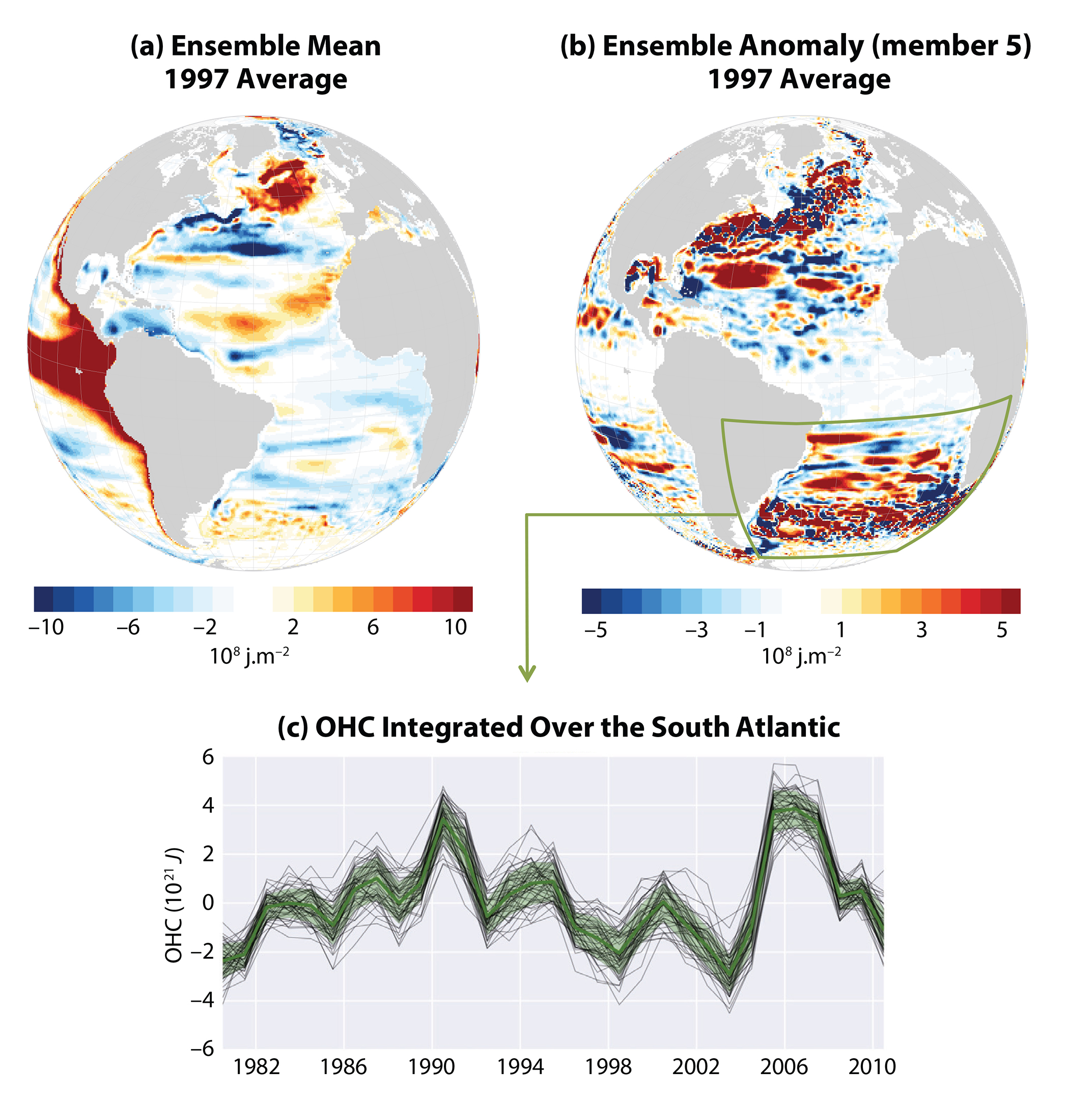
Figure 3a,b shows the forced and chaotic anomalies of the upper OHC (OHC_0–700m), averaged over 1997. The large 1997–1998 El Niño signal forced by the prescribed atmospheric winds has induced a large warming within all members in the eastern equatorial Pacific throughout 1997 (left panel). Superimposed on this forced response, each ensemble member generated a chaotic OHC_0–700m yearly anomaly (shown for member 5 in the right panel), with three key characteristics: (1) the phase of CIV in each member is different and independent of the atmosphere, despite the same forcing function; (2) while dominated by mesoscale eddies within the main currents, dominant LF CIV features can reach much larger scales (more than 1,000 km) in the subtropics; and (3) LF CIV features may exceed the amplitude of their forced counterparts, as in the large chaotic “warm pool” east of Florida generated by member 5 throughout 1997.

 

Figure 3. (a) Ensemble mean (forced part) and (b) ensemble anomaly (chaotic part in member 5) of the OHC0–700m yearly anomaly over 1997 (OHC = ocean heat content). (c) Evolution over 1980–2010 of yearly anomalies of OHC0-700m averaged over the South Atlantic, within the 50 OCCIPUT members (gray lines); the ensemble mean and ensemble standard deviation are shown in green. > High res figure

 

The chaotic low-frequency variability of OHC_0–700m remains substantial even at larger spatial scales. Figure 3c presents the time series of yearly OHC_0–700m integrated over the South Atlantic (10°–55°S) for each member. Despite the same atmospheric forcing applied over all members, yearly OHC_0–700m values may differ by up to 4.10²¹ J. This chaotic signal is about half of its forced counterpart (σ_C/σ_F = 0.5), which is large considering the size of the integration domain. This substantial CIV-related uncertainty should be kept in mind while interpreting modeled and observed time series.

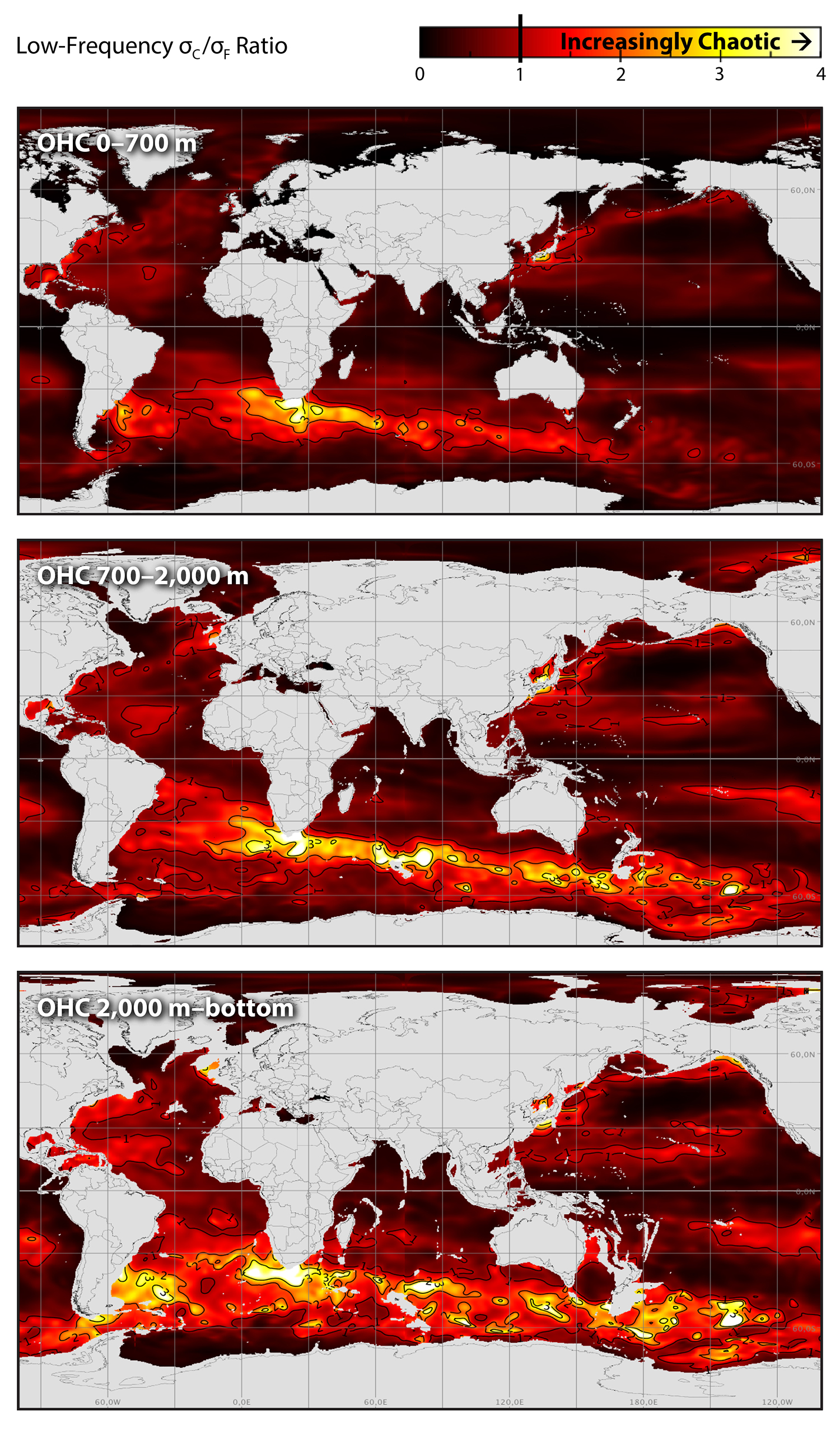
Figure 4 provides a global quantification of the ratio R = σ_C/σ_F over three depth ranges, restricted to the interannual-to-decadal (2–15 year timescales) variability of OHC at spatial scales larger than 1,000 km. Contours delineate regions where most of this LF variability is chaotic (i.e., where the atmospheric variability is a secondary driver of OHC fluctuations [R >1]). The largest R values in the Northern Hemisphere are found in the Kuroshio, the Gulf of Mexico, and the Gulf Stream; R also approaches unity in the central North Atlantic and in a coastal band linking Alaska to Japan. However, the absolute R maximum is located in the strongly eddying Agulhas retroflection: σ_C exceeds three times σ_F at all depths where the warm Indian waters flowing southwestward along Africa partly spill into the Atlantic as Agulhas rings, with the other part veering eastward and feeding the ACC’s Subtropical Front. This maximum is embedded within a much wider band that follows the ACC, where σ_C exceeds σ_F all the way from South America to the longitude of New Zealand in the upper layer.

 

Figure 4. Ratio R between the chaotic and the forced interannual-to-decadal variabilities (R = σC/σF) of the large-scale OHC (scales larger than 1,000 km): from top to bottom, layers 0–700 m, 700–2,000 m, and 2,000 m–bottom. All time scales longer than about 15 years (hence, the trends) were first removed from the 50-member yearly OHC fields in the three layers using the nonparametric LOcal regrESSion (LOESS) method. Adapted from Sérazin et al. (2017). > High res figure

 

Figure 4 also shows that areas where R >1 grow in size and number with increasing depth: below 2,000 m, σ_C exceeds σ_F all around Antarctica, with local maxima of R associated with topographic features. The subsurface LF OHC variability is also mostly chaotic in large areas along the equatorward flanks of the global ocean’s five subtropical gyres. This downward increase of R is certainly linked with a downward decrease in σ_F, because the atmospheric variability mostly impacts the surface. Preliminary investigations show that the LF chaotic OHC fluctuations are associated with two kinds of slow, random fluctuations at depth: vertical movements of density surfaces, and fluctuations of temperature along these surfaces.

Unlike these regional imprints of LF CIV, the evolution of the globally integrated OHC_0–700m index is almost the same among the 50 ensemble members. This illustrates the constraint exerted by the prescribed atmosphere on the simulated ocean variability at global scale: the CIV randomly advects heat anomalies at regional scales, with no significant impact on global OHC.

 

Detection and Attribution of Long-Term OHC Trends

Characteristic CIV timescales may, however, exceed the 2–15 year range considered above: a long (327-year) climatologically forced turbulent ocean simulation was shown to spontaneously generate CIV at periods reaching almost 100 years, with significant imprints on large-scale AMOC fluctuations (Grégorio et al., 2015) and on SSH trends in areas of strong eddy activity (Sérazin et al., 2016). Does this very low-frequency CIV influence OHC as well?

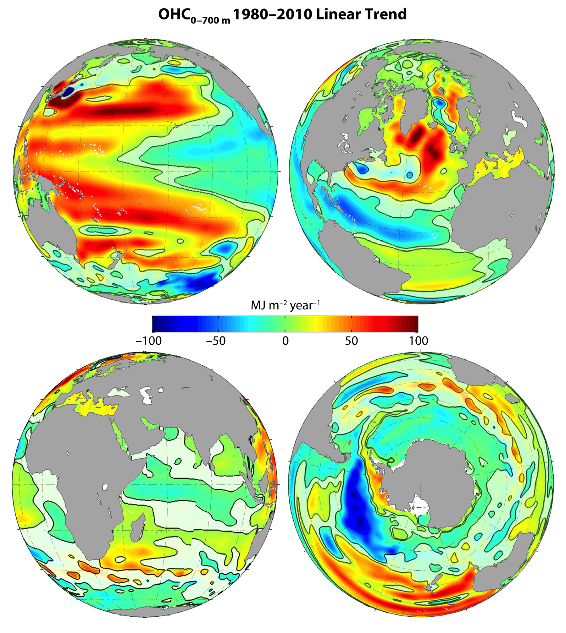
The fingerprint of multidecadal CIV can be detected by comparing the ensemble mean (forced part) and eSTD (CIV-induced part) of long-term OHC trends in the OCCIPUT ensemble. After subtracting the spurious model drift, Sérazin et al. (2017) derived these two statistics from 50 maps of large-scale, regional 31-year linear trends of OHC computed over the period 1980–2010. Figure 5 shows in color the forced trend of OHC_0–700m, masked by pale areas where it cannot be unambiguously attributed to the atmospheric evolution, including natural and anthropogenic trends. In these regions, OHC trends are rather random, due to the very low-frequency CIV. These regions are roughly located where the CIV was found to explain most of the 2–15 year OHC variability (Figure 4). The possible implications of these results for the monitoring and interpretation of the ocean heat content are discussed below.

 

Figure 5. Forced linear trend of OHC0–700m over 1980–2010 at scales larger than 1,000 km (colors) from four viewpoints. This forced trend is masked where it is smaller than twice the ensemble standard deviation. The spurious model trend was estimated from a climatological simulation and removed beforehand. Adapted from Sérazin et al. (2017). > High res figure

 

Implications and Outlook

Ocean simulations driven by both full and climatological reanalysis-based atmospheric forcings show that, when mesoscale turbulence is (even partly) resolved, a strong LF variability spontaneously emerges from the ocean. This chaotic intrinsic ocean variability is largest at mid-latitudes, affects multiple fields, and reaches large spatiotemporal scales. The OCCIPUT ensemble was designed to disentangle intrinsic and atmospherically forced variabilities, and assess their impacts on climate-relevant oceanic indices. Results show that the intrinsic variability remains chaotic (hence the CIV acronym) under realistic forcing, is able to compete with, and even dominate, the forced variability in many regions. It has a strong fingerprint on OHC at all depths, up to multidecadal and gyre scales. As with any simulation, these model results may be partly biased and should be interpreted with care. Nevertheless, they have various implications. In the following we discuss those concerning the detection and attribution of observed signals, and comment on the role of the turbulent ocean in the climate system.

Figure 2 illustrates an interesting paradigm (articulated by Holloway, 2004): we may consider that any individual in situ or satellite measurement samples the oceanic state that was randomly picked by nature from an ensemble of possibilities. The OCCIPUT simulation describes these possibilities. If the model has skill, then instantaneous ePDFs (e.g., Figure 2a) can provide information about the imprint of multiscale oceanic “chaos” on each observation: the wider the ePDF, the stronger this imprint, and the less the observation is representative of the forced component of the ocean state. This information could be used, for example, to weight individual hydrographic profiles when building gridded products from observations; spatiotemporal variances are sometimes used to estimate these weights, but ePDFs may be better adapted for this purpose because they are available at each location and time. Simulated equivalents of all hydrographic profiles contained in the EN4 database (Good et al., 2013) were extracted online from the 50 members during the OCCIPUT simulation. Each set of these “ensemble synthetic observations” is associated with an observed T/S profile: it can be used to address the issues mentioned above, and to probabilistically evaluate the simulation.

These results suggest that the observed evolution of regional temperatures (e.g., from Argo or CTD data) should be interpreted carefully. In certain regions (see Figures 4 and 5), the interannual-to-decadal variability and 30-year trends of regional temperatures could be mostly due to the CIV, whose phase is random and uncorrelated with that of the atmospheric variability. Figure 5 suggests that a 30-year trend measured south of Australia, for instance, should not be readily attributed to atmospheric or anthropogenic causes, but may instead have a random sign. This uncertainty exists regardless of the measurement error; it depends on the ocean dynamics. Such an ensemble could help reassess the detection and attribution criteria for observed trends and fluctuations (e.g., see Barnett et al., 2001), in the presence of mesoscale turbulence. Efforts are currently underway to evaluate the impact of LF CIV on the warming hiatus in the past decades, and to try to attenuate the CIV signal in observed time series.

Prescribing the atmospheric forcing of the ensemble simulation was necessary to separate the forced and the chaotic oceanic LF variabilities, and to answer the questions above, but what might the results presented here imply for the other components of the climate system? Because multidecadal ocean thermal variability tends to drive the atmosphere (e.g., Gulev et al. 2013), and because the largest chaotic LF OHC signals are found where air-sea heat fluxes are largest in nature, the atmosphere will very likely be influenced by oceanic LF CIV in an AOGCM that resolves the mesoscale. Further work is needed to assess whether new atmospheric or coupled LF variability modes will also emerge in high-resolution coupled models, or whether the predictability of these modes will be affected by CIV.

Oceanic CIV also yields local differences in sea ice concentration, thickness, and velocity in the marginal ice zone among the OCCIPUT members. These differences yield distinct air-sea fluxes and convective activities in polar regions, which are in turn able to increase the ensemble spread in subsurface temperatures. The hemispheric integrals of sea ice volume are, however, almost identical among the members (see discussion in Griffies et al., 2009). Finally, recent simulations indicate that the physical CIV induces a substantial low-frequency variability in the marine biogeochemistry, with geographical distributions and magnitudes dependent on the tracer considered. The oceanic CIV may have further impact on other climate system components, such as ice shelves or the hydrological cycle. Investigations of these possible consequences are left for the future.

The robustness of these results will have to be confirmed in other models at different resolutions. However, they demonstrate that low-frequency oceanic variability in the presence of mesoscale turbulence is no longer a slave to the atmosphere or solely due to air-sea coupling: part of it emerges spontaneously with a chaotic behavior, impacting many oceanic fields, and the ocean heat content in particular. The implications of these results for the detection and attribution of climate signals in the warming ocean need to be assessed in more detail.

Penduff, T., G. Sérazin, S. Leroux, S. Close, J.-M. Molines, B. Barnier, L. Bessières, L. Terray, and G. Maze. 2018. Chaotic variability of ocean heat content: Climate-relevant features and observational implications. Oceanography 31(2):63–71, https://doi.org/10.5670/oceanog.2018.210.

Arbic, B.K., M. Müller, J.G. Richman, J.F. Shriver, A.J. Morten, R.B. Scott, G. Sérazin, and T. Penduff. 2014. Geostrophic turbulence in the frequency–​wavenumber domain: Eddy-driven low-frequency variability. Journal of Physical Oceanography 44:2,050–2,069, https://doi.org/​10.1175/JPO-D-13-054.1.
1. Arbic, B.K., R.B. Scott, G.R. Flierl, A.J. Morten, J.G. Richman, and J.F. Shriver. 2012. Nonlinear cascades of surface oceanic geostrophic kinetic energy in the frequency domain. Journal of Physical Oceanography 42:1,577–1,600, https://doi.org/​10.1175/JPO-D-11-0151.1.
2. Barnett, T.P., D.W. Pierce, and R. Schnur. 2001. Detection of anthropogenic climate change in the world’s oceans. Science 292:270–274, https://doi.org/​10.1126/science.1058304.
3. Barnier, B., T. Penduff, and C. Langlais. 2010. Eddying vs. laminar ocean circulation models and their applications. Chapter 10 in Operational Oceanography in the 21st Century. A. Schiller and G.B. Brassington, eds, Springer.
4. Bellomo, K., L.N. Murphy, M.A. Cane, A.C. Clement, and L.M. Polvani. 2017. Historical forcings as main drivers of Atlantic multidecadal variability in the CESM Large Ensemble. Climate Dynamics 50:3,687–3,698, https://doi.org/10.1007/s00382-017-3834-3.
5. Bessières, L., S. Leroux, J.-M. Brankart, J.-M. Molines, M.-P. Moine, P.-A. Bouttier, T. Penduff, L. Terray, B. Barnier, and G. Sérazin. 2017. Development of a probabilistic ocean modelling system based on NEMO 3.5: Application at eddying resolution. Geoscientific Model Development 10:1,091–1,106, https://doi.org/10.5194/gmd-10-1091-2017.
6. Charney, J.G. 1971. Geostrophic turbulence. Journal of Atmospheric Sciences 28:1,087–1,095, https://doi.org/10.1175/​1520-0469(1971)028​<1087:GT>​2.0.CO;2.
7. Chen, C., I. Kamenkovich, and P. Berloff. 2016. Eddy trains and striations in quasigeostrophic simulations and the ocean. Journal of Physical Oceanography 46:2,807–2,825, https://doi.org/​10.1175/JPO-D-16-0066.1.
8. Church, J.A., N.J. White, L.F. Konikow, C.M. Domingues, J.G. Cogley, E. Rignot, J.M. Gregory, M.R. van den Broeke, A.J. Monaghan, and I. Velicogna. 2011. Revisiting the Earth’s sea-level and energy budgets from 1961 to 2008. Geophysical Research Letters 38, L18601, https://doi.org/​10.1029/​2011GL048794.
9. Colin de Verdière, A., and T. Huck. 1999. Baroclinic instability: An oceanic wavemaker for interdecadal variability. Journal of Physical Oceanography 29:893–910, https://doi.org/​10.1175/​1520-0485​(1999)029​<0893:BIAOWF>​2.0.CO;2.
10. Ferrari, R., and C. Wunsch. 2009. Ocean circulation kinetic energy: Reservoirs, sources, and sinks. Annual Review of Fluid Mechanics 41:253–282, https://doi.org/10.1146/annurev.fluid.40.111406.102139.
11. Fjortoft, R. 1953. On the changes in the spectral distribution of kinetic energy for two-dimensional nondivergent flow. Tellus 5:225–230, https://doi.org/​10.3402/tellusa.v5i3.8647.
12. Gleckler, P.J., B.D. Santer, C.M. Domingues, D.W. Pierce, T.P. Barnett, J.A. Church, K.E. Taylor, K.M. AchutaRao, T.P. Boyer, M. Ishii, and P.M. Caldwell. 2012. Human-induced global ocean warming on multidecadal timescales. Nature Climate Change 2:524–529, https://doi.org/​10.1038/nclimate1553.
13. Good, S.A., M.J. Martin, and N.A. Rayner. 2013. EN4: Quality controlled ocean temperature and salinity profiles and monthly objective analyses with uncertainty estimates. Journal of Geophysical Research 118:6,704–6,716, https://doi.org/​10.1002/​2013JC009067.
14. Grégorio, S., T. Penduff, G. Sérazin, J.-M. Molines, B. Barnier, and J. Hirschi. 2015. Intrinsic variability of the Atlantic Meridional Overturning Circulation at interannual-to-multidecadal timescales. Journal of Physical Oceanography 45(7):1,929–1,946, https://doi.org/10.1175/JPO-D-14-0163.1.
15. Gulev, S.K., M. Latif, N. Keenlyside, W. Park, and K.P. Koltermann. 2013. North Atlantic Ocean control on surface heat flux on multidecadal timescales. Nature 499:464–467, https://doi.org/10.1038/nature12268.
16. Griffies, S.M., A. Biastoch, C. Böning, F. Bryan, G. Danabasoglu, E.P. Chassignet, M.H. England, R. Gerdes, H. Haak, R.W. Hallberg, and others. 2009. Coordinated ocean-ice reference experiments (COREs). Ocean Modelling 26(1):1-46, https://doi.org/10.1016/j.ocemod.2008.08.007.
17. Holloway, G. 2004. From classical to statistical ocean dynamics. Surveys in Geophysics 25:203–219, https://doi.org/10.1007/s10712-004-1272-3.
18. Huck, T., O. Arzel, and F. Sévellec. 2015. Multidecadal variability of the overturning circulation in presence of eddy turbulence. Journal of Physical Oceanography 45(1):157–173, https://doi.org/​10.1175/JPO-D-14-0114.1.
19. IPCC. 2013. Climate Change, 2013: The Physical Science Basis. Contribution of Working Group I to the Fifth Assessment Report of the Intergovernmental Panel on Climate Change. T.F. Stocker, D. Qin, G.-K. Plattner, M. Tignor, S.K. Allen, J. Boschung, A. Nauels, Y. Xia, V. Bex, and P.M. Midgley, eds, Cambridge University Press, Cambridge, UK, and New York, NY, USA, 1,535 pp., https://doi.org/10.1017/CBO9781107415324.
20. Kraichnan, R.H. 1967. Inertial ranges in two-dimensional turbulence. Physics of Fluids 10:1,417–1,423, https://doi.org/10.1063/1.1762301.
21. Leroux, S., T. Penduff, L. Bessières, J. Molines, J. Brankart, G. Sérazin, B. Barnier, and L. Terray. 2018. Intrinsic and atmospherically forced variability of the AMOC: Insights from a large-ensemble ocean hindcast. Journal of Climate 31:1,183–1,203, https://doi.org/10.1175/JCLI-D-17-0168.1.
22. Llovel, W., S. Guinehut, and A. Cazenave. 2010. Regional and interannual variability in sea level over 2002–2009 based on satellite altimetry, Argo float data and GRACE ocean mass. Ocean Dynamics 60:1,193–1,204, https://doi.org/10.1007/s10236-010-0324-0.
23. Menary, M.B., W. Park, K. Lohmann, M. Vellinga, M.D. Palmer, M. Latif, and J.H. Jungclaus. 2012. A multimodel comparison of centennial Atlantic meridional overturning circulation variability. Climate Dynamics 38:2,377–2,388, https://doi.org/​10.1007/s00382-011-1172-4.
24. Nerem, R.S., B.D. Beckley, J.T. Fasullo, B.D. Hamlington, D. Masters, and G.T. Mitchum. 2018. Climate-change-driven accelerated sea-level rise detected in the altimeter era. Proceedings of the National Academy of Sciences of the United States of America 115(9):2,022–2,025, https://doi.org/​10.1073/pnas.1717312115.
25. O’Kane, T.J., R.J. Matear, M.A. Chamberlain, J.S. Risbey, B.M. Sloyan, and I. Horenko. 2013. Decadal variability in an OGCM Southern Ocean: Intrinsic modes, forced modes and metastable states. Ocean Modelling 69:1–21, https://doi.org/​10.1016/j.ocemod.2013.04.009.
26. O’Rourke, A.K., B.K. Arbic, and S.M. Griffies. 2018. Frequency-domain analysis of atmospherically forced versus intrinsic ocean surface kinetic energy variability in GFDL’s CM2-O model hierarchy. Journal of Climate 31:1,789–1,810, https://doi.org/​10.1175/JCLI-D-17-0024.1.
27. Penduff, T., B. Barnier, L. Terray, L. Bessières, G. Sérazin, J.-M. Brankart, M.-P. Moine, J.-M. Molines, and P. Brasseur. 2014. Ensembles of eddying ocean simulations for climate. CLIVAR Exchanges No. 65 19(2):26–29.
28. Penduff, T., M. Juza, B. Barnier, J. Zika, W.K. Dewar, A.-M. Treguier, J.-M. Molines, and N. Audiffren. 2011. Sea-level expression of intrinsic and forced ocean variabilities at interannual time scales. Journal of Climate 24:5,652–5,670, https://doi.org/10.1175/JCLI-D-11-00077.1.
29. Purkey, S.G., and G.C. Johnson. 2010. Warming of global abyssal and deep Southern Ocean waters between the 1990s and 2000s: Contributions to global heat and sea level rise budgets. Journal of Climate 23:6,336–6,351, https://doi.org/​10.1175/​2010JCLI3682.1.
30. Rhein, M., S.R. Rintoul, S. Aoki, E. Campos, D. Chambers, R.A. Feely, S. Gulev, G.C. Johnson, S.A. Josey, A. Kostianoy, and others. 2013. Observations: Ocean. Chapter 3 in Climate Change 2013: The Physical Science Basis. Contribution of Working Group I to the Fifth Assessment Report of the Intergovernmental Panel on Climate Change, T.F. Stocker, D. Qin, G.-K. Plattner, M. Tignor, S.K. Allen, J. Boschung, A. Nauels, Y. Xia, V. Bex, and P.M. Midgley, eds, Cambridge University Press, Cambridge, UK, and New York, NY, USA.
31. Riser S.C., H.J. Freeland, D. Roemmich, S. Wijffels, A. Troisi, M. Belbéoch, D. Gilbert, J. Xu, S. Pouliquen, A. Thresher, and others. 2016. Fifteen years of ocean observations with the global Argo array. Nature Climate Change 6:145–153, https://doi.org/10.1038/nclimate2872.
32. Scott, R.B., and F. Wang. 2005. Direct evidence of an oceanic inverse kinetic energy cascade from satellite altimetry. Journal of Physical Oceanography 35:1,650–1,666, https://doi.org/​10.1175/JPO2771.1.
33. Sérazin, G. 2016. Empreinte de la variabilité intrinsèque océanique sur l’océan de surface: caractérisation et processus. PhD Thesis, Université de Toulouse.
34. Sérazin, G., A. Jaymond, S. Leroux, T. Penduff, L. Bessières, W. Llovel, B. Barnier, J.-M. Molines, and L. Terray. 2017. A global probabilistic study of the ocean heat content low-frequency variability: Atmospheric forcing versus oceanic chaos. Geophysical Research Letters 44:5,580–5,589, https://doi.org/10.1002/2017GL073026.
35. Sérazin, G., B. Meyssignac, T. Penduff, L. Terray, B. Barnier, and J.-M. Molines. 2016. Quantifying uncertainties on regional sea-level rise induced by multi-decadal oceanic intrinsic variability. Geophysical Research Letters 43:8,151–8,159, https://doi.org/10.1002/2016GL069273.
36. Sérazin, G., T. Penduff, B. Barnier, J.M. Molines, B.K. Arbic, M. Müller, and L. Terray. In press. Inverse cascades of kinetic energy as a source of low-​frequency intrinsic variability: A global OGCM study. Journal of Physical Oceanography, https://doi.org/​10.1175/​JPO-D-17-0136.1.
37. Sérazin, G., T. Penduff, S. Grégorio, B. Barnier, J.-M. Molines, and L. Terray. 2015. Intrinsic variability of sea-level from global 1/12° ocean simulations: Spatio-temporal scales. Journal of Climate 28:4,279–4,292, https://doi.org/​10.1175/JCLI-D-14-00554.1.
38. Sévellec, F., and A.V. Fedorov. 2013. The leading, interdecadal eigenmode of the Atlantic meridional overturning circulation in a realistic ocean model. Journal of Climate 26:2,160–2,183, https://doi.org/​10.1175/JCLI-D-11-00023.1.
39. Sgubin, G., S. Pierini, and H.A. Dijkstra. 2014. Intrinsic variability of the Antarctic Circumpolar Current system: Low-and high-frequency fluctuations of the Argentine Basin flow. Ocean Science 10:201–213, https://doi.org/10.5194/os-10-201-2014.
40. Taylor, K.E., R.J. Stouffer, and G.A. Meehl. 2012. An overview of CMIP5 and the experiment design. Bulletin of the American Meteorological Society 93:485–498, https://doi.org/10.1175/BAMS-D-11-00094.1.
41. Venaille, A., J. Le Sommer, J.-M. Molines, and B. Barnier. 2011. Stochastic variability of oceanic flows above topography anomalies. Geophysical Research Letters 38, L16611, https://doi.org/​10.1029/​2011GL048401.
42. Wolfe, C.L., P. Cessi, and B.D. Cornuelle. 2017. An intrinsic mode of interannual variability in the Indian Ocean. Journal of Physical Oceanography 47:701–719, https://doi.org/10.1175/JPO-D-16-0177.1.
43. Zivkovic, T., and K. Rypdal. 2013. ENSO dynamics: Low-dimensional-chaotic or stochastic? Journal of Geophysical Research 118:2,161–2,168, https://doi.org/​10.1002/jgrd.50190.

This is an open access article made available under the terms of the Creative Commons Attribution 4.0 International License (https://creativecommons.org/licenses/by/4.0/), which permits use, sharing, adaptation, distribution, and reproduction in any medium or format as long as users cite the materials appropriately, provide a link to the Creative Commons license, and indicate the changes that were made to the original content. Images, animations, videos, or other third-party material used in articles are included in the Creative Commons license unless indicated otherwise in a credit line to the material. If the material is not included in the article’s Creative Commons license, users will need to obtain permission directly from the license holder to reproduce the material.