Introduction
Some of the most energetic motions in the upper ocean are mesoscale eddies and wind-driven internal waves (e.g., Ferrari and Wunsch, 2010, and references therein). The latter tend to have frequencies close to the inertial frequency, f = 2Ωsinλ (where Ω is Earth’s angular velocity and λ is latitude) and are known as near-inertial waves (NIWs). The dynamics of NIWs are controlled by Earth’s rotation through the Coriolis force, but variations in the net spin of fluid caused by vertical vorticity, ζ, of a current, for example, associated with the swirl of a mesoscale eddy, can greatly modify properties of NIWs. This effect is quantified by the effective inertial frequency fe f f ≈ f + ζ/2, which is lower in anticyclones and higher in cyclones (Kunze, 1985). NIWs can therefore oscillate at lower frequencies within an anticyclone and thus lag NIWs outside of the eddy where fe f f is higher. This detuning implies that wind-driven NIWs are focused into anticyclones and downward out of the mixed layer into the pycnocline. Observational evidence of this phenomenon has been documented from the 1980s (e.g., Kunze and Sanford, 1984; Kunze, 1986) up to the present day (see Essink et al., 2022, for a particularly compelling example in a Kuroshio anticyclonic eddy). The phenomenon was coined the inertial chimney effect by Lee and Niiler (1998) but has recently been renamed the inertial drainpipe effect by Asselin and Young (2020) to more accurately evoke the image of downward energy propagation in anticyclones.
The preferential flux of NIW energy into anticyclones implies that there must be energy loss mechanisms within the eddies to maintain equilibrium. Several possible energy sinks are schematized in Figure 1. As surface-forced NIWs propagate downward in weakening anticyclonic vorticity, they encounter a critical layer where their vertical wavelengths and group velocities shrink so that they stall and amplify (Kunze, 1985, 1986). Microstructure observations supporting loss of NIW energy to turbulent dissipative sinks in critical layers have been reported at the bases of Gulf Stream warm-core rings (Lueck and Osborn, 1986; Kunze et al., 1995) and toward the bottoms of anticyclones in the Mediterranean, Arctic, and Norwegian Seas (Cuypers et al., 2012; Kawaguchi et al., 2016; Fer et al., 2018). The mechanism could be widespread and might contribute to seasonal variations in mixing in the thermocline (Whalen et al., 2018).
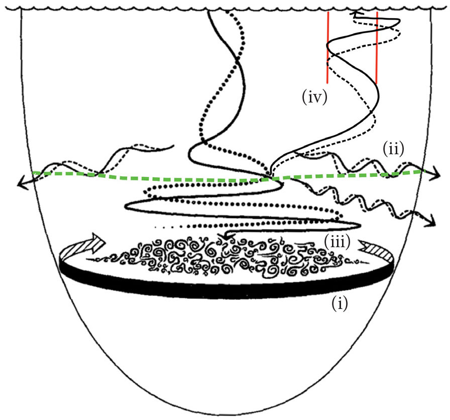
FIGURE 1. Schematic illustrating four hypothesized sinks of near-inertial wave (NIW) energy trapped in an anticyclone (adapted from Kunze et al., 1995; © American Meteorological Society. Used with permission). A downward-propagating NIW focused in the center of an anticyclone via the inertial drainpipe effect has an east (solid line) and north (dotted line) velocity 90° out of phase that causes the velocity vector to spiral clockwise with depth. As the wave approaches the depth where its frequency is equal to fe f f ≈ f + ζ/2 (critical layer), its vertical wavelength and propagation speed shrink. Its energy increases until it is lost to either (i) the mean circulation, (ii) untrapped, higher-frequency internal waves, or (iii) turbulence. If the anticyclone has a jump in stratification (dashed green line), part of the NIW energy is reflected off the jump, partially blocking the inertial drainpipe (iv) with a velocity vector that spirals counterclockwise with depth. Submesoscale filaments with anticyclonic vorticity (red lines) on the edge of the eddy can focus the upward-propagating NIW in an inertial chimney, leading to wave amplification, breaking, and dissipation near the surface. > High res figure
|
Apart from losing energy to turbulence, NIWs in critical layers can transfer energy to an anticyclone via wave-mean flow interactions (Figure 1i) or to higher-frequency internal waves through wave-wave interactions (Kunze et al., 1995). These higher-frequency waves are not necessarily bound to the anticyclone and could radiate energy away from the eddy (Figure 1ii).
In this article, we describe a fourth sink for NIWs in an inertial drainpipe. It involves the partial reflection of downward-propagating NIWs off the jump in stratification that can be found near the base of an anticyclone and subsequent dissipation of the resulting upward-propagating NIWs near the surface (Figure 1iv). Evidence for this energy pathway comes from observations of NIWs and turbulence on the edge of an anticyclone in the Iceland Basin, which are described below and interpreted using theory and idealized numerical simulations.
Overview of Observations
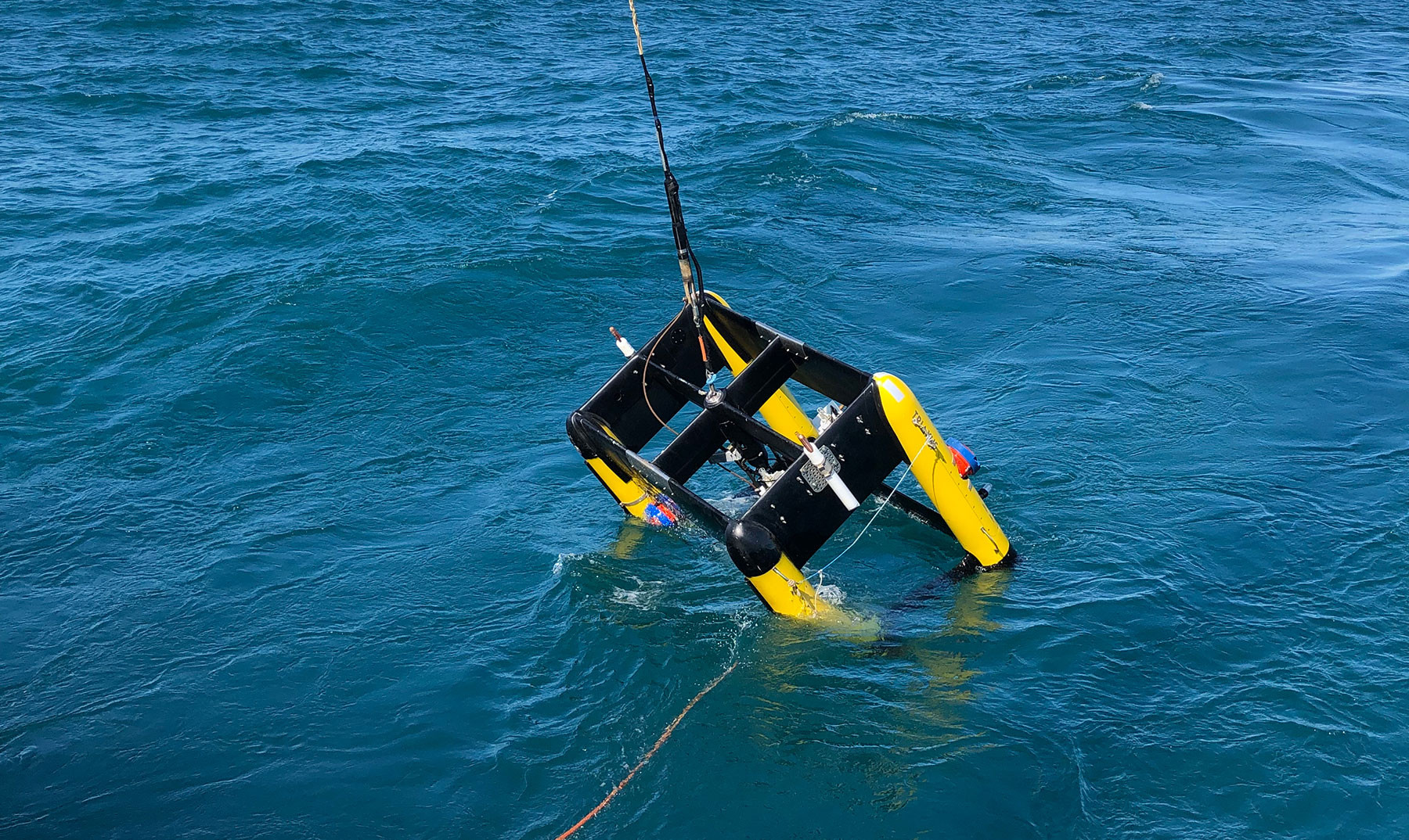
The measurements were made in the Iceland Basin as part of the Near-Inertial Shear and Kinetic Energy in the North Atlantic experiment (NISKINe), whose goal was to study NIWs in the Iceland Basin from wind generation to turbulent dissipation, including their interactions with the mesoscale and submesoscale eddy field. The observations presented here are from the ”Fence Survey” conducted June 9–12, 2019, from R/V Neil Armstrong. The survey followed an array of drifting assets including EM-APEX floats (e.g., Girton et al., 2024, in this issue) that were deployed toward the outer edge of an anticyclone. The focus of this article will be on observations made from the ship as it transected the eddy’s rim while traveling downstream with the array of drifting assets. These include measurements of velocity from 150 kHz and 300 kHz ship-mounted acoustic Doppler current profilers (ADCPs) in the upper 400 m and 100 m, with bin size of 8 m and 2 m, respectively, processed using UHDAS (https://currents.soest.hawaii.edu/). Hydrography was collected using a Triaxus-towed, undulating profiler. Triaxus profiled from the sea surface to 170 m depth at vertical speeds of 0.8–1.0 m s−1 and tow speeds of 2–4 m s−1. The profiler carried an extensive payload of physical and bio-optical sensors, including a Sea-Bird SBE 9plus CTD equipped with dual, pumped temperature (SBE 3plus) and conductivity (SBE 4C) sensors sampled at 24 Hz. Hydrography from the Triaxus CTD was augmented by six full-depth casts with the ship’s Sea-Bird TSG CTD along a line that transected the anticyclone June 8–9, 2019 (Figure 2a). A GusT probe (Becherer et al., 2020) attached to Triaxus (see article title page) was used to measure temperature microstructure of flow undisturbed by the instrument package and from which turbulence diffusivity (KT) and the dissipation rate of turbulence kinetic energy (ε) were estimated. The GusT probe is a miniaturized version of a χpod (Moum and Nash, 2009), which has now seen extensive use on oceanographic moorings (Moum et al., 2023). Implementations of χpods to date have been on fixed platforms where the fluid moves past the sensor. In this implementation, the sensor moves through the fluid. Spectral fits in the inertial-convective subrange (Zhang and Moum, 2010) were used to infer estimates of KT and ε.
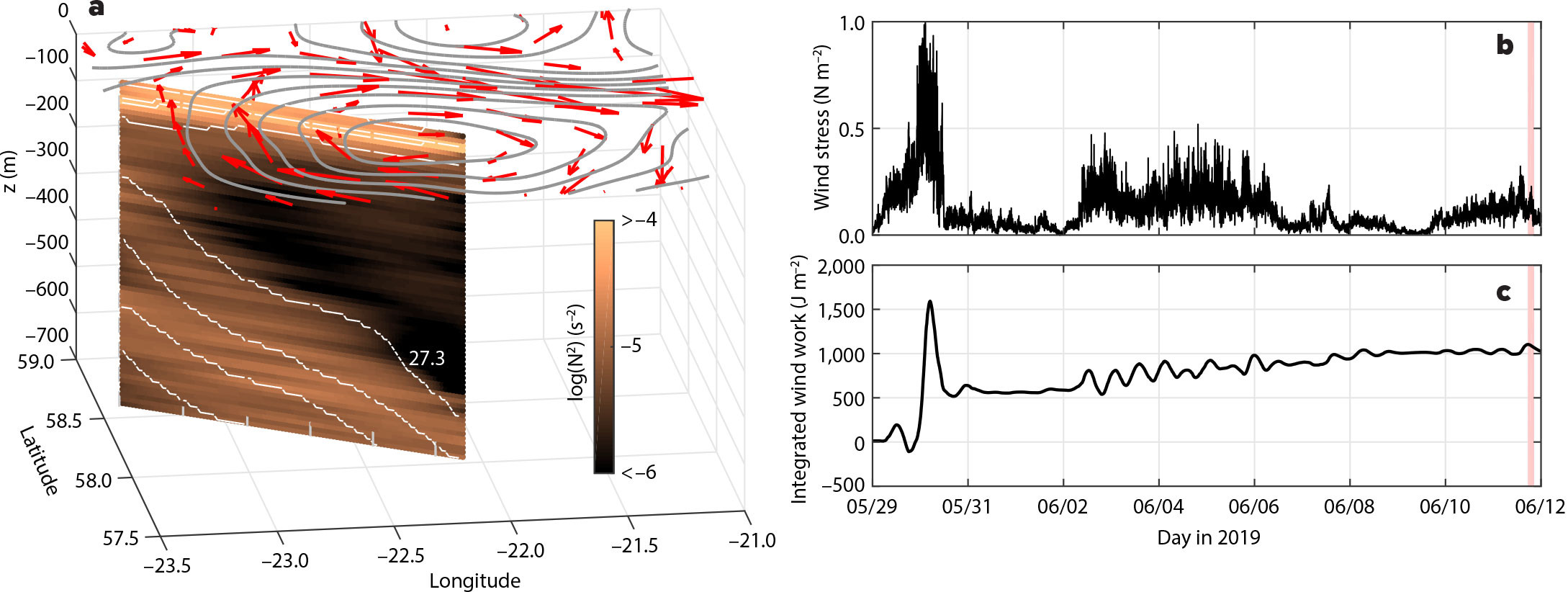
FIGURE 2. Structure of the anticyclone that is the focus of this study and the wind-forcing during the field campaign. (a) The sea-surface height anomaly (from AVISO, gray contours), surface velocity (red vectors), potential density field (contoured in white every 0.1 kg m–3), and N2 (shading) in the anticyclone. The section of potential density was mapped using hydrography from six deep CTD casts taken at the locations indicated by the gray tick marks at the bottom of the transect. Time series of (b) wind-stress observed from the ship during the cruise and (c) kinetic energy input to near-inertial motions by the winds estimated using a slab mixed-layer model. The vertical red lines in (b) and (c) indicate the time when the section with upward-propagating NIWs was collected (Figure 4b). > High res figure
|
Anticyclone and Wind Forcing
The background flow in the study region is characterized by an anticyclone with maximum velocities ~0.5 m s−1 and radius ~75 km. The core of the anticyclone is filled with remnant winter water and weak stratification. More specifically, the square of the buoyancy frequency, N2 = –g/ρ0∂σt/∂z (where g is the acceleration due to gravity, ρ0 a reference density equal to 1,000 kg m–3, σt the potential density, and z is the vertical coordinate), in these waters can be less than 1 × 10⁻⁶ s–2 (Figure 2a). The winter water is bounded above and below by more stratified waters. At the base of the winter water layer is an abrupt 40-fold increase in N2 crossing into the permanent pycnocline. The winter water layer is also capped by a seasonal pycnocline between 10 and 60 m. In the seasonal pycnocline, N2 can exceed 1 × 10⁻⁴ s–2 (Figure 2a). A ~10 m thick mixed layer tops all three of these layers.
The permanent pycnocline has a bowl-like shape in the anticyclone, rising from a depth of 700 m in the eddy center to 400 m at its edge (Figure 2a). The corresponding tilt in the pycnocline results in a surface-intensified anticyclonic circulation. However, vertical gradients in the circulation are mostly confined to the depths of the permanent pycnocline (i.e., between 500 and 1,000 m) such that, within the winter water layer, the anticyclonic circulation is fairly barotropic on the larger scale of the eddy.
The Fence Survey revealed that the anticyclone also has finer-scale filamentary features near its rim. Here, filaments less than 5 km wide and ~40 km long were evident in both salinity and vertical vorticity (Figure 3). Vertical vorticity was approximated as ζ = ∂val/∂xcs, where val is the along-stream component of the flow on each section and xcs is a cross-stream coordinate defined to be perpendicular to the maximum depth-averaged flow on the section and increasing toward the center of the eddy. Vertical vorticity covaries with salinity, with cyclonic vorticity tending to coincide with fresher waters, while the filaments of saltier water are correlated with stronger anticyclonic vorticity (Figure 3). Saline filaments do not reach the surface but are capped by the seasonal pycnocline. Anticyclonic vorticity in the filaments is also weaker near the surface (Figure 3d), which has important implications for the propagation of NIWs, as will be discussed in the next section.
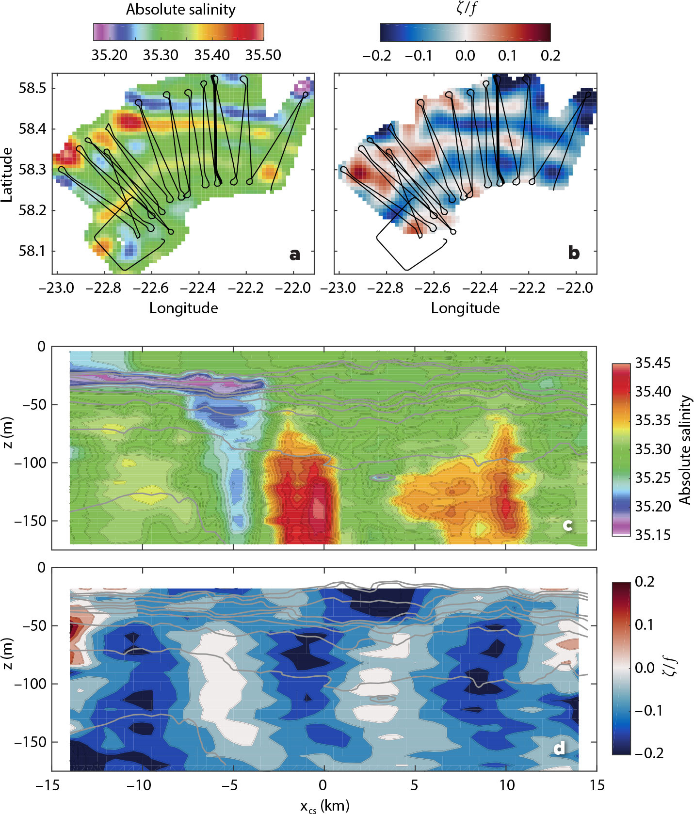
FIGURE 3. Filamentary nature of salinity (a,c) and vorticity (b,d) fields observed on the Fence Survey along the northern rim of the anticyclone (ship track in black). Mapped plan-view sections at z = –100 m of (a) absolute salinity and (b) vertical vorticity normalized by f. Vertical sections of absolute salinity (c) and vertical vorticity normalized by f (d) along the transect indicated by the thick black lines in (a) and (b). Potential density is contoured in gray every 0.05 kg m–3 in (c) and (d). This is the same transect where the upward-propagating NIWs were observed (Figure 4b). xcs unconventionally increases towards the center of the eddy. > High res figure
|
Winds during the field campaign were conducive to generating NIWs. The strongest wind event occurred during the passage of a storm on May 30, yielding a wind-stress that approached 1 N m–2 (Figure 2b). After the storm, before and during the Fence Survey (starting on June 9), the winds were weaker and steadier, so less prone to creating NIWs. To quantify how effective the winds were at generating NIWs, an estimate for the amount of kinetic energy injected into near-inertial motions was calculated using a slab mixed-layer model forced by the observed winds and assuming a mixed-layer depth of 10 m, a value representative of what was observed during the cruise (Pollard and Millard, 1970). The model integrates the linear momentum equations averaged over the mixed layer and uses Rayleigh damping with a damping coefficient of 0.1 f. Velocity from the model and wind stress were used to estimate the time-integrated wind work, a measure of the kinetic energy input to near-inertial motions by winds. The model indicates that the largest and most abrupt injection of kinetic energy by the winds occurs during the May 30 wind event (Figure 2c), suggesting that the storm was an effective NIW generator. Surveys on the southwest edge of the anticyclone (near 57°48'N, 23°30'W) made within a few days of the storm revealed acceleration of near-inertial motions in the mixed layer and seasonal pycnocline, as well as their subsequent decay through downward radiation of NIWs into the anticyclone (Thomas et al., 2020, 2023, and 2024, in this issue).
Evidence of Upward-Propagating NIWs and a True Inertial Chimney
Banded patterns in vertical shear, a signature of NIWs, were observed on several of the sections of the Fence Survey. The shear bands were angled down toward the center of the anticyclone (Figure 4b). The section was completed in a fraction of an inertial period, Ti = 14 hours, (i.e., 0.18Ti or 2.5 hours). Therefore, the shear can be interpreted as a snapshot of a NIW beam. The tilt in the shear bands indicates possible directions of wave energy propagation, either down and toward the center of the eddy, or up and toward the edge of the eddy. The ambiguity in the direction of energy propagation can be resolved by examining the rotary behavior of the vertical shear vector (uz, vz) with depth, ϕshear = tan–1 (vz/uz) (Leaman and Sanford, 1975). In the Northern Hemisphere, clockwise rotation with depth is a signature of downward energy propagation as expected for wind-generated NIWs (D’Asaro and Perkins, 1984). But below 100 m depth for xcs = –10 km, where the shear bands are most prominent, the shear vector rotates counterclockwise with depth, implying that wave energy is propagating upward toward the surface (Figure 4a). This finding raises several questions. In particular, where did the upward-propagating waves originate, how were they generated, and what might they do as they approach the sea surface? We reserve the first two questions for the section on Possible Sources of the Upward-Propagating NIWs and address the last question here using ray tracing.
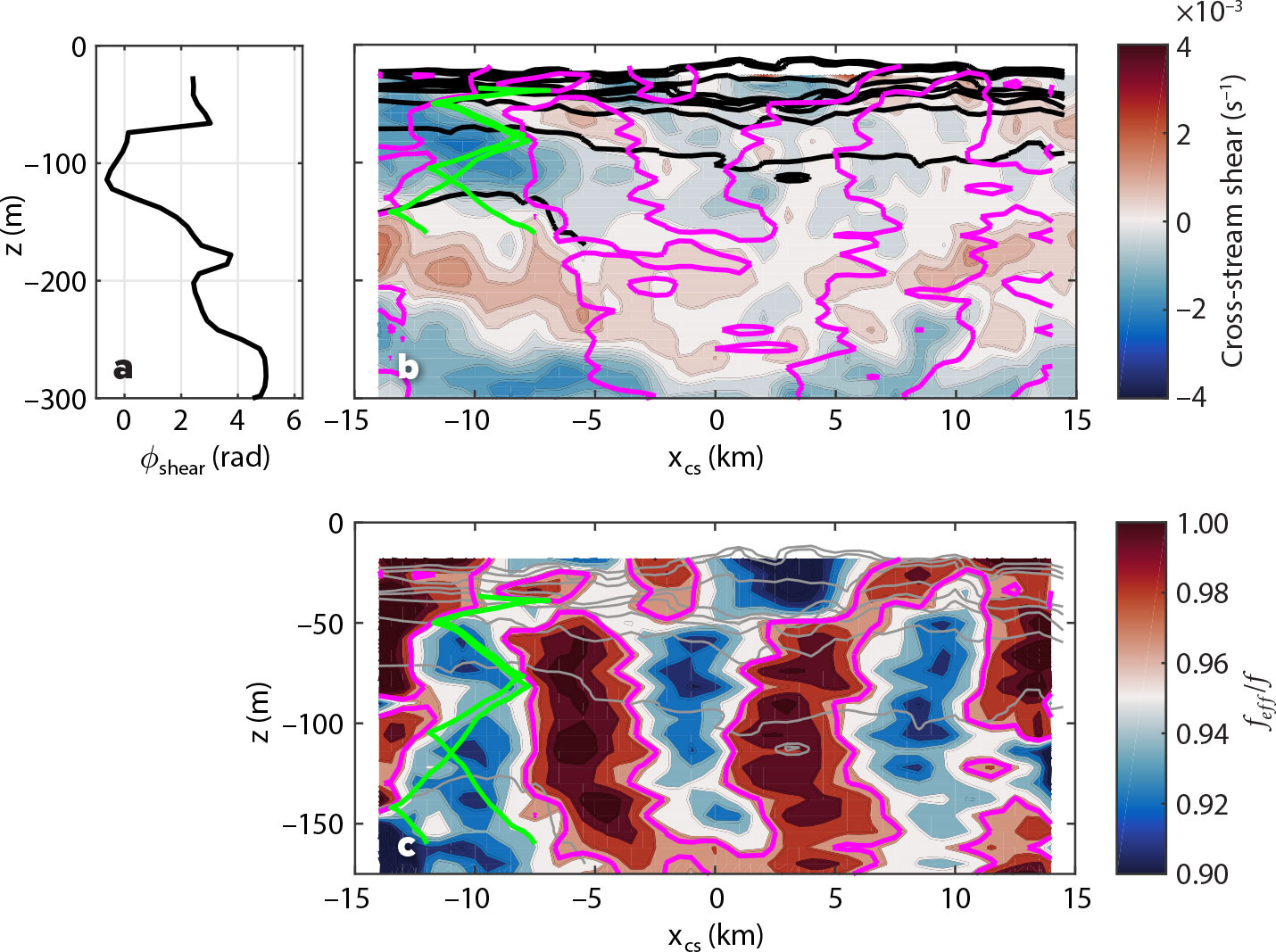
FIGURE 4. Evidence for upward-propagating NIWs from the section indicated by the thick black line in Figure 3a,b, collected between 17:45 and 20:15 June 11, 2019, UTC. (a) Angle that the vertical shear vector makes as a function of depth, ϕshear = tan−1 (vz/uz) evaluated at xcs = –10 km on the section shown in (b). A banded structure is seen in shear near xcs = –10 km (colored in [b]). Beneath 100 m, the shear vector rotates counterclockwise with depth, consistent with upward-propagating NIWs. Two rays (green lines in [b] and [c]) tracing the path of upward-propagating NIWs with a frequency of 0.97f initiated at z = –156 m laterally reflect off locations where the effective inertial frequency is equal to the frequency of the wave, i.e., fe f f = 0.97f (indicated by the magenta contours in [b] and [c]), and converge in the near-surface seasonal pycnocline (isopycnals are contoured in black every 0.05 kg m–3). (c) The effective inertial frequency f + ζ/2 normalized by f (color) and density (contoured at the same interval as in [b]) along the section. > High res figure
|
Ray tracing is a technique used to estimate the path a wave travels in an inhomogeneous medium (Lighthill, 1978). It involves using the dispersion relation for the particular wave of interest to calculate the group velocity and its variations in space. The group velocity can be integrated in time to trace the path of the wave, known as a ray. For NIWs in a background flow, the dispersion relation depends on stratification, the effective inertial frequency, fe f f, and other factors related to the vertical shear of the background flow, which are of secondary importance for this particular anticyclone (Mooers, 1975; Kunze, 1985; Whitt and Thomas, 2013). If the waves have any along-stream propagation, there may be Doppler shifting, which can distort ray paths (Olbers, 1981). To simplify the analysis, we assume that the waves only propagate in the across-stream and vertical directions and neglect Doppler shifting.
On the section of interest described above, there are large variations in stratification and more subtle, although significant, modulations in fe f f that can affect the propagation of NIWs. The effective inertial frequency, like vorticity, covaries with the salinity. In particular, regions where fe f f < f tend to coincide with the saltier filaments (e.g., near xcs –10, 0, 10 km in Figures 3c and 4c). We focus the ray-tracing calculation on the saltier filament centered around xcs = −10 km since this is where the NIW beam is observed. According to the dispersion relation for NIWs, internal waves with a subinertial frequency of 0.97f are permitted in this region where fe f f < 0.97f. The rays of these subinertial waves are trapped in the filament and reflect off their separatrix, i.e., the fe f f = 0.97f surface (Figure 4b,c). This suggests that these saltier filaments with anticyclonic vorticity funneled upgoing NIW energy. In this sense, we might consider these regions to act as inertial chimneys. The rays that propagate upward and outward (i.e., toward decreasing xcs) run nearly parallel to the shear bands, implying that the observed NIWs have an intrinsic frequency close to 0.97 f. These waves would be evanescent in regions where fe f f < 0.97f such as the fresher filament with more positive vorticity near xcs = –5 km. The weakening of the vertical shear there supports this notion (Figures 3c and 4b,c).
Anticyclonic vorticity anomalies in the saltier filaments weaken within the seasonal pycnocline. This vertical vorticity structure has potentially important consequences for the amplitude of upward-propagating, subinertial NIWs. The increase in ζ toward the surface bends the separatrix for these waves into a concave-down shape. This geometry, combined with increasing stratification in the seasonal pycnocline, focuses rays. Such laterally focusing reflections amplify internal waves. In addition, amplification could also arise from a vertical critical layer at the top of the filament if the NIWs cannot escape its confines. Having said this, these interpretations should only be considered suggestive since the assumptions used in the ray-tracing calculation may not hold for this flow (i.e., the lateral wavelengths of the NIWs appear to be larger than the filament widths and Doppler shifting may not be negligible). However, if there is NIW focusing in the filaments, and if the amplification is sufficiently large, it could trigger wave breaking and turbulence. There is evidence for this in the observations.
Enhanced Mixing Atop the Chimney
Microstructure measurements from the GusT probe mounted on Triaxus suggest that the upward-propagating NIWs observed in the section generate turbulence. Sections of potential density (Figure 5b) and squared current shear (Figure 5c) are overlain by colored dots indicating the magnitude of ε along the Triaxus trajectory. These indirect estimates of ε based on fast thermistor measurements cannot be made in the absence of stratification. Hence, mixed-layer values, for example, are flagged so that they are not plotted or included in averages. For reference, the red line in Figure 5e represents an estimate of what we might expect for tendencies of ε in the mixed layer, based on law-of-the-wall scaling using the measured wind-stress to determine the friction velocity u*. The latter is an underestimate near the surface as it does not account for the effects of surface wave breaking and other surface processes and perhaps an overestimate at greater depths where stratification acts to suppress the law of the wall.
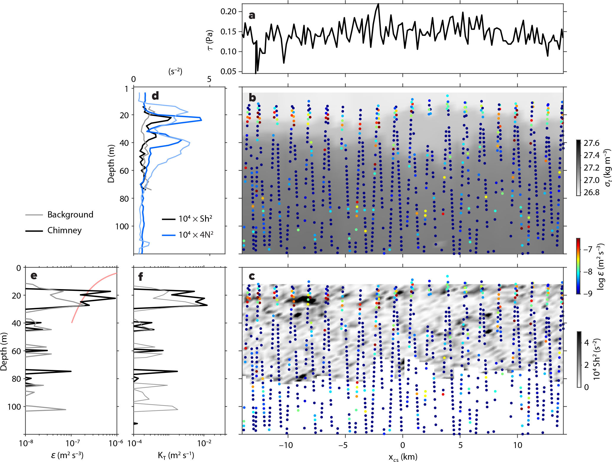
FIGURE 5. Enhanced dissipation and mixing associated with the upward-propagating NIW in Figure 4b. (a) wind-stress, τ, time series. (b) Depth-cross stream section of potential density, σt (gray scale). Colored dots in (b) and (c) represent 5 m depth-averaged estimates of ε from GusT probe on Triaxus. (c) Depth-cross stream section of squared current shear, Sh2 = uz2 + vz2, from 300 kHz ship-mounted ADCP (gray scale). The ADCP is range-limited to 60–80 m in these waters. Colored dots representing ε in (b) are echoed in (c). Vertical profiles of (d) 104 × Sh2 (black), 4N2 (blue), (e) ε, (f) KT. In (d–f), thick lines represent spatial averages over [–15 –5] km representing the region of the inertial chimney (Figure 4); thin lines represent the background average over [–5 15] km. In (e), the red line indicates a law-of-the-wall scaling for ε in the mixed layer where thermistor estimates of ε are not reliable. > High res figure
|
At the base of the mixed layer and above the concave-down separatrix (indicated by the fe f f = 0.97f contour in Figure 4b,c) over xcs = [–15 –5] km (the top of the chimney) lies a region of enhanced ε and Kt relative to background values (Figure 5f). Here, average dissipation rates approach 10–6 m2 s–3, which is nearly 10 times larger than ε averaged across the surrounding waters. Shear and stratification are stronger above the chimney as well. At the mixed-layer base, average N2 is greater by a factor of about 2 while average Sh2 = uz2 + vz2 is greater by more than a factor of 4, bringing the average Richardson number, Ri, nearer to 1/4, or tending reduced shear Sh2 – 4N2 to values > 0, suggesting significant potential for shear instability (Figure 5d). The true vertical resolution of horizontal velocity shear estimated from the 300 kHz ADCP is coarser than its 2 m bins; therefore, Sh2 is likely underestimated so that actual values of Ri may be smaller and reduced shear greater than suggested by Figure 5d.
While small peaks in turbulence have been observed at the bases of ocean mixed layers (Lombardo and Gregg, 1989; Anis and Moum, 1994), observed values of ε approaching 10–6 m2 s–3 and KT > 0.03 m2 s–1 there are greater than previously reported, at least in open ocean conditions away from the equator. We also note that the surface buoyancy flux during this period associated with surface cooling is smaller than the averaged value of ε at the mixed-layer base by a factor of 10. A turbulent diffusivity of 1 × 10⁻² m2 s–1 would mix a layer 10 m thick in 2.5 hours. The fresher waters in the mixed layer observed above the streamer of fresh water in the pycnocline in the high dissipation region (e.g., Figure 3c, xcs < –10 km) could be a consequence of such mixing.
It seems plausible that the enhanced turbulence at the mixed-layer base atop the chimney (Figure 4) derives its energy from the upward propagating NIWs. If so, in a steady state, dissipation would be balanced by convergence of the wave energy flux, Fe (similar to what Kunze et al., 1995, found for downward-propagating NIWs approaching a critical layer at the base of a Gulf Stream warm-core ring). With this balance in mind, integrating the dissipation profile in the vertical can yield an upper bound on the wave energy flux needed to sustain the dissipation (i.e., Fe = ∫z0ρ0εdz). Estimates of ε in the mixed layer are set to zero in this integral, because ε is not well constrained in the mixed layer and the objective of this calculation is to quantify the jump in wave energy flux in the seasonal pycnocline that would drive the inferred enhanced dissipation there. The integration implies that an upward wave energy flux of order 10 mW m–2 would have to be absorbed in the seasonal pycnocline to support the observed dissipation if no other sources of energy were available for the turbulence. The plausibility of an NIW energy flux of this magnitude, given the properties of the NIW field in the Iceland Basin, is discussed in the last section of this article.
Possible Sources of the Upward-Propagating NIWs
We now attempt to constrain the origin of the upward-propagating NIWs observed on the section. Three hypotheses are explored: (1) upward radiation of semi-diurnal internal tides (which are near-inertial at these latitudes), (2) reflection of wind-driven NIWs off the bottom, and (3) reflection of wind-driven NIWs off jumps in stratification.
Semi-Diurnal Internal Tides
Semi-diurnal internal tides have been observed to emanate from the nearby Reykjanes Ridge (Vic et al., 2021). At the latitude of the survey, semi-diurnal tides have a frequency of 1.13f which, although close to f, would generate NIWs with shear bands of slope  roughly twice as large as the observed slope for an intrinsic frequency ωi = 1.13f. However, it is possible that the intrinsic frequency of the semi-diurnal tides could be modified by the mean current of the anticyclone through a Doppler shift. In particular, if ωi were shifted below f, then the shear bands could be attributed to semi-diurnal tides. For this to happen, the internal tide would need to propagate with the mean current and have a wavelength of a few hundred kilometers in the along-stream direction. It is possible that these conditions were met in the anticyclone. For example, if the semi-diurnal tides were radiated directly from the Reykjanes Ridge, they would most likely propagate with the eastward mean current on the northern edge of the anticyclone because the ridge is to the west of the eddy. Thus, we cannot rule out the semi-diurnal internal tides as a source of energy for the observed upward-propagating NIWs.
Reflected Wind-Driven Near-Inertial Waves
Alternatively, if the NIWs were driven by winds at the surface, the upward-propagating waves that we observed must have reflected off either an interior fluid boundary or the seafloor. We use wave travel time to determine which scenario is more plausible under the assumption that the NIWs on the section were generated by the strong wind event on May 30, 2019, when a large amount of near-inertial energy was injected into the ocean (Figure 2c) followed by downward-radiating NIWs (Thomas et al., 2020, 2023), and not an earlier storm. This wind-event occurred ~12 days prior to the measurements of the upward-propagating NIWs. Therefore, reflection scenarios with wave travel times that significantly exceed 12 days are ruled out.
Travel times were estimated using ray tracing. For this calculation, hydrography from the deep CTD cast closest to the center of the anticyclone was used for the stratification (Figure 6c). A downgoing ray was initiated at a depth of 150 m with a vertical wavelength of 400 m and subinertial frequency 0.97f. We assume that vorticity of the background flow is uniform with a value of –0.1f and the stratification is laterally homogeneous. With these wave parameters and background flow, ray tracing predicts that in 12 days an NIW packet only reaches a depth of 700 m, which is well short of the bottom at ~3,000 m (Figure 6a). A wave with vertical wavelength shorter than 400 m, more similar to what was observed by Thomas et al. (2020) shortly after the May 30 wind event, would travel even more slowly. Thus, we can eliminate bottom reflection as the source of the observed upward-propagating NIWs, if the waves were forced by the May 30 wind event. If the waves were forced by an earlier storm, however, bottom reflection of NIWs cannot be discounted.
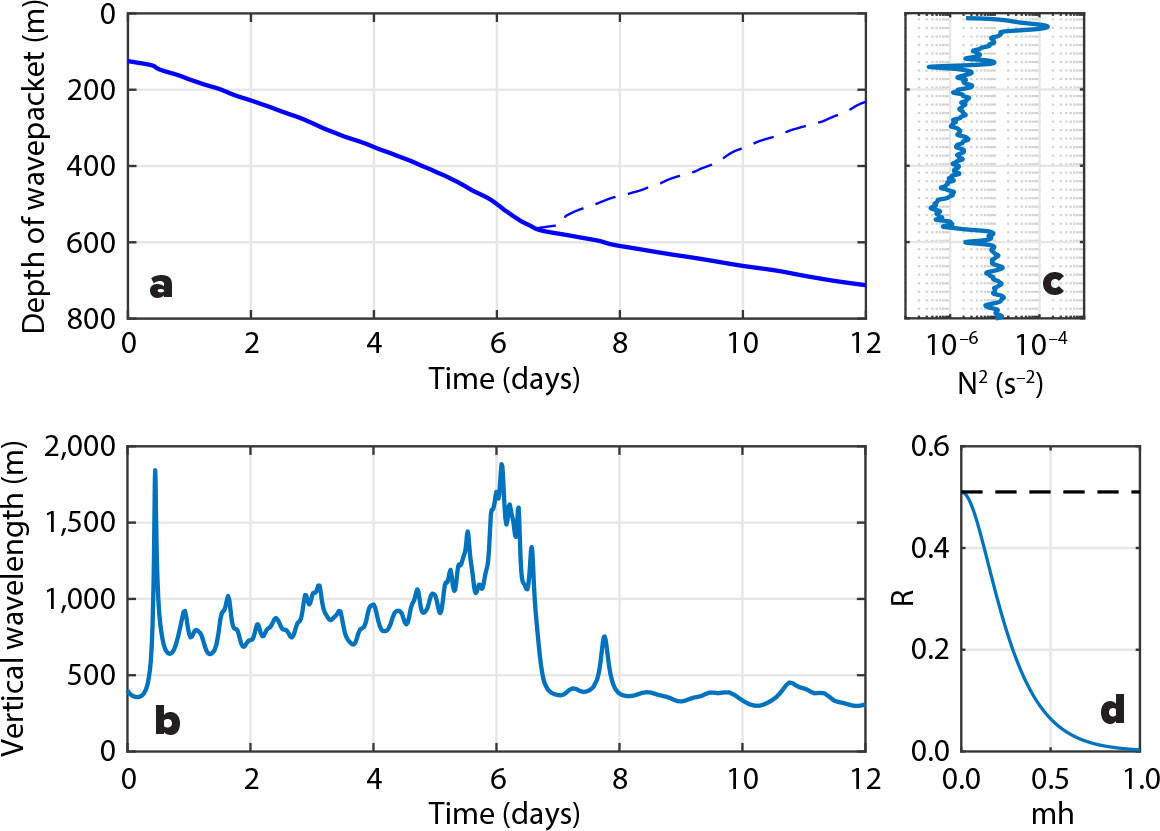
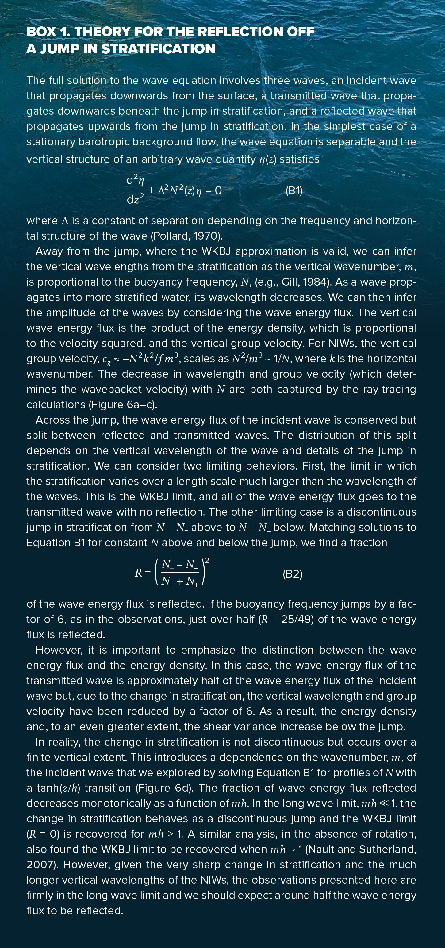
FIGURE 6. Ray-tracing estimates of travel time and vertical wavelength of an NIW with frequency 0.97f propagating in an anticyclone with vorticity −0.1f and stratification representative of the observations. Depth (a) and vertical wavelength (b) of an incident and transmitted (solid blue) and reflected (dashed blue) NIW wavepacket as a function of travel time. (c) Stratification profile within the anticyclone at 58°5’N, 22°10’W that was used in the ray-tracing calculation, with an abrupt jump at a depth near 600 m affecting wave properties. (d) Fraction of the wave energy flux reflected by a smooth sixfold increase in buoyancy frequency as a function of mh where m is the incident wavenumber and the buoyancy frequency increases with a tanh(z/h) transition region. The gray dashed line indicates the fraction reflected by a discontinuous sixfold jump (Equation B2). > High res figure
|
Ray tracing also predicts that the vertical wavelength of the NIW increases from its initial value of 400 m as the NIW transits the weakly-stratified core water, then sharply decreases from ~1,500 m to less than 500 m when the wave crosses the jump in stratification near 600 m (Figure 6b). This change in wavelength occurs over a distance much smaller than the wavelength itself, which is in clear violation of the WKBJ approximation that forms the basis of ray tracing. Therefore, in the proximity of jumps in stratification of this magnitude, ray tracing should not be used to infer properties of the wave field, but instead full solutions to the wave equation should be sought. Such solutions have been calculated for similar stratification profiles and predict that a fraction of the downward-propagating wave energy is reflected off jumps in stratification (see Box 1).
Reflection off Stratification Jump: Idealized Simulations
To further illustrate the plausibility of reflection of wind-driven NIWs off the stratification jump at the top of the permanent pycnocline at 600 m as the source of the upward-propagating NIWs, we ran idealized simulations to illustrate the mechanism using the Regional Ocean Modeling System (ROMS; Shchepetkin and McWilliams, 2005). The model domain is 240 km × 9 km with a uniform depth of 2,400 m. Horizontal resolution is 500 m × 500 m, and there are 256 depth layers. The depth grid is surface refined so that the spin-up of near-inertial motions near the surface can be captured. The Coriolis frequency is constant and set to f at 58°N. The background velocity is a double jet mimicking the azimuthal flow of the observed anticyclonic eddy (see Figure 7a). The domain is set to be extremely narrow in the along-jet direction with few grid points, under the assumption that variation in the along-jet direction is small. The vertical vorticity in this two-dimensional “anticyclone” is –0.05 f. The observed wind-stress from May 29 to June 1 (e.g., Figure 2b) is used to force the model for the first four days, and then wind forcing is set to zero for the remaining six days of the simulation. The background density has two different configurations for comparison. One uses the observed stratification from the deep CTD cast (Figure 6c), and the other uses a modified stratification profile without the stratification jump at 600 m (see Figure 7b).
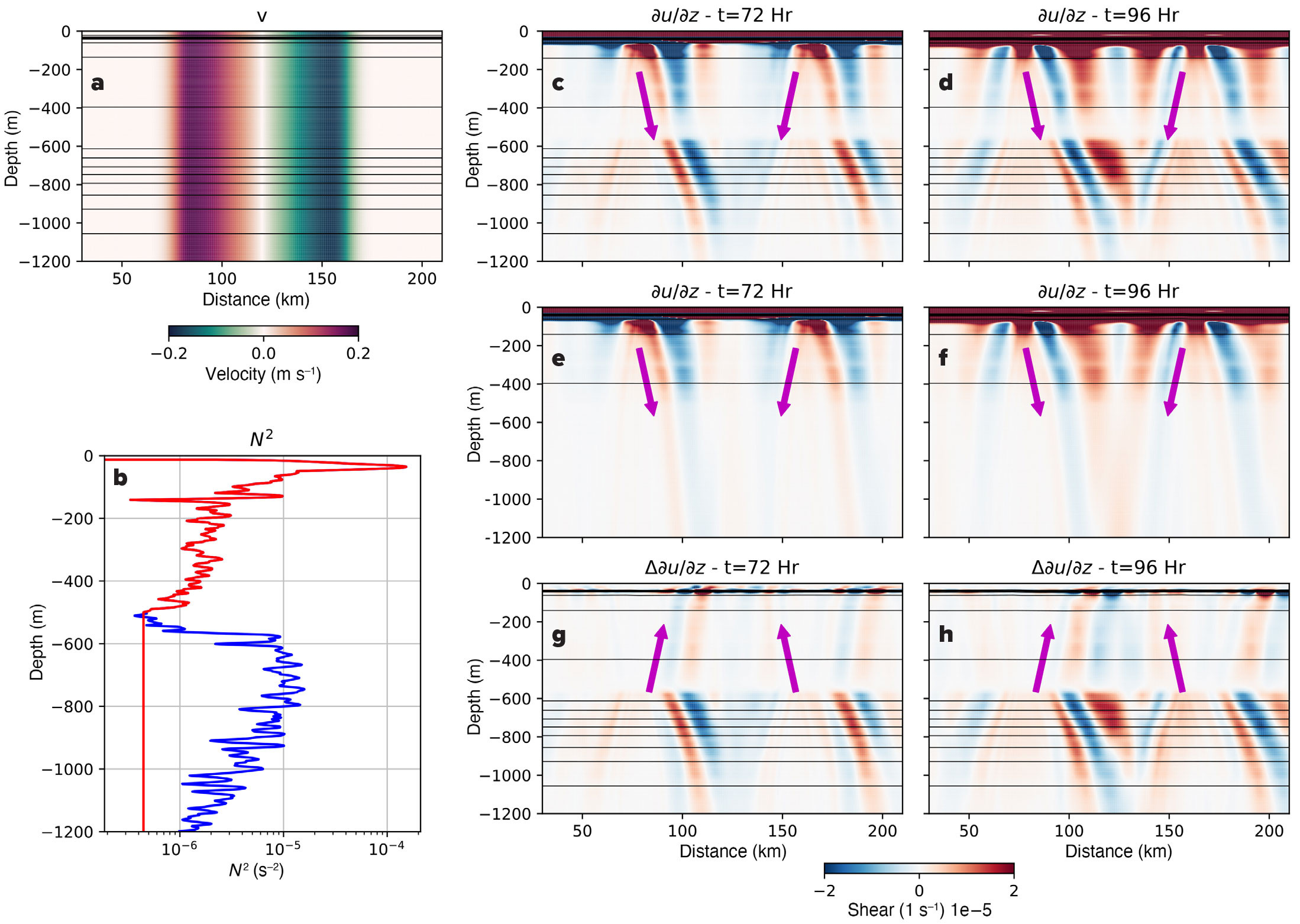
FIGURE 7. Simulations illustrating how NIW generated by winds trapped in an anticyclone can reflect off a jump in stratification. (a) Structure of the velocity of the anticyclone used in the simulations (cross-section velocity, v, is in color). (b) Vertical structure of the square of the buoyancy frequency, N2, for the simulation with (blue) and without (red) a jump in stratification. Snapshots of the vertical shear at 72 and 96 hours into the simulation for the runs with a jump in stratification (c) and (d), without a jump in stratification (e) and (f), and the difference between the two runs (g) and (h). Magenta arrows indicate the direction of energy propagation of NIW beams in shear and shear difference. A supplementary animation of panels (c) to (h) can be found at https://youtube.com/shorts/sJd8eDpMXL8. > High res figure
|
Within the anticyclone (i.e., between 90 and 160 km), vertical shear takes a banded structure, with the shear bands tilting down and toward the center of the anticyclone, a feature characteristic of NIWs trapped in an inertial drainpipe (Figure 7c–f). There are also downgoing NIWs outside of the anticyclone. These are associated with NIWs that radiate away from the regions of cyclonic vorticity on the outer edges of the jet. The difference in shear between the simulation with and without the stratification jump quantifies adjustments to the NIW field due to the abrupt change in N2. Above the permanent pycnocline (z > –600 m), a pattern consistent with upward-propagating NIWs is visible, with shear bands that tilt up and toward the center of the anticyclone (e.g., Figure 7g,h).1 Three days into the simulation (corresponding to two days after the wind event on May 30), a NIW that had reflected off the stratification jump has returned to the surface (e.g., Figure 7g). This NIW has a long vertical wavelength (~1,200 m) and propagates rapidly. An NIW with a 200 m vertical wavelength similar to the observations (e.g., Figure 4b) would propagate at one sixth the speed of this NIW (if the frequencies of the waves were the same), implying that a NIW with a 200 m vertical wavelength would reach the surface ~12 days from the wind event after reflecting off the jump in stratification, a time scale consistent with the observations.
The locations where the upgoing NIWs in the anticyclone reach the surface (~120 km and ~140 km) are toward the center of the eddy, unlike the observed upgoing NIWs that were found near the edge of the eddy. These locations are set by the particular paths along which NIWs propagate. These ray paths are sensitive to many factors, such as the detailed spatial structure of vorticity and stratification in the eddy and its filaments and the horizontal direction waves propagate (which might not be perfectly radial), factors that are not expected to be captured in these idealized simulations. The objective of these simulations is not to determine the locations where the upgoing NIWs reach the surface, but to demonstrate how NIWs can reflect from a jump in stratification representative of the observations.
1 To better visualize the propagation of the NIWs in the simulations, see the supplementary animation of Figure 7 panels c–h at https://youtube.com/shorts/sJd8eDpMXL8.
Discussion
Assuming that the observed upward-propagating NIWs are wind-driven NIWs reflecting off the seasonal pycnocline, the question still remains of whether such waves are sufficiently energetic to explain the high dissipation rates at the base of the mixed layer observed within the NIW beam. If balanced by an influx of wave energy into the seasonal pycnocline, it was shown above that the inferred dissipation would require a wave energy flux of order 10 mW m–2. Downward NIW energy fluxes shortly after the wind event on May 30, 2019, are an order of magnitude weaker than this (Thomas et al., 2023). In addition, NIWs are only partially reflected off a stratification jump of the strength seen at 600 m. As discussed above, the upward energy flux of the reflected waves should be around half the energy flux of the downgoing NIW and would correspond to a fraction of a mW m–2. However, these waves could still power the observed dissipation if wave focusing in filaments locally intensifies the NIWs to a sufficient degree. For this to happen, the cross-sectional area of beams of upward-propagating NIWs would have to shrink by more than a factor of ten as they transit from the permanent pycnocline to the top of the ~5 km wide vorticity filaments. The two-dimensional, idealized simulations suggest that beams of upward-propagating NIWs span ~50 km near 600 m (Figure 7h), approaching the tenfold larger widths needed to support the requisite intensification in energy flux near the surface.
The observations, theory, and simulations described here paint a different picture of NIW behavior in anticyclones than the conceptual models of inertial drainpipes and critical layers at the bases of anticyclones. Namely, the energy sink for NIWs in anticyclones can shift to the upper ocean when downward-propagating NIWs reflect off the permanent pycnocline and are focused, amplified, and dissipated in filaments of anticyclonic vorticity. The reflection partially blocks an inertial drainpipe, and the submesoscale, anticyclonic filaments that focus the upward-propagating NIWs act like a surface-layer waveguide that could be described as an inertial chimney.
Clearly, this NIW behavior is shaped by the particular characteristics of the anticyclone we observed, specifically, an abrupt transition in stratification between a well-mixed remnant winter water layer and the permanent pycnocline that is located higher in the water column than the critical layer, and submesoscale filaments of vorticity that weaken in magnitude towards the surface. Having said this, anticyclones are often characterized by core waters with anomalously weak stratification bounded below by a stratified layer (e.g., Gulf Stream warm-core rings and mode-water eddies), and filamentation of vorticity on the edge of eddies is common. Thus, the confluence of conditions that we observed may not be too unusual. In the Japan/East Sea for example, there have been observations of upward-propagating NIWs in anticyclones with a similar stratification profile to that described here (Byun et al., 2010).
In the Iceland and Irminger Basins, two consecutive years of velocity profiles made with floats spread throughout the region show a widespread dominance of upgoing NIWs in June through August (Kunze et al., 2023). These floats sampled many different mesoscale environments, not just anticyclones, so the NIWs observed by the floats likely took a variety of propagation pathways different from the ones discussed in this article. The near-inertial signals measured by the floats could have been associated with semi-diurnal internal tides radiated from topographic ridges, a scenario that might also explain the upward-propagating NIWs that we observed (if they were Doppler shifted). It should be noted that the analyses of Kunze et al. (2023) were primarily focused on depths within the permanent pycnocline where reflections of downward-propagating NIWs off the top of the pycnocline are not obviously relevant. Nevertheless, the observations from the floats highlight how the combination of a weakly stratified winter water layer and a concomitant jump in stratification in the permanent pycnocline is a ubiquitous feature of the hydrography in the Iceland and Irminger Basins, and so may lead to reflections of downgoing NIWs across the basin.
Globally, it is estimated that the shear variance in downgoing internal waves exceeds the shear variance in upgoing waves by 30% in the upper 600 m of the ocean (Waterhouse et al., 2022). This implies that there is considerable energy in upward-propagating internal waves in the upper ocean. The source, fate, and regional variations of such waves is not well understood. The mechanisms that we have described here involving mesoscale eddies, internal reflections off jumps in stratification, and wave focusing in filaments of vorticity could contribute to shaping the submesoscale structure of the upgoing NIW and turbulence fields in the ocean. Quantifying their regional and global impacts would be of interest.
Acknowledgments
We are grateful to the captain and crew of R/V Neil Armstrong who made the collection of these observations possible. This work was supported by ONR Grants N00014-18-1-2798 (L.N.T.), N00014-18-1-2780 (L.R. and C.M.L.), N00014-18-1-2788 (J.N.M.), and N00014-18-1-2398 and N00014-18-1-2801 (E.K.) under the NISKINe Directed Research Initiative. Comments from Amanda Vanegas Ledesma helped to improve the article.