Introduction and Setting
In 1990, the German oceanographer Detlef Quadfasel went as tourist on a cruise on the Soviet icebreaker Rossiya to the North Pole, taking with him expendable temperature probes. He discovered that the temperature of the mid-depth Atlantic layer was more than one degree above that reported from previous measurements (Quadfasel et al., 1991). This observation drastically changed the focus from determining the mean circulation and water mass structure to detecting and documenting change. Subsequent expeditions in the following decade revealed changes also in water mass structure (Steele and Boyd, 1998; Morison et al., 1998), frontal zone locations (Carmack et al., 1995), currents, and response to atmospheric forcing (Maslowski et al., 2000). A comparison of submarine upward-looking sonar tracks of the ice cover 30 years apart showed that the ice cover thickness had been reduced by almost half (Rothrock et al., 1999). Gone was the concept of a steady state ocean, and to detect, study, and understand change became a major goal of Arctic research.
Many of the observed changes were advective, related to the inflow of Atlantic and Pacific waters as well as to the warming climate. The northward advection of warmer air, containing more clouds and water vapor, increases the downward longwave radiation that causes higher surface temperatures (Mortin et al., 2018), and the inflow of warmer Atlantic water provides more heat to the upper layer beneath the ice (Polyakov et al., 2012a). Rivers flowing north from the massive, surrounding continental drainage basins add a third advective component. All these transports affect the ice cover, causing melting or inhibiting freezing.
The Arctic Ocean’s polar-centric location means that it is affected seasonally by the most variable radiative forcing of all oceans: during the polar night, the air temperature may sink below –40°C, and the continuous daylight at summer solstice provides more shortwave radiation at the top of the atmosphere than that received at the equator. It is mostly a β ocean, that is, strongly stratified in salinity but not always in temperature. Winter cooling is thus confined to a strongly stratified and relatively shallow surface layer, allowing the surface to reach freezing temperature and form sea ice. The local, oceanic heat given up to the atmosphere and to space is then latent heat of freezing, not sensible heat stored in the water column, and the overlying atmosphere becomes colder than it otherwise would be. In summer, the ice cover reflects a substantial fraction of the incoming shortwave solar radiation, and the melting ice keeps the surface temperature close to freezing, thus making the summer cooler than expected, considering the many hours of sunlight the Arctic Ocean receives during this season.
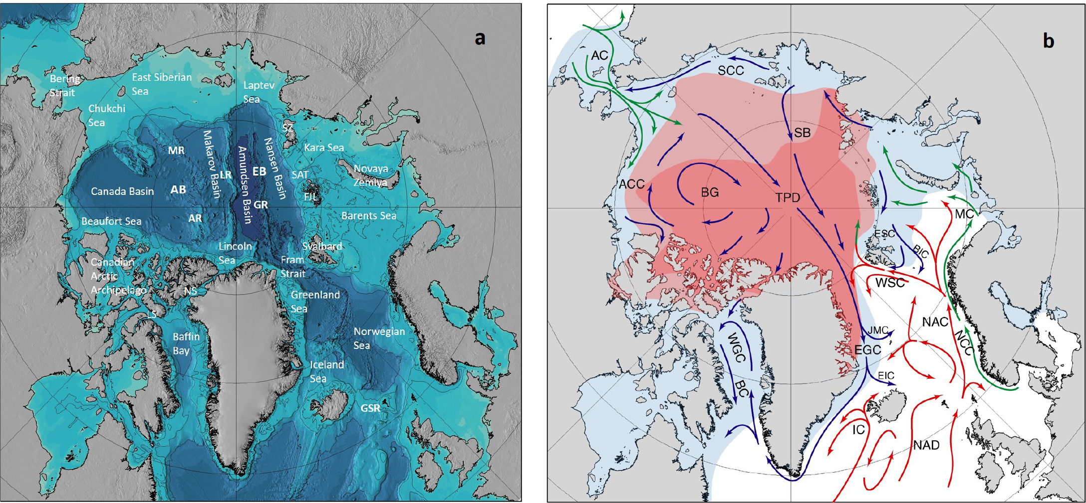
The Arctic Ocean is also unique among global oceans in that its shelves comprise approximately 50% of its area, so seasonal modifications of water masses are amplified. With mean depths ranging from 200 m to less than 50 m, the shelves are geographically separated into the Barents, Kara, Laptev, East Siberian, and Chukchi Seas north of the Eurasian continent, and the Beaufort Sea, Lincoln Sea, and Canadian Arctic Archipelago north of North America. The deep part of the Arctic Ocean consists of two major basins, the Eurasian and Amerasian Basins, which are physically separated by the Lomonosov Ridge with a mean depth of 1,600 m and a sill depth of 1,870 m. The Eurasian Basin is further divided by the Gakkel Ridge into the 4,500 m deep (the average depth of the abyssal plain) Amundsen Basin and the 4,000 m deep Nansen Basin, and the Mendeleev Ridge and the Alpha Ridge system separate the Amerasian Basin into the smaller 4,000 m deep Makarov Basin and the larger 3,800 m deep Canada Basin (Figure 1a).
|
Circulation and Stratification: From the Bottom Up
The advective flows into the Arctic Ocean have long been recognized. In the mid-nineteenth century, the possibility that these warm inflows could influence the ice cover and create open water in the interior of the Arctic Ocean was seriously discussed (Petermann, 1865; Bent, 1872). Fridtjof Nansen’s drift with Fram demonstrated that this was not the case, but instead a warm layer with temperatures above 0°C was present between 150 m and 600 m depth, showing that warm Atlantic water does enter the Arctic Ocean; however, it is separated from the sea surface by a low salinity upper layer that prevents its heat from reaching the ice (Nansen, 1902).
This strong, permanent stability is created by the global-scale atmospheric transfer of water vapor from lower to higher latitudes, and in the Arctic Ocean the local net precipitation is augmented by its large continental catchment areas, which deliver over 10% of the global river runoff. The Arctic Ocean becomes a β (salt-stratified) ocean (Carmack, 2007), and the resulting stability isolates the underlying water column from surface forcing so that it is dominated by advection. Exchanges between the upper and the deep ocean are only possible via the shallow shelves and the upper slope, or by inputs from adjacent seas.
That sea ice formation on the shelves could be important for the ventilation of the deeper layers of the Arctic Ocean was first argued by Nansen, ironically based on erroneous salinity determinations from the Fram expedition, which showed that the salinity of the deep waters was higher than that of Atlantic water. He suggested that freezing and brine rejection on the shelves could explain these high salinities. However, Nansen later suggested, based on Amundsen’s Gjøa observations in 1901, a role for the deep open ocean convection occurring in the Greenland Sea, and he eventually accepted the possibility that the deep and bottom water in the Arctic Ocean originated in the Greenland Sea (Nansen, 1906, 1915).
This description of the deep circulation in the Arctic Ocean and the Nordic Seas, elaborated with more observations by Wüst (1941), was accepted for more than 50 years. When Worthington (1953) found that the temperatures below 1,300 m were lower in the eastern (Eurasian) half than in the western (Amerasian) half of the Arctic Ocean, he concluded that a submarine ridge must divide the Arctic Ocean in two basins, preventing the coldest, densest water from the Greenland Sea from reaching the western Arctic Ocean. This ridge, the Lomonosov Ridge, had, unknown to Worthington, been detected by Soviet scientists in 1948. It was not until Aagaard (1980) pointed out that the Amerasian Basin deep water was not only warmer but also more saline than the Eurasian Basin deep water that Nansen’s shelf source suggestion was considered anew (Aagaard et al., 1981, 1985; Rudels, 1986). It is now accepted that the deep circulation in the Arctic Ocean and in the Nordic Seas forms a tightly linked system, with the Arctic Ocean shelves providing the warm/saline and the Nordic Seas the colder/fresher end members.
The deep and bottom water masses in the Arctic Ocean’s four deep basins each have their own distinct characteristics. The coldest bottom water occurs in the deepest basin, the Amundsen, with a potential temperature of –0.94°C and salinity around 34.943. The bottom water in the shallower Nansen Basin is slightly warmer but less saline, while the bottom water in the Canada basin is clearly warmer, –0.551°C, and more saline, 34.958. The vertical structures of the deep waters in these three basins are similar. Temperature decreases and salinity increases down to about 1,000 m from the bottom, where the temperature starts to increase with depth, creating a deep temperature minimum. The temperature and salinity increase until a thick homogeneous bottom layer, capped by a thermohaline step structure, is reached; these layers are 1,000 m thick in the Canada Basin and about 600 m in the Amundsen Basin and 500 m in the Nansen Basin (Figure 2).
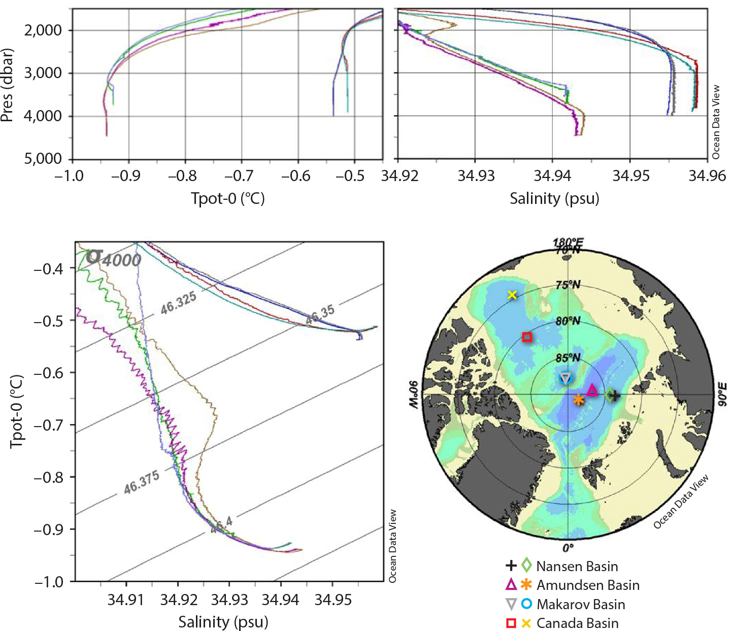
FIGURE 2. Deep and bottom water characteristics from the Nansen, Amundsen, Makarov, and Canada Basins. Green = Nansen Basin (diamond on map). Purple = Amundsen Basin (triangle). Gold = Makarov Basin (asterisk). Red = Canada Basin (square). Green = Canada Basin (x). Note the absence of a deep temperature minimum in the Makarov Basin and that the temperature minimum in the Canada Basin could be caused by an inflow at sill depth from the Makarov Basin. The deep (2,000 m) salinity maximum in the Amundsen Basin is likely caused by Makarov Basin deep water crossing the Lomonosov Ridge. The temperature minima in the Nansen and Amundsen Basins have no obvious advective sources but could be caused by intermittent inflow of colder water via the St. Anna Trough or by varying characteristics of the Fram Strait inflow branch. From Rudels (2012). > High res figure
|
The temperature and salinity increase toward the bottom can be explained by shelf/slope convection. The inflow through Fram Strait comprises warm, saline Atlantic water and less saline and colder intermediate and deep water, and the slope convection entrains Atlantic water and becomes warmer. If it is saline enough, it sinks into and increases the temperature and salinity of the advected intermediate water below (Quadfasel et al., 1988).
The deep temperature minimum in the Canada Basin is likely due to spreading of colder water from the Makarov Basin across the Mendeleev Ridge (see profiles in Figure 2). The minima in the Amundsen and Nansen Basins are located deeper than the sill in Fram Strait, have no obvious advective sources, and are more difficult to explain. The temperature of the sinking plumes, once they have passed the Atlantic water, cannot be increased by entrainment, except intermittently, if the salinity and temperature of the inflow change with time. However, the thick, homogeneous bottom layers suggest that geothermal heating could lead to temperature increases, convection, and homogenization of the bottom water (Timmermans et al., 2003; Björk and Winsor, 2006). Observations of the bottom layer in the Canada Basin during the first decade of the twenty-first century indicate that the bottom temperature has increased, supporting the idea of geothermal heating (Carmack et al., 2012).
The structure in the deep Makarov Basin is different. No deep temperature minimum is present, and the salinity reaches its maximum value 1,000 m above the bottom and then remains constant with depth, while the temperature continues to decrease until it forms a 700 m thick bottom layer (Profiles in Figure 2). Jones et al. (1995) suggested that the absence of a temperature minimum was due to spillover of colder intermediate depth water from the Amundsen Basin across the sill in the central Lomonosov Ridge. This water would, due to the thermobaric effect (see later section on Internal Mixing Processes), sink to the bottom and cool the deep water in the Makarov Basin. Later observations (Björk et al., 2007), however, did not confirm such overflow. If it is the cause of the temperature structure in the deep Makarov Basin, the overflow must be intermittent (Rudels, 2012).
Connections with the World Ocean
The largest exchanges between the Arctic Ocean and the rest of the world ocean occur in the North Atlantic. There, warm Atlantic water crosses the Greenland-Scotland Ridge and enters the Nordic Seas (the Greenland, Iceland, and Norwegian Seas), which form a large anteroom for the two Atlantic entrances to the Arctic Ocean, the shallow (200 m) Barents Sea and the deep (2,600 m) Fram Strait. The Atlantic water flows north in the Norwegian Atlantic Current, where strong heat loss to the atmosphere leads to cooling and densification of the entering water. The current splits north of Norway, and a substantial fraction enters the Barents Sea, which makes the southern part of the Barents Sea ice-free throughout the year. The remainder of the Norwegian Atlantic Current continues as the West Spitsbergen Current to Fram Strait, where about half enters the Arctic Ocean and forms a boundary current that follows the Eurasian continental slope eastward. The rest recirculates in the strait and joins the southward-flowing East Greenland Current (Rudels, 1987; Figure 1b).
The Fram Strait inflow branch encounters and melts sea ice north of Svalbard, and its upper part is transformed into a less saline surface layer. The underlying warm “Atlantic” core becomes isolated, and its transfer of heat to the atmosphere is reduced. Rudels et al. (2004) assumed that the upper layer is created by sea ice melting and wind mixing and that the heat loss of the Atlantic water is distributed between the atmosphere and sea ice in such a way that the amount of sea ice melting is a minimum. This is actually the distribution requiring the least energy input from the wind to turbulent mixing (Rudels, 2016). The Barents Sea branch, by contrast, does not meet sea ice until it reaches the northeast corner of the Barents Sea, where it continues into the Kara Sea between Franz Josef Land and Novaya Zemlya. The temperature of the Atlantic water in the Barents Sea is then lower than that of the Fram Strait branch, which leads to a smaller fraction of the heat loss going to ice melting, and the salinity decrease in the created upper layer is less than in the corresponding layer north of Svalbard (Rudels et al., 2004).
The Arctic Ocean is not a closed bay. Rather, it has a narrow (80 km) and shallow (50 m) backdoor, Bering Strait, to the opposite part of the world ocean, the North Pacific. The North Atlantic is weakly stratified in temperature (α ocean) and well ventilated, while the North Pacific is strongly stratified in salinity (β ocean) and poorly ventilated below its seasonal pycnocline. Its upper layer is less saline, partly due to transfer of water vapor from the Atlantic across the Isthmus of Panama (Weyl, 1968). This leads to higher sea level in the North Pacific compared to the North Atlantic, forcing a northward barotropic flow of low salinity water through Bering Strait into the Arctic Ocean (Stigebrandt, 1984). After transiting the Chukchi Sea, the flow interleaves around 75 m depth in summer and about 150 m in winter between the low salinity surface layer and the Atlantic waters below, augmenting the already strong upper layer stability.
Beyond the Nansen Basin, the upper layers in the deep ocean basins are dominated by freshwater input, either from rivers or from the Bering Strait inflow. Only in the Nansen Basin do direct interactions between sea ice and warm entering water create a less saline upper layer that leads to higher density and weaker stability there than elsewhere in the Arctic Ocean.
The entering waters become transformed within the Arctic Ocean and eventually leave to the North Atlantic either through the shallow straits and channels in the Canadian Arctic Archipelago, mainly through Lancaster Sound and Nares Strait, or through Fram Strait in the East Greenland Current. Most of the waters derived from the Pacific inflow pass through the Archipelago, while the East Greenland Current comprises waters drawn from the entire water column, low salinity upper waters that intermittently include Pacific water, cooled Arctic Atlantic water, and intermediate and deep waters from the different basins. These waters become modified and augmented by mixing with the Atlantic water recirculating in Fram Strait and with the water masses in the central Greenland and Iceland Seas before they cross the Greenland-Scotland Ridge, either as low salinity polar water in the East Greenland Current or as dense overflows passing through Denmark Strait or the Faroe Bank Channel into the deep North Atlantic.
Circulation in the Arctic Ocean: Wind Forcing
The Upper Layers
The circulation in the Arctic Ocean is forced mechanically by the wind and by density changes caused by cooling and heating, by freezing and melting, and by freshwater input. The wind-driven Ekman transport dominates in the surface layer. Sea ice and the uppermost layer are mainly driven directly by the wind, but also by the dynamical topography created by the spatially varying Ekman transports. The large-scale wind field over the Arctic Ocean forces a clockwise circulation in the Amerasian Basin, centered at the Beaufort Sea, and a counterclockwise circulation over the western Siberian shelf and the Nansen Basin along the tracks of the low-pressure systems arriving from the North Atlantic. At the boundary between the two wind systems, the counter-rotating winds drive the TransPolar Drift, carrying sea ice and low salinity water from both the eastern Siberian shelves and the Beaufort Gyre toward Fram Strait. As the TransPolar Drift approaches the strait, it splits, with some water returning to the Beaufort Gyre and the rest continuing through Fram Strait. During the transit across the Arctic Ocean, waters are exchanged between the two wind-driven circulation systems (Figure 1b).
The variability of the overall atmospheric circulation is often described by the Arctic Oscillation (AO) index (Thompson and Wallace, 1998). It is a measure of the strength of the Polar Vortex, and an AO+ indicates a strong, tight vortex and an anticlockwise driving of the upper layer and a reduced Beaufort Gyre. By contrast, in the AO– situation, the clockwise circulation is strong and the Beaufort Gyre expands, keeping most of the Pacific inflow in the Amerasian Basin (Steele et al., 2004). In the AO+ situation, the weakened Beaufort Gyre allows the anticlockwise circulation in the Eurasian Basin to extend farther east, and some of the Pacific inflow is carried directly into the Eurasian Basin to exit through Fram Strait (Steele et al., 2004). At the same time, deeper lying waters from the Eurasian Basin shelves are forced across the Lomonosov Ridge to eventually enter the Beaufort Gyre (Morison et al., 2012).
The Barotropic Wind-Driven Circulation
Below the low salinity upper layer, the stratification is weak, and the water columns appear to follow the depth contours. In both the Arctic Ocean and the Nordic Seas, the bathymetry forms closed f/H contours, where f is the Coriolis parameter and H the ocean depth. This allows geostrophic barotropic flows to circulate around the basins along the f/H contours (Nøst and Isachsen, 2003). The vorticity added by the large-scale wind field is transferred to the deeper part of the water column, where it is dissipated by frictional bottom torque. The wind fields over the Nordic Seas and over the Eurasian Basin are anticlockwise, and to remove the injected vorticity, the circulation must be anticlockwise, with the shallow water to the right, looking in the direction of the flow. This is the situation in most parts of the Arctic Mediterranean (“Mediterranean” because it is mostly enclosed by land), but in the Canada Basin, the clockwise wind field could induce a clockwise circulation with the shallow water to the left, which occasionally has been reported (Newton and Coachman, 1974; Karcher et al., 2007).
In a theoretical and laboratory study of a two-basin system, Nøst et al. (2008) found that an anticlockwise wind field in one basin, for example, in the Nordic Seas, would generate an anticlockwise flow along the f/H contours in both basins, while clockwise driving could maintain a clockwise flow in the directly driven basin but a clockwise flow extending to the non-forced basin would eventually go unstable. This implies that the deep barotropic circulation in the Arctic Ocean could be forced to follow the f/H contours around the Nordic Sea and the Arctic Ocean by an anticlockwise wind field acting only over the Nordic Sea, dissipating the added vorticity by bottom friction. This circulation model, however, does not consider the strong thermohaline forcing and the transformations of the waters that take place along their pathways in the Arctic Ocean.
Circulation in the Arctic Ocean: Thermohaline Forcing
The Arctic Ocean is a global-scale double estuary (Carmack and Wassmann, 2006) in that the density of the entering Atlantic water both increases and decreases, creating return flows in the upper layers as well as in the deep, as shown schematically in Figure 3. In the Norwegian Sea and in the southern Barents Sea the Atlantic water is cooled and its salinity decreases slightly due to net precipitation. It is still at the surface, but its density has increased sufficiently for it to enter the deep overturning loop. However, when the Atlantic water eventually encounters sea ice in the Arctic Ocean north and east of Fram Strait, it loses heat both to the atmosphere and to sea ice melting. The meltwater added to the upper part of the Atlantic water lowers its density more than it is raised by the simultaneous cooling, and some Atlantic water is shifted into the upper, estuarine loop. For the Fram Strait branch this occurs north of Svalbard. By contrast, in the Barents Sea the atmospheric cooling of the Atlantic water continues longer, as it does not encounter sea ice until it reaches the northeastern part of the sea. The Atlantic water is then colder, and the upper layer created by sea ice melting becomes less freshened and denser than the corresponding layer north of Svalbard, and it may remain in and contribute to the deep loop.
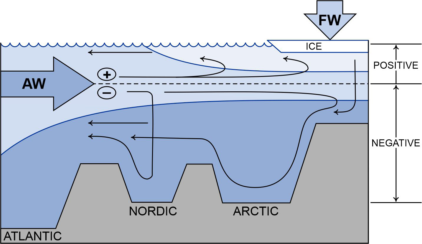
FIGURE 3. Schematic describing the estuary circulation. AW = Atlantic water. FW = freshwater. The sills in Fram Strait between the Arctic Ocean and the Nordic Seas and the Greenland-Scotland Ridge between the Nordic Seas and the North Atlantic are indicated. The plus sign indicates the formation of less dense water and the minus sign the formation of deep overflow water. From Carmack and Wassmann (2006). > High res figure
|
The main part of the Barents Sea inflow enters the deep Nansen Basin along the St. Anna Trough and sinks to and below 1,000 m feeding the deep loop (Schauer et al., 1997). The upper, freshened layer encounters and mixes with water from the Fram Strait branch that enters the St. Anna Trough, and together they form a second boundary stream that flows eastward along the upper part of the continental slope parallel to but inshore of the Fram Strait branch. In the eastern part of the Kara Sea and north of Severnaya Zemlya, the slope narrows and the upper stream moves down slope. The isopycnal mixing with the Fram Strait branch increases and thermohaline intrusions are formed, especially at the core of the Atlantic layer but also in the thermocline above and in the intermediate layers below. The density of the merged stream is high, and it remains in the deep circulation loop.
North of the Laptev Sea, the Atlantic water in the boundary current is then colder and less saline than it is farther west, but it has not lost any appreciable amount of heat (or salt) to the overlying waters. Instead, the colder, less saline upper slope stream, and possibly also other cold, saline contributions from the shelves, mix into the Atlantic layer, reducing its temperature and salinity. The heat has already been lost on the shelves. The Atlantic layer transport increases and its advected heat warms the added water, leading to lower mean temperatures. In recent years, however, Polyakov et al. (2019) have presented evidence that increased wind mixing and weakening stratification in the upper layers may induce increased vertical heat loss.
The water in the boundary current separates from the slope at prominent bathymetric features and enters the deep basins, where it forms gyres and loops that eventually rejoin the boundary current as it leaves the Arctic Ocean through Fram Strait. The water returning from the Nansen Basin is the warmest, while the recirculated water from the Amundsen, Makarov, and Canada Basins has become gradually colder (Figure 4).
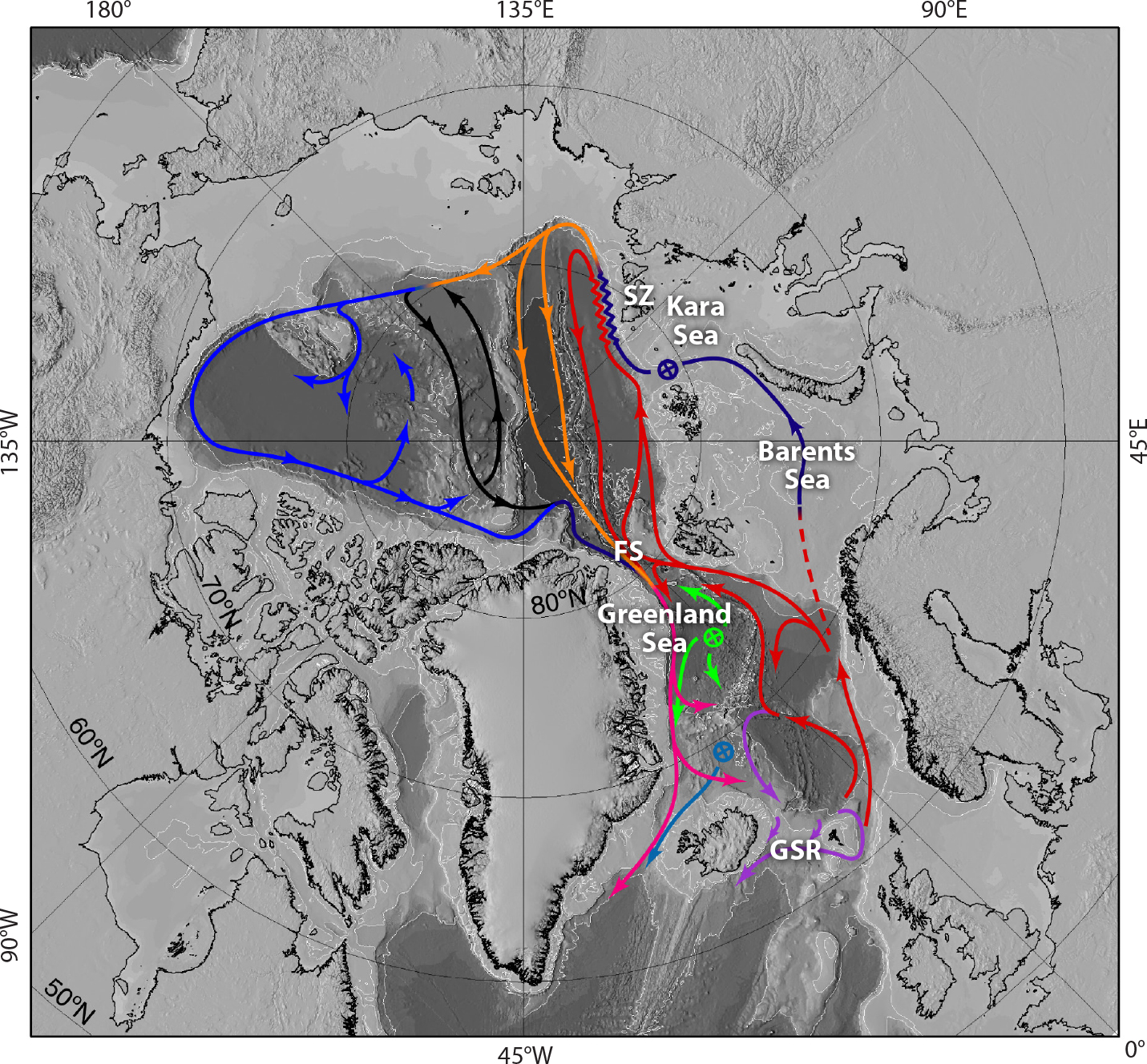
FIGURE 4. Schematic showing the circulation in the subsurface Atlantic Ocean and intermediate layers in the Arctic Ocean and the Nordic Seas. The interactions between the Barents Sea and the Fram Strait (FS) inflow branches north of the Kara Sea and Severnaya Zemlya (SZ) are indicated. The colors of the different loops show the gradual cooling of the Atlantic layer. The recirculation in Fram Strait and the intermediate water formation in the Greenland Sea are shown as well as the overflows across the Greenland-Scotland Ridge (GSR). From Rudels et al. (2012). > High res figure
|
The Norwegian Coastal Current, originating in the Baltic Sea and carrying runoff from there and from the Norwegian coast, moves north in the Norwegian Sea parallel to and shoreward of the Norwegian Atlantic Current and enters the Barents Sea (Figure 1b). Its continuations, the North Cape Current and the Murman Current, bring low salinity water farther along the Eurasian Coast to the Kara and Laptev Seas, where it is augmented by runoff from the large Siberian rivers, Ob, Yenisey, and Lena. In the eastern Laptev Sea this strong, low salinity coastal current splits. One part crosses the shelf break and enters the Amundsen Basin, flooding the boundary current and forming a low salinity layer above the upper layer advected from the Nansen Basin, which now becomes an intermediate water mass, a halocline, above the Atlantic core.
The low salinity shelf outflow directly enters the upper estuarine loop, and the shelf seas farther east, the East Siberian and Chukchi Seas, almost exclusively feed the upper loop. The waters on the shelves are supplied by river runoff and also by a more saline water mass that provides the saline mixing end member. From the Barents Sea to the Laptev Sea, this saline input derives from the Norwegian Coastal Current, while the Chukchi Sea and also the East Siberian Sea receive their saline end members from the Pacific inflow, even though the Pacific is a freshwater source for the Arctic Ocean as a whole.
Although the shelf contributions mainly feed the estuarine loop, they are influenced by the seasonal cycle. In winter, when the runoff is small, dense waters are created by brine rejection and accumulate at the bottom of the shelves to eventually cross the shelf break (Aagaard et al., 1981; see earlier section on Circulation and Stratification). These waters sink as dense boundary plumes that entrain intermediate water until they reach and merge with the basin water column at their appropriate density level. Less dense plumes feed the halocline and may also enter and cool the Atlantic layer. More saline plumes sink through the Atlantic core, entraining and transferring warm Atlantic water downward, adding both heat and salt to the intermediate and deeper layers. While the upper shelf outflows contribute to the estuarine mode, the bypassing plumes strengthen the overturning loop. The volume of entrained water is much larger than the initial volume sinking from the shelves, and the overturning loop becomes denser, more barotropic, and stronger. By contrast, the estuarine loop is only augmented by direct shelf outflow.
Polar Outflow and Double Estuary Exchanges
The export of the less saline upper layer occurs through several passages, the narrow straits in the Canadian Arctic Archipelago and Fram Strait in the East Greenland Current. The outflows have the coast to the right, and their widths are determined by the internal Rossby radius, the ratio of the internal longwave velocity to the Coriolis frequency, here about 10 km (Münchow and Melling, 2008; Rudels, 2010). The main passages are wider than the Rossby radius, and the lower layer reaches the surface in the central part of the straits. Actually, if the density difference is only due to salinity, the relative freshwater excess in the upper layer determines the Rossby radius (Rudels, 2010).
The transport in the boundary currents in each strait can then be estimated from Werenskiold’s expression gΔρH2/2ρf, where g is the acceleration of gravity, Δρ the density difference between the two layers, H the depth of the upper layer at the coast, ρ the reference density, and f the Coriolis parameter (Werenskiold, 1935). If the freshwater input, F, is known, and the entrainment of Atlantic water, MA, is estimated from the turbulent energy input at the surface, Δρ can be determined and the outflow MA + F of upper layer water can be computed (Stigebrandt, 1981; Rudels, 1989).
Spall (2012) adopted a different conceptual approach. He examined marginal seas and applied cooling in the central basin and a geostrophic boundary current bringing heat into the system. Eddy exchanges between the boundary current and the interior balance the heat loss and correspond to the entrainment of Atlantic water into the upper layer in the previous description. The boundary current becomes denser and exits as a deep overflow (Spall, 2012). This picture applies for the Nordic Seas, but Spall (2013) used a similar approach for the Arctic Ocean, where the interactions take place between the boundary current and a freshened upper layer.
The double estuary description implies that the entering water is transformed into both less dense and denser water. Dense water formed in the Arctic Ocean can only exit through Fram Strait, and Rudels (2012) examined the geostrophic exchanges in the strait. He assumed that the upper layer in the Arctic Ocean was created solely by sea ice melting on top of the Atlantic water. If the amount of meltwater and the temperature and salinity of the Atlantic water are known, the distribution of heat loss between the atmosphere and ice melting can be used to determine the amount of Atlantic water transformed into upper layer water when it reaches freezing temperature. This allows for an estimate of the upper layer export in the East Greenland Current. By comparing the two water columns, the East Greenland Current and the Atlantic water in the West Spitsbergen Current, the depth of the pressure reversal below which the Atlantic water enters the Arctic Ocean can then be determined (Rudels, 1989, 2012).
To quantify the deep outflow, some of the created upper layer water was assumed to flow onto the shelves and become transformed by ice formation into brine-enriched, dense water that recrosses the shelf break, sinks down the slope, and entrains Atlantic water. The denser water in the East Greenland Current water column below the upper layer then leads to another pressure reversal, below which the inflow of Atlantic water is arrested and the deep water exits the Arctic Ocean. This approach involves many assumptions about dense water formation on the shelves and entrainment at the slope that are elaborated further in Rudels (2012).
One finding is that no baroclinic balance between the inflows and outflows can be established. If only the estuarine circulation is present, the inflow below the pressure reversal can only be stopped by a sea level slope and a barotropic pressure head directed out of the Arctic Ocean. In the case of a double estuary, the deep outflow cannot be arrested and sea level decreases in the Arctic Ocean, which generates a balancing barotropic inflow in the West Spitsbergen Current. Another possibility would be a still denser water mass in the Nordic Seas that creates a further deep pressure reversal. Only if the deepest pressure reversal is close to sill depth would the baroclinic exchanges approximately balance. Mass (volume) balance in the Arctic Ocean should be established within months, but the baroclinic freshwater exchange might take years to reach a balance between input and outflow—and perhaps a balance is never achieved.
One interesting question concerns whether or not a double estuary circulation could be created in an Arctic Ocean with shelves and heat loss but with no freshwater input. Ice formation on the shelves would lead to brine rejection, dense water formation, and slope convection, thus sustaining the overturning loop. The ice would melt partially by solar radiation in summer and by heat entrained from Atlantic water below in winter, and a less dense upper layer would form, establishing the upper estuarine part of circulation. Freshwater input would then not be needed.
Double estuary circulation has been further elaborated in conceptual models by, for example, Lambert et al. (2016) and Haine (2021). These models ignore, as do most conceptual models and also the approach presented here, the inflow over the Barents Sea. The Barents Sea inflow is largely barotropic and mainly forced by wind and sea level slope and cannot easily be incorporated in the baroclinic description used for double estuary exchanges through Fram Strait.
Freshwater Storage and Upper Layer Circulation
The least saline upper layer is found in the Amerasian Basin, and in particular in the Beaufort Gyre, where the water column stores more than 20 m of freshwater (relative to 34.80). This accumulation of freshwater is attributed to the clockwise atmospheric circulation over the Beaufort Sea that drives Ekman transports toward the center of the gyre, creating a deep bowl of low salinity water. Such accumulation cannot go on indefinitely, and the deeper part of the bowl becomes baroclinically unstable and sheds eddies into the surrounding waters. Model studies by Manucharyan and Spall (2016) indicate that these two processes should balance when the freshwater storage in the gyre reaches around 34 m. This is, however, much more than observed, suggesting that not all processes are taken into account.
There is another mechanism that can reduce the freshwater accumulation. As the gyre is spun up by the wind, the concentration of low salinity water at the center creates a density distribution that generates a clockwise geostrophic flow, but in summer, when the winds are weaker, the atmospheric forcing of the ice almost disappears. Instead, the ice cover retards, by friction, the underlying geostrophic circulation and flattens the isopycnals. This process adds to the eddy shedding in limiting the freshwater accumulation and should keep it around the 20 m that is presently observed (Meneghello et al., 2018). However, if, in a warming climate, the ice cover decreases in thickness and compactness, its braking capability is reduced, which allows for more freshwater storage in the Beaufort Gyre (Doddridge et al., 2019).
The liquid freshwater content in the Arctic Ocean has increased from 93,000 km3 during the last two decades of the twentieth century to 101,000 km3 during the first decade of the twenty-first century. At the same time, the sea ice volume has decreased from 17,800 km3 to 14,300 km3, providing about two-thirds of the freshwater input. Almost all of this freshwater increase is concentrated in the Beaufort Gyre, from 18,500 km3 to 23,500 km3 (Haine et al., 2015). Superficially it appears as if the sea ice meltwater added to the upper layer has been concentrated in the Beaufort Gyre.
Proshutinsky et al. (2019) analyzed different sources that contributed to freshwater storage in the Beaufort Gyre between 2003 and 2018 and found that the largest input, 15% to 45%, came from the Mackenzie River, but it was strongly dependent on atmospheric forcing. A clockwise circulation draws the water into the gyre, while an anticlockwise circulation carries the Mackenzie runoff directly to the Canadian Arctic Archipelago. The Bering Strait inflow could contribute between 5% and 50%, again depending on the year, while melting of sea ice and downward Ekman pumping of sea ice meltwater in the center of the gyre contribute between 10% and 20% of the freshwater anomaly. Low salinity waters derived from the Eurasian shelves are also found in the Beaufort Gyre, but the input depends upon the wind field. When the clockwise circulation is weak over the Amerasian Basin and the anticlockwise circulation is strong over the Eurasian Basin, the anticlockwise gyre in the Eurasian Basin expands into the Makarov Basin, and some of its water is drawn into the Beaufort Gyre (Morison et al., 2012). The main conclusion, however, is that the present large freshwater storage in the Beaufort Gyre is due to a persistent clockwise atmospheric circulation that has forced the upper low salinity layers toward the gyre.
Internal Mixing Processes
Wind and the seasonal heating and cooling cycle are the main external forcings on the Arctic Ocean. In winter, the upper layer is homogenized by ice formation and brine rejection, and wind stress reaches down to the strong permanent halocline. In summer, sea ice melting creates a low salinity meltwater layer that inhibits deep wind mixing in spite of more open water and more mobile ice floes leading to stronger stirring. Some solar radiation penetrates below the meltwater layer and creates a near-surface temperature maximum that might, or might not, survive the deepening of the Polar Mixed Layer the following winter (Jackson et al., 2010).
The deep interior of the Arctic Ocean is shielded from surface forcing by its strong stability, but mixing processes using other energy sources may be important in the deeper layers. Tidal motions affect the entire water column, but when they interact with bottom topography, both well-mixed turbulent bottom layers and internal tides are generated. The Arctic Ocean is largely located north of the critical latitude (75°N) where the inertial period is shorter than the M2 tidal period. Internal tides then cannot propagate but instead dissipate their energy where they are created, especially above the continental slopes (Rippeth et al., 2015).
Another internal process is double-diffusive convection, where, if one component, heat or salt, is unstably stratified, the potential energy stored in the unstable density distribution can be released by the more rapid molecular diffusion of heat. An unstable stratification in salinity, saline water above fresh, is uncommon in the Arctic Ocean, while, as a β ocean, an unstable distribution of temperature, cold water over warm, is the norm in the upper layers above the Atlantic temperature maximum. This leads to formation of diffusive interfaces. Heat diffuses through the interfaces, generating unstable layers, warm above and cold below the interface, that eventually grow unstable and convect, homogenizing the layers above and below. This diffusive-convective process creates thermohaline staircases that are especially prominent in the deep thermocline above the Atlantic layer in the Canada Basin (Neal et al., 1969) but are also present in the other basins.
Double-diffusive convection is primarily a vertically driven process, but it can induce lateral exchanges between water masses through thermohaline intrusions, which are observed almost everywhere in the Arctic Ocean. The classical theory for intrusion formation (Stern, 1967) requires that one component is unstably stratified and that lateral, density-compensating gradients of both heat and salt are present. Small disturbances will grow when salt is unstably stratified, and the perturbations are such that warm intrusions rise and cold intrusions sink across the front. If heat is unstably stratified, rising cold and sinking warm intrusions will grow. A warm intrusion has a diffusive interface above and a salt finger interface below, while the situation is reversed for a cold intrusion. The motions are driven by the differences in density fluxes through the two interfaces. Thermohaline intrusions in the Arctic Ocean are, however, observed in almost all types of stratification, and also when both components are stably stratified and where the classical approach does not apply. They are less frequent and less developed when the background stratification is in the salt finger sense, which was the situation examined by Stern.
Thermohaline intrusions, and also individual eddies, are generated at and spreading from narrow fronts between water columns with different properties. The strongest front in the Arctic Ocean is located above the Kara Sea slope between the warm, saline Fram Strait branch and the colder, fresher Barents Sea branch (Figure 5). Intrusions there are observed in the diffusively unstable part above the temperature maximum, in the stable-stable range between the temperature and salinity maxima, and also below the salinity maximum, where they are most strongly developed in the stable-stable part below the intermediate salinity minimum.
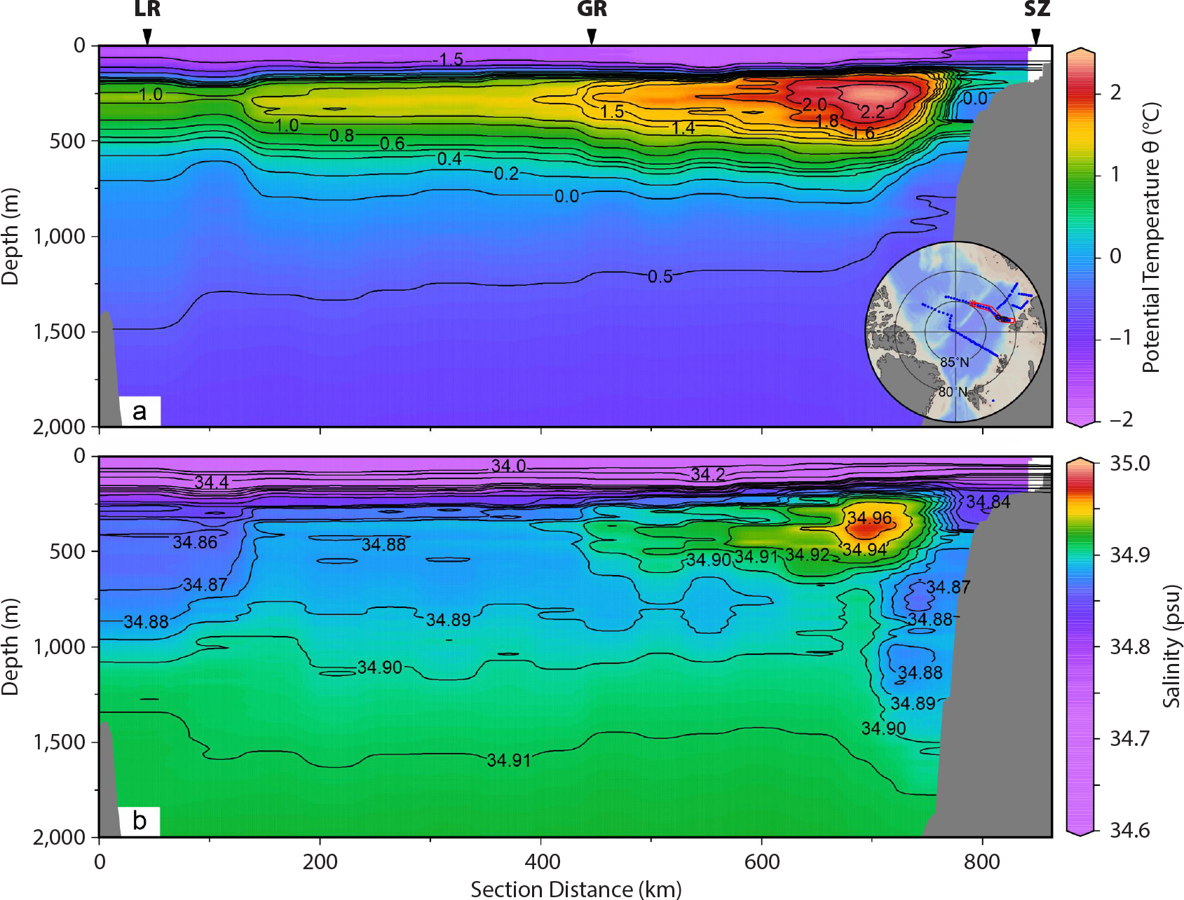
FIGURE 5. Potential temperature (a) and salinity (b) sections across the Nansen Basin from Severnaya Zemlya (SZ) over the Gakkel Ridge (GR) to the Lomonosov Ridge (LR) (the section position is indicated on the (a) inset) showing the cold, less saline Barents Sea branch entering the Nansen Basin at the continental slope and the presence of Barents Sea branch water over Gakkel Ridge and in the Amundsen Basin. Thermohaline intrusions are present between the warm, saline Fram Strait branch and the Barents Sea branch at the slope and in the interior of the Nansen Basin (observations from Polarstern 2011). > High res figure
|
When both components are stably stratified, finite lateral disturbances are needed to create initial inversions that eventually evolve into diffusive and salt finger interfaces. Such disturbances could be created by internal tides that carry waters across the front. However, intrusions are also found on the basin side of the Fram Strait branch (Figure 5). This raises the question of the importance of intrusions in spreading heat from the Atlantic water at the boundary to the interior of the basins. One view is that the intrusions grow laterally and reach well into the center of the basins (Walsh and Carmack, 2003). A second view assumes that the expansion of the intrusions is limited to the frontal zone. After the potential energy stored in the unstably stratified component is removed, the intrusions are advected as relicts with the main circulation (Rudels et al., 1994; Rudels and Hainbucher, 2020).
The intermediate waters on the basin side of the Fram Strait branch have characteristics that can only derive from the Barents Sea inflow branch at the Kara Sea slope. This implies that the water entering the boundary current from the Kara Sea shelf must move into the basin from the Laptev Sea slope farther east. The Barents Sea branch is located on the slope side of the Fram Strait branch, suggesting that substantial fractions of the two inflow branches as well as the intrusions created between the branches also leave the slope and move toward Fram Strait within the Nansen Basin (Figures 4 and 5).
There is a possible connection between thermohaline staircases and thermohaline intrusions. Transports through the interfaces are commonly taken to depend upon the magnitude of the unstable density step, αΔT or βΔS, raised to the 4/3 power (Turner, 1973). An intrusion created in the thermocline above the temperature maximum has an unstable temperature step αΔT at the diffusive interface that is larger than the corresponding unstable salinity step βΔS at the salt finger interface. This leads to stronger density transport across the diffusive interface, and the stabilizing temperature step at the salt finger interface is eventually removed. The more saline upper and the less saline lower layers then merge, transforming the intrusive layers into a thermohaline staircase with thick homogeneous layers and small stability ratios (Rudels, 2021).
Such thick layers have been observed at the Laptev Sea slope and in the Eurasian Basin (Polyakov et al., 2012b, 2019). These staircases could transfer heat from the Atlantic water to the surface layer and the ice cover in the Nansen Basin. In the other basins, especially the Canada Basin, where the staircases have high stability ratios, such transfer is less likely. The fluxes there are smaller, and the thermocline lies below the temperature minimum created by the inflow of Bering Strait winter water, which prevents further vertical transfer of the heat.
The nonlinearity of the equation of state for seawater induces other effects. Cabbeling, or contraction on mixing (Witte, 1902; Foster, 1972), causes the mixture of two waters with different temperatures and salinities to become denser than the initial waters. Smith et al. (1937), suggested that cabbeling could be important in the formation of the intermediate layers in the Labrador Sea by lateral mixing between waters from the rim and from the central core. However, the nonlinearity decreases with increasing temperature, salinity, and pressure, and the contraction is less in the deeper layers. Furthermore, the density increase does not take place before the mixing is complete down to the molecular level, which requires strong turbulent stirring to rapidly reach the appropriate mixing length scale (Eckart, 1948), which likely limits its importance. Molecular mixing and diffusion rather suggest that cabbeling should be considered as a perturbation on double-diffusive convection, making the density fluxes into the colder water above less intense than those into the warmer water below the interfaces, causing the interface to move upward (McDougall, 1981a, b).
Another nonlinear feature is that cold water is more compressible than warm—the thermobaric effect. This implies that an externally forced downward displacement in a weakly stratified water column with unstable temperature but stable salinity distribution might grow and convect. In contrast to double-diffusive convection and cabbeling, the thermobaric effect does not require mixing to be triggered, and once it has passed the critical density threshold it would continue to sink (Gill, 1973). It is also asymmetric: cold water might be induced to sink, but warm water will not rise.
The thermobaric effect also affects lateral mixing between water masses (John Shepard, pers. comm., 1979), especially between a boundary current and the basin interior. If the isopycnals slope upward from the coast, as is the case of a warm buoyant boundary current (Atlantic inflow), the exchange trajectories between the boundary current and the interior will not be along but rather below the isopycnals, spreading the boundary current downward. In the case of a cold, less saline boundary current with isopycnals sloping upward from the coast (polar outflow), the exchanges between the boundary and the interior will take place above the isopycnals, concentrating and confining the boundary current to the surface. If the isopycnals slope downward from the boundary, as is the case for a deep, cold overflow, the exchange trajectories are again below the isopycnals and the boundary current spreads downward. Aagaard et al. (1985) noticed that the outflow of warmer Arctic Ocean deep water in the East Greenland Current was located around 2,000 m above the colder Greenland Sea deep water and attributed this to the thermobaric effect.
Outlook
As noted in the introduction, Quadfasel et al.’s (1991) observations of Arctic warming three decades ago altered our perception of the Arctic Ocean, from being a place in steady state to one that is highly variable. They expressed the urgent need to understand this system under a rapidly changing climate. Indeed, today the persistent loss of sea ice has become the leading signal of global warming, and few current papers fail to mention that the Arctic is warming two to three or more times faster than the rest of the planet. Our effort in this paper has been to emphasize the structure of the Arctic Ocean and the key mechanisms that determine that structure. In our opinion, two questions are clear in looking to the coming three decades: (1) How will the structures, functions, and fluxes of the interior ocean respond to climate forcing? (2) How will biogeochemical systems respond to an Arctic Ocean in transition?
As a β ocean, there are few physical processes and biogeochemical functions that are not constrained by the regionality and seasonality of freshwater supply, disposition, storage, phase, and export to the global ocean (Carmack et al., 2016). In the coming years, the hydrological cycle of poleward freshwater transport is expected to increase, and this would result in stronger stratification and reduced vertical fluxes of heat and material properties. System-wide complex interactions, however, make predictions difficult. In terms of supply, for example, quantification of river inputs will require better estimates of trans-evaporation, lake effects, and permafrost thaw within surrounding drainage basins. The freshwater phase (i.e., solid, liquid, or vapor) will depend on the global rate of climate warming and interactive air-ice-sea heat exchanges. The future of freshwater disposition, storage, and export will respond to new patterns of wind forcing and coupling as the ice cover progressively retreats in summer. Responses will definitely be spatially heterogeneous, as for example are the opposite responses of the Eurasian and Amerasian Basins to climate forcing thus far (Polyakov, 2020). Seasonal signals are strengthened; the area of seasonal melting and freezing is already growing, currently increasing the seasonal burden of freshwater in the summer mixed layer. Later, however, the seasonal melt rate might decrease as the Arctic Ocean grows more ice-free year-round (Brown et al., 2020). In the long run, the control of export relative to storage, the systemwide freshwater residence time, will determine whether the Arctic will freshen or not, and much remains uncertain.
Other scenarios exist. While a warmer climate could increase the freshwater input and strengthen the upper loop, a warmer Atlantic water might lead to a larger fraction of oceanic heat going to ice melting, increasing the stability between the upper and the Atlantic layer, reducing entrainment from below, and weakening the upper estuarine circulation. This reduction might be stronger than the increase due to larger runoff. At the same time, the salinity on the shelves becomes lower and the production of saline shelf water diminishes, leading to a weakening of the overturning loop. A warmer climate would then result in an overall weaker double-estuary circulation.
One part of the double-estuary circulation that has already diminished is the deep and bottom water formation in the Greenland Sea. The deepest layers are no longer renewed by local convection, but by advection of deep waters from the Eurasian and Amerasian Basins. The water now formed in the Greenland Sea is Arctic intermediate water, less dense than the Amerasian Basin deep water. Hence, the thermohaline roles of the Greenland Sea and the Arctic Ocean have changed (Marnela et al., 2016). The Greenland Sea no longer forms the densest water in the Arctic Ocean-Greenland Sea system, but it might now provide the densest component of the overflow water to the North Atlantic.
Biogeochemical systems will respond in multiple ways to a changing physical environment, but three questions are germane: (1) Will new production increase or decrease? (2) Will acidification threaten marine organisms? (3) Will northward spreading waters and organisms from subarctic seas displace existing ecosystems? With regard to the first, the Arctic Ocean is decidedly an oligotrophic system. The balance is between increasing light input owing to sea ice retreat and decreasing nutrient supply owing to increased salt and heat stratification. The two mechanisms also interact, as ice retreat beyond the shelf break will increase upwelling of nutrient-rich waters, while increased nutrient supply may result in self-shading and reduced light availability. Acidification is typically reported in terms of aragonite undersaturation (omega) values, and the central Canada Basin was the first deep ocean region in which omega fell below its critical value, making the waters corrosive (Yamamoto et al., 2009). Introduction of new species by advection from subarctic waters or invasion due to changing environmental conditions will impact the food web through complex, cascading mechanisms.
Quadfasel et al.’s observations were a wake-up call. But, as recalled by Aagaard and Carmack (1989), the message of change was preached almost a century earlier by Fridtjof Nansen himself: he ended a lecture on the Fram drift, delivered in 1897, with these words: “Everything is drifting, the whole ocean moves ceaselessly, a link in Nature’s never-ending cycle, just as shifting and transitory as the human theories.” Would Nansen judge us ready for the future?
Further Reading
The presentation of the processes and circulation of the Arctic Ocean given here represents our personal views and reflections. It is drawn with broad brushes, and the number of references is kept low. Other recent summaries of the Arctic Ocean circulation that include many relevant references and discussions are Bluhm et al. (2015, 2020), Rudels (2019, 2021), Wassmann et al. (2020), Timmermans and Marshall (2020), and Lenn et al. (2021).
Acknowledgments
We want to thank Patricia Kimber for her help with the figures. Figures 2 and 5 were made using Ocean Data View (Schlitzer, 2017). We also thank two anonymous reviewers for their questions, advice, and interest.