Background
The primary motivations today for ocean monitoring are to determine the ocean’s role in climate and climate change, and to quantify and understand ocean variability and trends in heat, freshwater, and carbon (and other biogeochemical) fluxes, as well as the impacts of such changes on other ecosystem-relevant parameters. We focus here on the Arctic Ocean, a relatively small body of water that is important for the global heat balance, and that is observed to be warming faster than the global mean rate as a consequence of regional feedbacks. We also include the Nordic Seas, a key buffer zone or transitional basin between the subpolar North Atlantic and the Arctic Ocean, where much of the regional dense water formation—via surface heat loss—occurs. The Arctic Ocean is unusual. It only comprises ~3% of the global ocean surface area, but it receives >10% of global river runoff; it is >50% (by area) relatively shallow shelf seas, the rest is deep ocean; and it is largely surrounded by land (Jakobsson, 2002; Carmack et al., 2016).
The regional geography—the confinement of the Arctic Ocean and Nordic Seas by land—is what makes ocean boundary monitoring feasible (Figure 1). The Arctic Ocean connects to adjacent basins through narrow and/or shallow gateways: to the Pacific through Bering Strait, to the subpolar North Atlantic through Davis Strait, and to the Nordic Seas through the Barents Sea Opening and Fram Strait. Of these four, only Fram Strait is deep. The Nordic Seas connect to the subpolar North Atlantic across the relatively wide and shallow Greenland-Iceland-Scotland (GIS) Ridge. We note also the existence of one other exit from the Arctic Ocean. Fury and Hecla Strait separates the Canadian mainland from Baffin Island and may support a net throughflow from the Arctic Ocean, through the Canadian Arctic Archipelago, then on into Foxe Basin (north of Hudson Bay), and ultimately into the Labrador Sea via Hudson Strait. However, as Tsubouchi et al. (2012) argue, any such throughflow will be small, and presently available measurements indicate its mean to be smaller than its uncertainty.
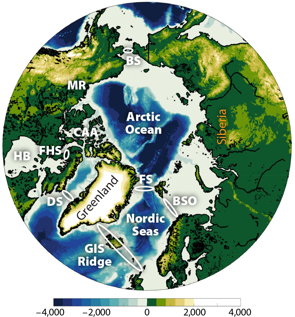
FIGURE 1. This regional map of the Arctic Ocean and Nordic Seas shows depths/elevations in meters (see scale). BS = Bering Strait. MR = MacKenzie River. CAA = Canadian Arctic Archipelago. FHS = Fury and Hecla Strait. HB = Hudson Bay. DS = Davis Strait. GIS = Greenland-Iceland-Scotland Ridge. BSO = Barents Sea Opening. FS = Fram Strait. > High res figure
|
Arctic Ocean boundary measurements allow calculation of ocean exchanges with adjacent basins and also air-sea fluxes. A closed circuit of measurements (which may or may not include coastline) defines a volume, enabling the application of inverse methods, developed in the ocean context in the 1970s from earlier seismology applications (see Wunsch, 1996). Inverse methods generate allowable, self-consistent adjustments to current velocities (and other parameters) within uncertainties, to conform to constraints—at a minimum, mass and salt conservation—without which, unaccounted residuals mean that net surface fluxes (of heat and freshwater) cannot be meaningfully calculated. As current measurements became more widely available, their incorporation into inversions increased the usefulness of the approach by better initialization and narrowed uncertainty range. Calculation of property divergences within the defined volume is then facilitated by the mass-balanced boundary velocity field, as demonstrated by Bryan (1962) for ocean heat fluxes in a single-section context, and widely extended thereafter. The principle is straightforward: in the Arctic Ocean, mainly warm and saline seawater enters, and cooled and freshened seawater and sea ice leave. The amount of heat and freshwater required to effect these transformations is then the relevant surface fluxes.
The ability to calculate year-round property divergences within the Arctic Ocean from boundary measurements is useful because the Arctic is still data sparse, particularly for the deep ocean and the atmosphere and during winter–spring (November–May; see Behrendt et al., 2018). The regional lack of data is well illustrated by Cowtan and Way (2014, their Figure 1), who note that the different approaches taken to redress the deficiency all have limitations: extrapolation spreads out the (limited) available information, reanalyses essentially infill with dynamics, and remote-sensed (satellite microwave sounding) measurements are weighted to the lower troposphere and not the surface. While these resources are all valuable, ocean boundary measurements have the potential to provide independent, integral (regional) constraints on surface fluxes.
Data on heat exchanges between the atmosphere and the ice and upper ocean—derived from ocean boundary measurements—are now beginning to be used to better quantify and assess regional climate system parameters. Similarly, knowledge about total continental river runoff, which typically accounts for around one-third of the total runoff, is limited by the problem of ungauged rivers. There are several different approaches to addressing this limitation. Ocean surface freshwater fluxes derived from ocean boundary measurements are the sum total of evaporation, precipitation, and runoff, and may usefully constrain estimates of total runoff.
Net exchanges require simultaneous knowledge of all inflows and outflows, so here we confine ourselves to publications using mass-balanced ice and ocean velocity fields around the entire Arctic Ocean boundary, which are all derived using inverse methods. This review is structured as follows. The next section provides a brief overview of methods, focusing on recent developments. It is followed by sections describing computed surface heat and freshwater fluxes, physical oceanographic outcomes that examine water mass transformation rates, and the use of mass-balanced boundary velocity fields to compute net fluxes of biogeochemical quantities. We conclude with a summary and offer perspectives and comments relevant to this discussion.
Methods
We do not further describe the application of inverse methods, which Wunsch (1996) thoroughly covers. Rather, we focus here on progress over the last 10 years in the calculation and interpretation of ocean (and sea ice) freshwater fluxes and heat fluxes.
Aagaard and Carmack (1989) first demonstrated the possibility of generating Arctic freshwater budgets and introduced “direct” and “indirect” methods. The former summed estimates of evaporation, precipitation, and runoff for a total of ~0.2 Sv (1 Sv = 106 m3 s–1), and the latter used ice and ocean budgets, ~0.1 Sv. The direct estimate proved to be quite robust, and improvements in ice and ocean measurements brought indirect estimates reasonably into line.
However, conventional calculation of ocean freshwater fluxes requires salinity “reference values,” the choice of which has been plagued by arbitrariness, where authors typically justify their choices verbally, while a physically and mathematically consistent approach has been lacking. The ocean is ~96.5% freshwater, so how then to identify a particular fraction as somehow “different”? Development of a closed and complete method to quantify ocean freshwater fluxes was initiated in Tsubouchi et al. (2012) and extended by Bacon et al. (2015). This method begins with the observation that there is one location in the ocean where a true freshwater flux occurs unambiguously: the surface, where freshwater is exchanged with the atmosphere via precipitation and evaporation, and where the ocean receives freshwater from the land via river runoff, which is taken to include terrestrial glacial discharge. The outcome is an equation that expresses total surface freshwater flux, within an ocean volume enclosed by measurements (and coastline), as the sum of three terms: (1) the divergence of the salt flux around the ocean volume’s boundary, (2) the change in total (ice and ocean) seawater mass within the ocean volume, and (3) the change in mass of salt within the ocean volume. Term (1) expresses the dilution of the (mainly saline) inflows by the surface freshwater flux to form the (freshened) outflows, and is also the steady-state solution, where seawater mass and its salt content are invariant. Terms (2) and (3) combine to isolate the net freshwater mass change in the full, time-varying solution. A scaling term emerges from the mathematics that resembles the traditional reference salinity, but it is the ocean volume’s ice and ocean boundary-mean salinity. This may not, however, be the last word on the subject; for a critical review, see Solomon et al. (2021).
Bacon et al. (2015) apply the same approach to the (ice and ocean) surface heat flux as an exchange between ocean and atmosphere. It does not achieve a similarly closed form, because the transport by the (very small) boundary mean ocean velocity of the boundary mean temperature remains, which is unsatisfactory because it depends on the temperature scale.
Tsubouchi et al. (2012) provide an algebraic form and demonstrations of the impact on freshwater flux calculations of variant reference salinity choices. Within a closed circuit of measurements, the surface freshwater flux is only weakly sensitive (to ~1%–2%) to choice of reference salinity. However, when considering open hydrographic sections with a non-zero net mass budget, differences can be substantial—tens of mSv in volume terms, for changes of order 0.1 g kg–1 salinity. Furthermore, oceanographers wishing to calculate freshwater fluxes should consider not only how to do it but also what the computed flux means. As Carmack et al. (2016) illustrate, for the Arctic, the simplest case is that the surface freshwater flux dilutes all of the inflows to become all of the outflows. By considering the boundary gateways separately, the approach quantifies how the surface freshwater flux and the relatively fresh Bering Strait inflow combine to dilute (some of) the inflowing Atlantic-origin waters to become the outflows.
Budget approaches make no distinction between types of water molecules. However, evaporation and freezing act as distillation processes. Evaporation preferentially removes isotopically lighter (via oxygen) water molecules, which return in consequent precipitation and runoff. Freezing similarly produces isotopically lighter sea ice while rejecting heavier brine (high-salinity seawater with a higher proportion of the heavier isotopes). These characteristics are conservative and are distinctly separate in the phase space of salinity and the oxygen isotope (via its anomaly). Forryan et al. (2019) used a standard method to identify source fractions of seawater, meteoric freshwater, and sea ice/brine, which they then combined with boundary velocities to calculate transports. Within uncertainties, the oceanic meteoric freshwater flux (implicitly including runoff) was indistinguishable from the surface freshwater flux (as the total of precipitation minus evaporation plus runoff), reinforcing the robustness of both methods.
Surface Heat and Freshwater Fluxes
Tsubouchi et al. (2012) calculated the first quasi-synoptic estimates of pan-Arctic surface heat and freshwater fluxes. They assembled sea ice and hydrographic section data around the boundary of the Arctic Ocean from a 32-day period in summer 2005 and applied inverse methods to generate a mass- and salinity-balanced boundary velocity field. Their resulting net heat and freshwater fluxes were ~190 TW (from ocean to atmosphere) and ~190 mSv (into the ocean), respectively.
Tsubouchi et al. (2018) repeated the procedure, calculating a piecewise-continuous single annual cycle (from September 2005 to August 2006) of fluxes at monthly resolution, based synoptically on moored measurements. These first (almost) entirely measurement-based estimates of annual mean (±std) surface heat and freshwater fluxes are 175 ± 48 TW (15.5 ± 4.2 W m–2) and 204 ± 85 mSv (6,400 ± 2,700 km3 yr–1), and the calculations include contributions of 22 ± 15 TW and 48 ± 32 mSv from sea ice. Their boundary heat flux variability through the year derives mainly from Atlantic water velocity variability and from surface water temperature variability, while the boundary freshwater flux variability is dominated by Bering Strait velocity variability. They inspect various published reanalyses, which give Arctic surface heat fluxes ranging from 5 W m–2 to 19 W m–2, so that those at the lower end may appear questionable. They also note that their surface freshwater flux agrees with that of Haine et al. (2015), 6,770 km3 yr–1.
Tsubouchi et al. (2018) explain their neglect of storage as follows. Heat and freshwater storage are approximated as the sums of two components: repeating seasonal cycles of zero mean, and long-term trends (see Armitage et al., 2016). The annual averages of the ice and ocean boundary fluxes then accurately represent the annual averages of the surface fluxes, when the long-term trends are included as relatively small contributions to their uncertainties. They say “accurately represent” rather than “are equal to” because the ice and ocean boundary fluxes are the result of a complex convolution of the trajectories of individual water parcels with the action of surface fluxes upon them over many years, except at Fram Strait, where some of the northbound waters in the east of the strait may recirculate and only spend weeks to months inside the region before leaving southward in the west of the strait. Long residence times mean that seasonal heat and freshwater cycles (warming/cooling and melting/freezing) are local (i.e., largely confined within the boundary). Bacon et al. (2015) illustrate the consequent smoothing of surface fluxes using model output. The seasonal cycle amplitudes of surface and boundary heat fluxes are notably different, ~500 TW versus ~50 TW (or roughly 50 W m–2 and 5 W m–2), respectively. The two freshwater seasonal cycles are more similar because some of the signal is a phase change with little net mass change.
Mayer et al. (2019) present the most cogent analysis of the Arctic climate system heat budget to date. A suite of largely independent observational and reanalysis products defines the atmosphere, sea ice, and ocean. They employ the same Arctic Ocean boundary measurement resources as Tsubouchi et al. (2018), but for four years (2005–2009), because they deem in situ-based oceanic transports to be more reliable than those from reanalyses. Budget closure is enforced per calendar month using a variational method. Focusing on their ice and ocean results, they find an annual mean surface heat flux of 16 W m–2 (ocean to atmosphere), with seasonal extrema in January (60 W m–2, ocean to atmosphere) and July (94 W m–2, atmosphere to ocean). They also estimate heat accumulation in the Arctic using a longer time base (2001–2017), indicating that the energy imbalance of the Arctic Ocean domain is ~1 W m–2, with two-thirds going into seawater warming and one-third going into sea ice melting. Their analysis also identifies that, for the Arctic seasonal cycle, the largest source of uncertainty is sea ice thickness, because reanalyses only assimilate concentration. Furthermore, the ocean measurements show oceanic heat transports in ocean reanalyses to be too weak. Mayer et al. (2019) clearly demonstrate the value of measurement-based ocean flux estimates independent from other data products, as does the recent analysis of Arctic riverine discharges by Winkelbauer et al. (2022). Such estimates are used both to constrain choices of other data resources and are key to final quantified results. Mayer et al. (2019) note that ocean boundary measurements offer a “unique opportunity for long-term monitoring of the coupled Arctic energy budget.”
Tsubouchi et al. (2021) extend the geographical range of northern high-latitude ocean heat flux estimation down to the region of the GIS Ridge. They employ a hybrid data set in which the main resources describing the Atlantic water inflows span the years 1993–2016 at monthly resolution. These critical measurements contain the bulk of the ocean heat transport variability. Some of the ocean transport records are shorter so, to obtain continuous monthly transport time series over the entire period, short time series were extended using the average value of the record modulated by its mean seasonal cycle. Inverse methods were applied to obtain closed budgets between the GIS Ridge, Davis Strait, and Bering Strait. They find that the mean ocean-to-atmosphere heat flux was 305 ± 26 TW, and that a statistically significant increase of 21 TW occurred within the period, after 2001. Using other published heat flux estimates (including Tsubouchi et al., 2018), they infer the heat flux over the Nordic Seas (excluding the Barents Sea) to have been 137 ± 34 TW.
Interior Mixing and Net Vertical Exchanges
The net water mass transformation exerted by the Arctic is to cool and freshen relatively warm, saline Atlantic-sourced waters that enter through eastern Fram Strait and the Barents Sea Opening and return southward east and west of Greenland via western Fram Strait and Davis Strait. Tsubouchi et al. (2018) calculate net (annual mean) freshening (by ~0.6 in salinity) and cooling (by ~3.7°C), for a density reduction of ~0.2 kg m–3, not much different from the equivalent values for summertime from Tsubouchi et al. (2012). Some water returns denser than it entered, and some lighter, a twofold process that was first described as a double estuarine circulation by Carmack and Wassmann (2006). Brown (2019) quantifies this “two-cell” (double estuarine) vertical circulation in the Arctic Ocean in the first study derived from measurements.
To calculate density budgets for each isopycnal layer and thus infer the diapycnal mixing rates needed to maintain Arctic stratification, Brown (2019) uses the formulation of Walin (1982), adapted for density transformations by Large and Nurser (2001), whereby advective fluxes of density are taken to be balanced by density fluxes at the surface and by turbulent diffusion of density in the interior. The Tsubouchi et al. (2012) estimates of Arctic Ocean boundary velocities and density fields are used, with surface flux data from atmospheric reanalyses. Climatologies are employed to estimate total monthly river runoff and to define areas of surface flux integration.
The principal finding of Brown (2019) is that the inflowing Atlantic waters are indeed split, with portions transformed into both lighter and denser waters, confirming the existence of an overturning circulation with both an upper and a lower cell. Densification is due to surface heat loss and is concentrated in the southwestern part of the Barents Sea where warm Atlantic waters enter the region. In the lower cell, 1.8 Sv of inflowing Atlantic waters become more dense through surface heat loss; diapycnal mixing plays a secondary role here. Buoyancy gain, on the other hand, results from net freshwater input to the Siberian shelves and also offshore of the Mackenzie River outflow. In the upper cell, 1.0 Sv of Atlantic waters are transformed into lighter waters through mixing with surface-freshened water classes. These waters still lose heat to the atmosphere, but the upward flux of density is dominated by turbulence.
The density budget requires a positive upward diffusive density flux, equivalent to (pan-Arctic) diffusivities throughout the water column of ~1 × 10⁻⁵ m2 s–1, decreasing to ~1 × 10⁻⁶ m2 s–1 toward the surface. Therefore, in contrast to some previous studies, Brown (2019) finds that in the Arctic Ocean, diffusive fluxes due to subsurface diapycnal mixing play as significant a role as surface buoyancy fluxes in controlling water mass transformations. Figure 2 illustrates the two-cell overturning results in density terms.
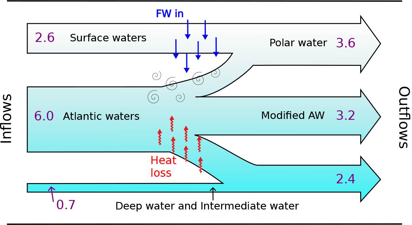
FIGURE 2. Schematic of the Arctic Ocean two-cell overturning in density space. Heat loss and freshwater (FW) input occur at the surface. Volume transports at entry and exit are shown in Sv. Interior diapycnal transports out of the Atlantic waters are 1.8 Sv dense waters downward and 1.0 Sv lighter waters upward. > High res figure
|
As first observed by Mauritzen (1996), water mass densification by surface heat loss in the Nordic Seas is largely responsible for the conversion of Atlantic waters into the dense, intermediate-depth water masses that overflow the GIS Ridge and descend to form headwaters of the Atlantic Meridional Overturning Circulation (AMOC; Frajka-Williams et al., 2019). Given a temperature difference of 8.4°C and an overflow volume transport of 5.5 ± 0.3 Sv, Tsubouchi et al. (2021) state a required heat loss of 189 ± 14 TW for this densification. Assuming that all of the heat loss is used to form the overflows, the 137 TW heat loss in the Nordic Seas can create 4.0 Sv of overflow waters, which also implies that the remainder of the densification, equivalent to 1.5 Sv, must happen in the Arctic Ocean (including the Barents Sea).
Overall (and approximately), therefore, 9 Sv of seawater enter the domain of the Nordic Seas and the Arctic Ocean, comprised of 1 Sv Pacific and 8 Sv Atlantic waters. One Sverdrup of the Atlantic water is transformed in the Arctic Ocean into lighter waters, to supplement the 1 Sv cold and fresh Pacific water, leading to 2 Sv exported in the upper cell. Four Sverdrups are made denser in the Nordic Seas and 1.5 Sv in the Arctic Ocean, to be exported in the lower cell as GIS Ridge overflow waters (see Isachsen et al., 2007). This leaves perhaps 1.5 Sv Atlantic water to be modified isopycnally, likely in the Nordic Seas, as illustrated by Strass et al. (1993), and exported in the boundary current system. Below 1,000 m depth in Fram Strait, there is near-zero (likely ~0.5 Sv southward) net deep transport.
Biogeochemical Fluxes
A group of papers used the mass-balanced boundary velocity field of Tsubouchi et al. (2012) to generate new baseline Arctic biogeochemical flux estimates for carbon and inorganic and organic nutrients (nitrate, phosphate, silicate). We summarize each of these here.
MacGilchrist et al. (2014) present observation-based estimates of dissolved inorganic carbon (DIC) fluxes using an assemblage of DIC data from the early 2000s. They calculated a net summertime pan-Arctic Ocean export of 231 ± 49 Tg C yr–1, and estimate that at least 166 ± 60 Tg C yr–1 is due to ocean uptake of atmospheric CO2, noting that time-dependent changes in carbon storage are not quantified. To advance understanding of the Arctic’s role as a carbon sink, they calculated the net DIC transport beneath a prescribed mixed layer depth of 50 m, calling it the “interior transport,” which revealed an export of 61 ± 23 Tg C yr–1. They then inferred the sources of interior transport by using a “carbon framework,” which implied that this export is primarily due to the sinking and remineralization of organic matter, highlighting the importance of the biological pump. They further showed qualitatively that beneath the mixed layer the present-day Arctic Ocean is accumulating anthropogenic carbon imported in Atlantic waters. Recent research by Terhaar et al. (2021) indicated that ~90 Tg C yr–1 are supplied to the Arctic Ocean by rivers and by coastal erosion, supporting about one-third of primary production; neither source is yet included in models.
Torres-Valdes et al. (2013) used near-synoptic nutrient data from summertime 2005 (as for the velocity field of Tsubouchi et al., 2012) to calculate net fluxes of dissolved inorganic nutrients: nitrate, phosphate, and silicate. They found net exports out of the Arctic (into the North Atlantic) of phosphate and silicate, while the nitrate budget was balanced (within uncertainty). Around the Arctic Ocean boundary, Fram Strait nutrient fluxes are in near balance, Bering Strait hosts the main import of silicate, and the Barents Sea Opening the main imports of nitrate and phosphate; the major exports of all nutrients to the North Atlantic occur via Davis Strait—also true of DIC. Exploration of possible sources of nutrients showed that rivers could supply most of the silicate imbalance, while the cause of the phosphate imbalance remained opaque. Nitrate presented another puzzle: known mechanisms that remove nitrate by denitrification had no obvious balancing source. They hypothesized that oceanic inputs of dissolved organic nutrients might account for the sources of nitrate and phosphate.
To test this latter hypothesis, Torres-Valdes et al. (2016) generated “indicative” budgets of organic nutrients by associating relevant nutrient concentrations from spatially and temporally limited measurements with major water masses, and then estimating net fluxes. To support the hypothesis, results should have yielded net imports equivalent to the denitrification rate and to the phosphate export—but they did not. While this negative result was inconclusive, they presented an agenda for future research that should explain the inorganic nitrate and phosphate discrepancies, which they grouped into three categories. First, noting that the inorganic nutrient data were collected between late spring and autumn, they ask whether seasonality may play a role via riverine nutrient supply, denitrification rates, or microbiologically mediated production of dissolved organic matter. Year-round nutrient measurements are beginning to emerge (e.g., Hennon et al., 2022, for Bering Strait). Second, noting the organic nutrient budgets to be indicative rather than strictly quantitative, they consider aspects of representativeness, particularly concerning the inference of Bering Strait concentrations from Beaufort Sea measurements; the low measurement resolution, which may not adequately represent features like the Fram Strait recirculation or the various narrow coastal currents; and the high degree of uncertainty in denitrification rates. Third, they note the existence of other possible nutrient sources. The atmospheric deposition rate is expected to be low, so it is an unlikely candidate; however, it has been suggested that the melting of the Greenland Ice Sheet may drive large nutrient supplies to the fjord systems around Greenland. The proportion of this source that might become bioavailable—and on what timescales—is yet to be determined. To this list can also be added shore runoff (distinct from river runoff) and coastal erosion (see Terhaar et al., 2021).
In addition to the “source fraction” results noted above, Forryan et al. (2019) presented another interesting result that employed inorganic nitrate and phosphate transports. The difference between Pacific and Atlantic nitrate-to-phosphate (N:P) ratios has been used by various authors as a water mass tracer. Forryan et al. (2019) find that water mass conversion does not preserve these nutrient characteristics, so that while the N:P ratios hold for source waters entering the Arctic, they become ambiguous (at best) on leaving, because denitrification (and possibly other processes) “convert” a fraction of the inflowing Atlantic waters to give them the appearance (in nutrient terms) of Pacific water. A further difficulty introduced by this use of the N:P ratio is degeneracy, where two supposedly independent conditions apply to the same water mass, an example of which concerns (again) Pacific water, which must both be 100% of Pacific origin and contain a significant fraction of meteoric water.
Summary, Comments, and Perspectives
Summary
There is great value, of course, in sustained ice and ocean observing of the four individual Arctic boundary gateways separately, but we have not covered that aspect here. Rather, we have considered the significant utility of treating the four as an integrated boundary array, because, in combination, and with the use of inverse methods to enforce conservation constraints, they act as a basin-wide “instrument” that can provide measurement-based quantifications of net surface fluxes of heat and freshwater; in addition, they are independent of other resources (extrapolations, reanalyses, and satellites) that all involve making assumptions in order to address surface data sparsity. The resulting ice and ocean boundary velocity fields are further useful for examining water mass transformation rates within the boundary, and, when combined with measurements of biogeochemical parameters (carbon, inorganic and organic nutrients), have generated baseline quantifications of net ocean fluxes of these parameters, against which future assessments of past and future variability can be gauged. Next, we offer some observations on potential future progress.
Fury and Hecla Strait
Any net mean and variability estimates of seawater and freshwater export through this strait remain unclear. The main strait is wider than the local deformation radius, tides are strong, and the strait is seasonally ice covered. A complication is that the strait is largely—but not completely—blocked at its eastern end by a complex of small islands, of which Ormonde and Eider are the largest, so that mid-strait measurements thus far appear to be hard to translate to net throughflows at its eastern end. We think that the measurement challenge is, therefore, considerable. But the widest gap, between the Canadian mainland and Ormonde Island, spans only 2 km, while the others are much smaller. Measurements here to quantify any net throughflow would be valuable.
Fram Strait
Geographically, as the choke point between Greenland and Svalbard, Fram Strait is the inevitable choice for the location of sustained measurements. Geophysically, however, it was recognized from the start as difficult (e.g., see Fahrbach et al., 2001, and their struggle even to generate stable averages of key parameters). We illustrate these difficulties with Figure 3, which shows example model realizations of the winter maximum (mean January) surface heat flux with the barotropic stream function. The measurement array is oriented zonally across 79°N, which runs through the middle of the maximum surface heat flux and is also parallel to the mid-strait flow (the local recirculation). Ambiguity remains even in the more recent interpretations of Tsubouchi et al. (2012, 2018) over assignment of local currents that run counter either to the boundary current systems or to mid-strait recirculation and thus affect the interpretation of the magnitude of those currents (but not of net flux calculations). Figure 3 shows closed streamlines that recirculate around the margins of the whole of the Nordic Seas (as also modeled by Nøst and Isachsen, 2003). These streamlines also loop northward through Fram Strait and then back southward, leading to volume fluxes entering the Arctic Ocean that appear to be larger than the GIS Ridge inflows (and similarly for outflows), but which reflect (in part) circulation patterns internal to the Nordic Seas. Comparisons between measured results and models (forced ice-ocean, coupled climate) require care regarding consistency.
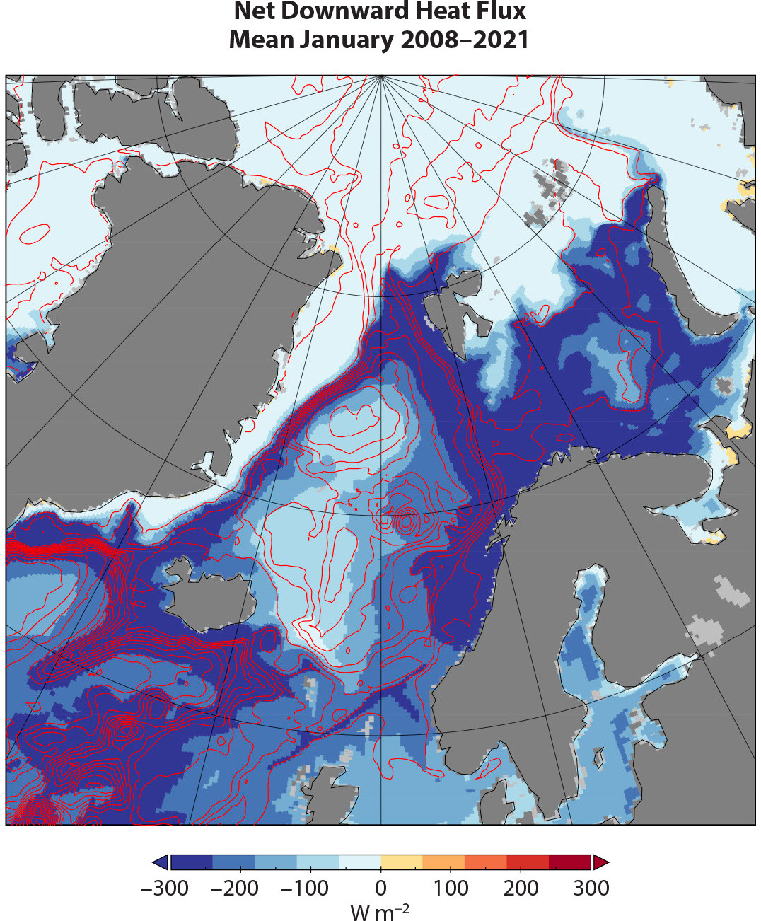
FIGURE 3. Net downward heat flux. Blues indicate ocean to atmosphere, and red contours show barotropic stream function (contour interval 4 Sv). January mean for 2008–2021 is from Nucleus for European Modelling of the Ocean (NEMO) 1/12º ice-ocean model with regional resolution of 3–5 km (Megann et al., 2021). Surface forcing is from JRA-55 (Tsujino et al., 2018, updated). > High res figure
|
The AMOC
Concerted measurement of the AMOC began in 2004 with the RAPID array1 of 19 moorings across the North Atlantic subpolar gyre, where the overturning circulation is readily defined in two parts—north-going warm and saline upper waters and south-going, colder, denser deep waters—and quantified on pressure surfaces (Frajka-Williams et al., 2019). However, this model is insufficient in the subpolar gyre because the AMOC possesses a third “leg” in the cold, fresh western boundary currents, and because the “flat” metric does not capture the water mass transformations that occur in the horizontal circulation. Instead, a “tilted” metric, based on density surfaces, is needed (Lozier et al. 2019). We can now clearly see the origin of this tripartite AMOC in the Arctic Ocean, with freshwater sourced in the subpolar boundary currents as well as in Nordic Seas heat loss and water mass modification. However, the apparent disappearance of the third leg between the subpolar and subtropical gyres presents a conundrum. Part of the answer is likely found in deep convection and deep winter mixing (in the Labrador, Irminger, and Iceland Seas) and in eddying, interior pathways (Bower et al., 2009) that inject waters into the deep, southward-flowing limb of the AMOC. But does vertical circulation at the front between the northern side of the North Atlantic Current and the interior of the gyre (e.g., Pollard and Regier, 1992), contribute to the change?
Long Surface Flux Time Series
The original expectation (or hope) driving the generation of Arctic net surface fluxes of heat and freshwater from ice and ocean measurements was based on their likely usefulness as independent resources in a data-sparse region, and we have shown that that expectation is being realized. Continuous measurement resources exist all around the Arctic Ocean boundary to extend the time series over two decades, from the early 2000s to the present, and it is to be hoped that this will happen sooner rather than later. As Mayer et al. (2019) point out, to resolve surface flux variability at sub-annual (monthly, seasonal) timescales requires knowledge of heat and freshwater storage and variability inside the boundary. Rabe et al. (2014) are beginning to be able to measure the interior seasonal cycle from in situ resources, and Armitage et al. (2016) show that wide-area remotely sensed measurements can detect mass and steric storage changes on monthly timescales. Perhaps a combination of the two can quantify the seasonal cycle.
Acknowledgments
We cannot acknowledge here the very many scientists, engineers, and marine staff from many countries who contributed to the many projects that generated the measurements employed in the research reviewed above, but we note that key analytical elements in the last 15 years were funded by the UK Natural Environment Research Council (NERC), projects ASBO and TEA-COSI, grants NE/D005965/1 and NE/I028947/1, and by the Norwegian Trond Mohn Foundation, grant BFS2016REK01. This paper is a contribution to UK NERC project CANARI (NE/W004984/1) and to project EPOC, EU grant 101059547 and UKRI grant 10038003.