Rapid assessment and enhanced knowledge of plankton communities and their structures in the productive upper water column is of crucial importance if we are to understand the impact of the changing climate on upper ocean processes. Enabling persistent and systematic ecosystem surveillance by coupling the revolution in robotics and automation with artificial intelligence (AI) methods will improve accuracy of predictions, reduce measurement uncertainty, and accelerate methodological sampling with high spatial and temporal resolution. Further, progress in real-time robotic visual sensing and machine learning have enabled high-​resolution space-time imaging, analysis, and interpretation. We describe a novel mobile robotic tool that characterizes upper water column biota by employing intelligent onboard sampling to target specific mesoplankton taxa. Although we focus on machine learning techniques, we also outline the processing pipeline that combines imaging, supervised machine learning, hydrodynamics, and AI planning. The tool we describe will accelerate the time-​consuming task of analyzing “who is there” and thus advance oceanographic observation.

A light autonomous underwater vehicle is shown following phytoplankton hotspots in the coastal waters near Munkholmen in Trondheimsfjorden. In the AILARON project, the vehicle uses a CTD, an onboard camera, and an acoustic Doppler current profiler along with adequate computing power. Photo credit: Annette Stahl/Norwegian University of Science and Technology, Trondheim, Norway. > High res figure

“With the ability to monitor planktonic patches at high spatiotemporal resolution on board a robotic vehicle, AILARON will provide a powerful and novel tool for biological oceanography, the equivalent of a robotic microplankton sniffer dog.”

 

Introduction

Studying planktonic standing stocks and community structure, including their spatial and temporal variability, provides significant insight into upper water column processes (Wasmund et al., 1998; Bojanić et al., 2005; Cornils et al., 2005; Bils et al., 2019). Collecting persistent and systematic observations of the upper water column is essential to biogeochemical research. Marine phytoplankton produce about 50% of the oxygen on our planet. Their biodiversity is critical to ecosystem stability, and they are responsible for primary productivity that supports higher trophic level consumers (Field et al., 1998; Malzahn et al., 2010; Boyce et al., 2015). Understanding the impact of global change and how key environmental variables (e.g., light, temperature, and salinity) affect plankton community structure is therefore critically important to our understanding of the future ocean (Johnsen et al., 2018; Fragoso et al., 2019). Previously, studies of plankton abundance and community structure have typically required expensive and time-consuming analyses of samples collected using ship-based or long-term monitoring approaches at discrete locations that often lack high spatiotemporal resolution.

Recent advances in artificial intelligence (AI), machine learning (ML), and robotics are now augmenting traditional methods of observation. Marine robots, especially autonomous underwater vehicles (AUVs; Rudnick and Perry, 2003; Bellingham and Rajan, 2007; Rudnick et al., 2018), have demonstrated the ability to provide continuous spatial and temporal observations, typically over the mesoscale. In addition, progress in computational science in the fields of real-time robotic visual sensing and ML have enabled inline high-resolution imaging, analysis, and interpretation. Bringing such computational methods to bear by augmenting current oceanographic approaches with agile and adaptive autonomous inferential capabilities that observe the environment at fine scales has become essential for understanding the changing ocean. In particular, a subset of machine learning, called deep learning (DL), utilizes neural networks (Qian, 1999), which we apply to microscopic robot visual sensor data. This nascent method shows substantial promise that we explore here.

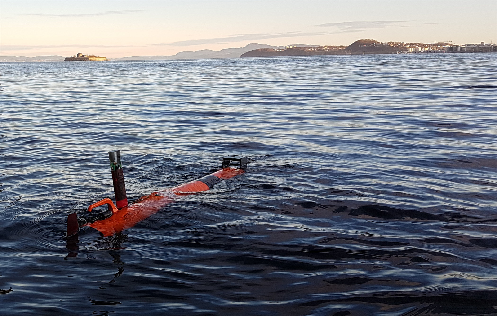
AILARON (Autonomous Imaging and Learning Ai RObot identifying plaNkton taxa in situ) is an interdisciplinary integrated effort that allows characterizing targeted plankton in situ. A camera aboard the AUV, shown in Figure 1, images planktontic organisms in the photic zone. This imagery is categorized and classified with onboard processing based on ML methods, and a probability density map is generated to show the spatial extent of various organisms imaged. In addition, an advanced AI-based controller is used to survey and facilitate return to the most coherent “hotspots” containing species of interest over the survey volume. The processing chain is guided by a human expert (as needed) via a communication link to shore. The operator can alter the vehicle’s sampling preferences dynamically, ensuring that the vehicle adapts on the fly. This process renders the AUV akin to a “sniffer dog” in that it maps out a volume for targeted ship-based, follow-on sampling, a task traditionally carried out by a scientist. Our approach contrasts with one taken by the Zooglider AUV (Ohman et al., 2019) in two critical ways. First, our AUV is powered and can adaptively target hotspots with onboard deliberation, while Zooglider follows a designated trajectory with adaptation directed by shore-side commands. Second, and the focus of this paper, we use ML onboard our vehicle to aid in situ adaptation for an end-to-end workflow.

 

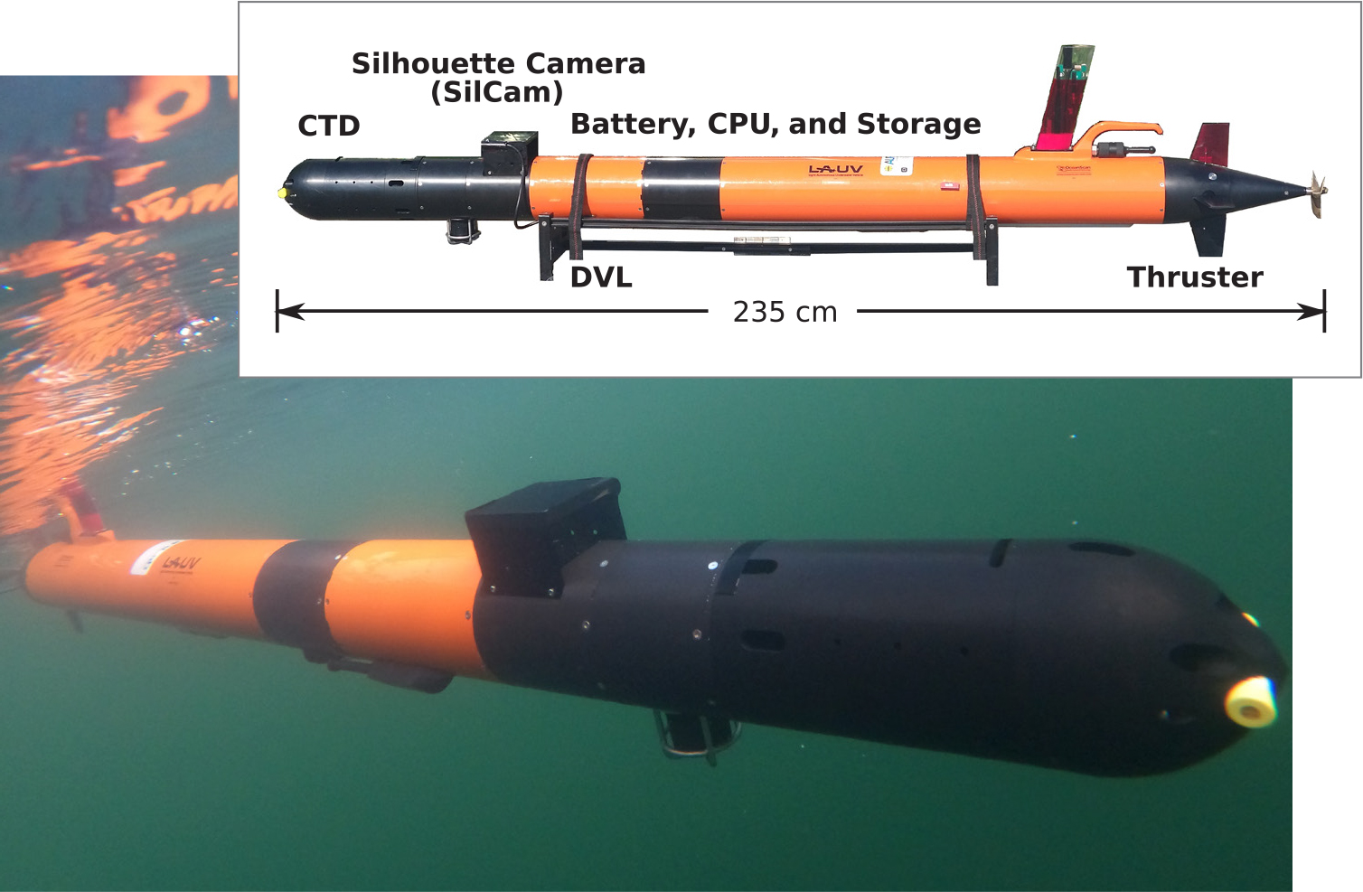
Figure 1. The human-portable light autonomous underwater vehicle (LAUV; Sousa et al., 2012) is shown navigating Trondheimsfjorden, Norway. Components include a silhouette camera (SilCam), a Doppler velocity log (DVL), and CTD sensors that are all used in AILARON (Autonomous Imaging and Learning Ai RObot identifying plaNkton taxa in situ). > High res figure

 

While we articulate the overall technical design and workflow of our system, our focus here is the novel integration of deep learning classifiers based on approaches for taxonomic estimates from time-series image analysis (Roberts and Jaffe, 2007; Sosik and Olson, 2008). The full imaging-classification-​analysis-​control workflow is embedded on an AUV. Integrating state-of-the-art methods from different engineering disciplines, embedding them onto a mobile robot, and deploying them as a proof of concept provides a new methodology for studying and understanding the variability of planktonic biomass and communities. Experimental results show promise that we expect will lead to significant future advancement of in situ plankton identification, assessment of biomass, and size fraction estimations.

 

Technical Approach

The key workflow component is the classifier, which follows DL approaches elaborated later in the section on Plankton Classification. The classifier aims to (1) filter detected objects, (2) categorize the organisms of interest, and (3) provide the number of detected species found per taxa. It is then integrated within an imaging-​classification-analysis-control workflow depicted in Figure 2, where boxes and lines in blue are online operations executed on board the AUV and those in orange are preprocessing tasks that are performed offline. The workflow is a continuous iterative process that starts with a camera capturing images from the water column in sequence and conveying them to the classifier for species detection and categorization. An in situ current model is generated from a Doppler velocity log. Volumetric information is obtained by combining this current model with tagged spatiotemporal data collected by the CTD and chlorophyll sensors on the AUV.¹ Using this information, the AI-based automated planning and execution engine (Rajan et al., 2013; Fossum et al., 2019) generates an estimated spatial map of different observed classes that, in turn, drives the AUV to systematically visit and sample the three-dimensional volume of locations of interest. Data collected by the onboard sensors in this volume help determine the spatial spread and volume of the targeted taxa before the AUV visits the next hotspot.

¹ Chlorophyll a indicates biomass of photosynthetic phytoplankton.

 

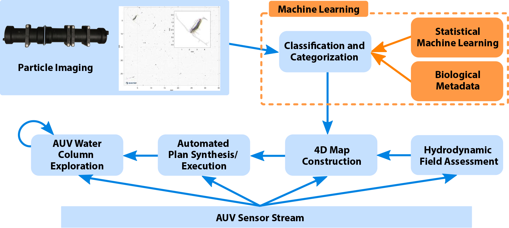
Figure 2. System workflow and operation for AILARON. Orange arrows and boxes indicate offline operations used as preprocessing steps to generate the classifier for underwater operations. Blue arrows and boxes represent continuously running operations on board the AUV and include imaging, classification, sensor evaluation, estimation, and plan execution. This paper focuses on methods that facilitate the modules within the dashed orange box. > High res figure

 

Plankton Classification

Our planktonic classifier is based on a DL algorithm, a concept inspired by the human biological neuron (McCulloch and Pitts, 1943). Deep learning methods are closely related to computational statistics (Gentle et al., 2012) and evolutionary approaches from the machine learning paradigm that aim to iteratively build a mathematical model from sample data. The resulting algorithm (or model), which applies optimization techniques, evolves by experience without explicit programming. The term “deep” connotes the number of layers and a combination of neurons (nodes) that are used to form the algorithmic architecture (Le et al., 2011). The DL algorithms are, in part, enabled due to the advent of computational power with multicore central processing units and general-purpose graphics processing units (GPUs). DL algorithms are state of the art in ML, especially for image-based object detection and classification, and they have been shown to outperform traditional classification approaches (Krizhevsky et al., 2012).

Given a large data set of input and output pairs, a DL algorithm will try to minimize the difference between its prediction and expected output. By doing so, it learns the association/pattern between given input and output data—that, in turn, allows such a model to generalize input data that it has not seen before (Choi et al., 2020). DL algorithms use neural networks to find associations between sets of input and output data. A DL algorithm comprises an input layer, hidden layers, and an output layer, all of which are composed of nodes. The input layer takes in a numerical representation of data (e.g., plankton image pixels), output layers output predictions (e.g., the plankton group affiliation), while hidden layers perform actual computation such as feature extraction from objects provided by the input layer. The setup and the number of layers utilized define the learning process and are specific to the problem being solved.

Hidden layers are mostly composed of convolutional layers. They extract features from objects based on a given image by applying convolution filtering, which processes spatial frequency features of an image to reveal object characteristics such as contours, edges, or curvatures. Most of the convolutional layers are followed by batch-normalization layers, which re­sample and scale the output of the convolutional layer to ensure stability and to improve the performance of the network, and max-pooling layers, which reduce the high-dimensional representation² of extracted features into fewer dimensions by replacing image intensity values with the maximal intensity value represented in that particular window. By doing so, each max-​pooling layer simplifies the complexity of the object/filter representation by combining correlated features, compressing them into those that are most important. This operation is highly nonlinear and leads to dimensionality reduction of the data, enabling an increase in computational efficiency during the learning process. The last sequence of fully connected layers groups lists of features and assigns them to classes.

² The resolution of an image or filter, for example, is given by 64 × 64 pixels.

There is a broad spectrum of ML methods, from supervised, to semi-supervised, to unsupervised learning, depending on prior knowledge and the input data set alongside the expected output. Supervised methods seek to learn higher-level representations from labeled data. A human domain expert assesses the data in a given context and tags it manually to its given taxa in order to develop a labeled data set. The DL algorithm, in turn, learns how to combine the higher-level representation of the data and matches this combination by assigning it to a certain class that is predefined by the domain expert. DL methods using supervised learning approaches achieve high accuracy that outperforms human recognition (Krizhevsky et al., 2012; Simonyan and Zisserman, 2015; Szegedy et al., 2015; Dai et al., 2016; He et al., 2016; Lee et al., 2016; Py et al., 2016; Moniruzzaman et al., 2017). Unsupervised algorithms, on the other hand, without manual labeling, help discover hidden patterns in the data by, for example, clustering operations, and perform dimensionality reduction by projecting high-dimensional data down to fewer dimension clusters or classes (Min et al., 2009; Xie et al., 2016; Kuzminykh et al., 2018).

Because our AUV moves through the water column taking images continuously, we explored multiple approaches for time-series image analysis and in situ classification (Roberts and Jaffe, 2007; Sosik and Olson, 2008) and investigated the applicability of supervised DL mechanisms in order to find the best performing method.

The chosen Deep Learning Neural Network implementation, shown in Figure 3, reported an accuracy of 95% as opposed to 90%–93% achieved by state-of-the-art neural networks such as ZooplanktoNet (Dai et al., 2016), VGGNet (Simonyan and Zisserman, 2015), AlexNet (Krizhevsky et al., 2012), ResNet (He et al., 2016), and GoogleNet (Szegedy et al., 2015), while training over a labeled data set of extracted objects from images of plankton organisms captured in situ and manually labeled by biologists (Table 1). The selected DL implementation, depicted in Figure 3, with five convolutional layers, shows good performance for real-time in situ classification.

 

 

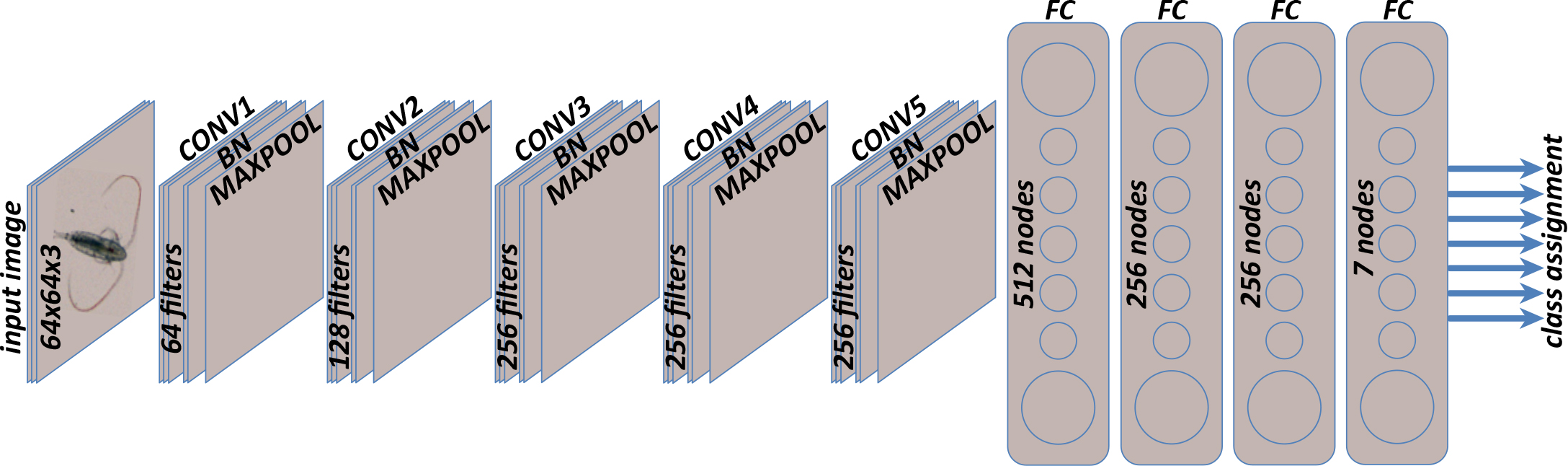
Figure 3. The deep learning neural network implementation transforms an input image (high-dimensional representation) into a class assignment (lower-dimensional representation) via five convolutional layers (CONV) for feature extraction, interleaved with batch-normalization layers (BN) for resampling and max-pooling layers (MAXPOOL) for dimensionality reduction, followed by four fully connected layers (FC) for feature to class assignment. The input image format is RGB of size 64 × 64 × 3 (width × height × number of channels) in pixels. Each RGB color is saved in a separate channel. > High res figure

 

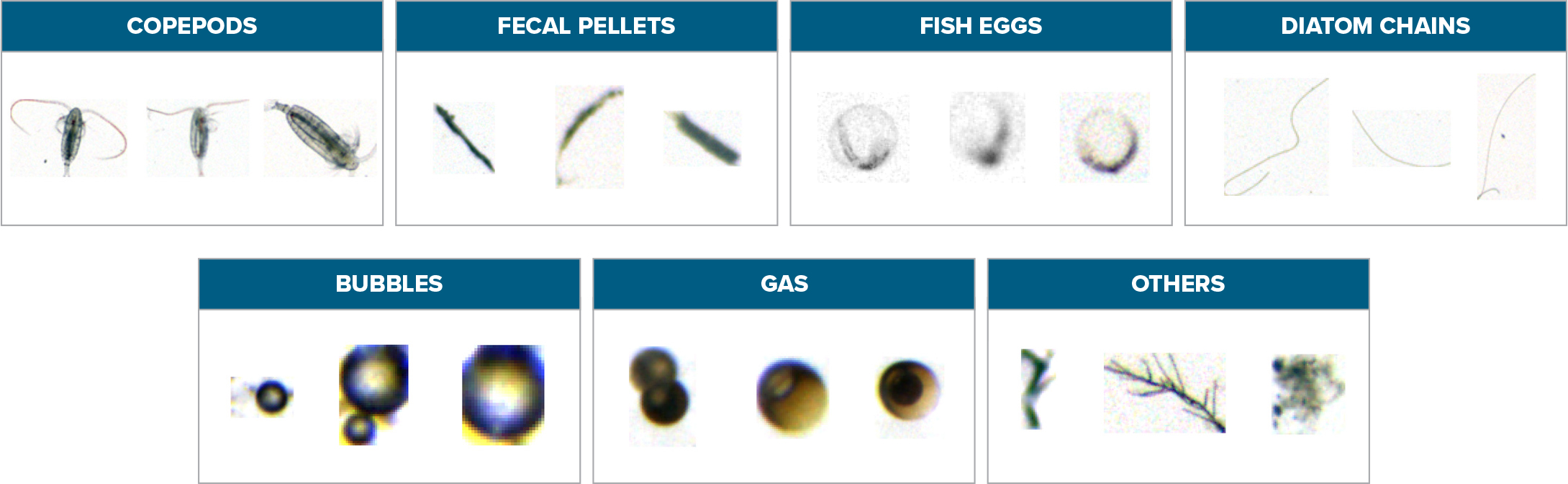
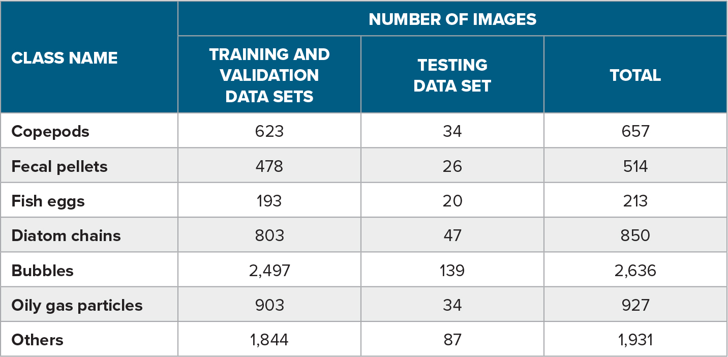
The training process for a supervised learning algorithm iteratively builds up the mathematical model from a labeled data set through the sequence of combined neural layers. It does so by applying a gradient descent algorithm (Qian, 1999) that measures the effect of changing the input on the produced output. This effect is controlled by updating the weights of the nodes forming the layers while minimizing a predefined loss function, namely cross-entropy (De Boer et al., 2005). The latter indicates how the output of the classification is diverging from the ground truth labels. This technique, known as backpropagation (Scalero and Tepedelenlioglu, 1992; Chauvin and Rumelhart, 1995), runs over a labeled data set provided to the algorithm as prior knowledge. Table 1 contains example images from a database (Davies et al., 2018) with a set of 7,728 individual planktonic images representing seven different classes that have been tagged and classified manually by biologists. Table 2 lists the class distribution of the planktonic taxa representation in the labeled database, with the training and validation sets forming 95% of the full database and the test set 5%. The state-of-the-art approaches for training the model over an imbalanced data set were adopted by Dai et al., 2016. The algorithm utilizes batches from the training images in order to learn to map objects to the final set of classes. The validation set verifies the success of the algorithm to optimize the loss function after each batch run and accordingly updates the weights of the internal nodes. The train-validate loop runs until convergence or a stage where the difference in the output loss is negligible. The test set is kept to evaluate the algorithm’s accuracy and performance after the training process. Both training and testing processes are performed offline through the deep learning algorithm (orange boxes in Figure 4), on two GPUs of ASUS RTX2080Ti Turbo with a 64 GB RAM, where the training is performed over 200 epochs, with each epoch taking an average of 81 seconds.

 

Table 1. Instances of a labeled data set (Davies et al., 2018) of objects extracted from in situ images and labeled manually by biologists as a prerequisite for the training process. > High res figure

 

Table 2. The class distribution representation in the labeled data set used in the training process. > High res figure

 

To test the performance of the trained algorithm, the set of images from the test set, unknown to the model, are fed into the system to predict corresponding classes. The terms true-positive, true-​negative, false-positive, and false-​negative represent the correct and falsely allocated images with respect to specific classes. They are utilized to define model accuracy; in our case, the DL implementation depicted in Figure 3 reported an accuracy of 95% when tested on a set of ~1,000 images that the algorithm had not seen before.

 

The Online Prediction Module

The online prediction module (Figure 4) implements three essential steps executed aboard the AUV: (1) segmentation, which aims to extract objects when they appear in the captured frame from time-series images; (2) identification and classification, based on the DL classifier, which learns a function that maps high dimensional representations of the input images to low dimensional output data (prediction of the class assignment); and (3) calculation of the class distribution, which deduces, from time-​series information of images, the number of detected objects per taxa to provide their distribution with respect to location and time. The three steps are performed aboard the AUV on an NVIDIA Jetson TX2 SSD 500GB mSATA with 2 TB storage. As shown by the blue boxes in Figure 4, the onboard silhouette camera (SilCam; Davies et al., 2017) captures images in sequence at a rate of five frames per second. Once captured, each image is queued in a buffer for processing, which is done in parallel. Each image is processed in 3.852 seconds on average. The processing time depends on the number of objects extracted from the image. The average time taken per step in the sequence is 0.622 seconds for background correction, 0.458 seconds for segmentation, and 0.02 seconds to predict the class of each extracted object from the image. The measurement of class distribution outputs a mix of known and unknown taxa, which is then manually verified and tagged by the biologist through an offline process to update the knowledge base.

 

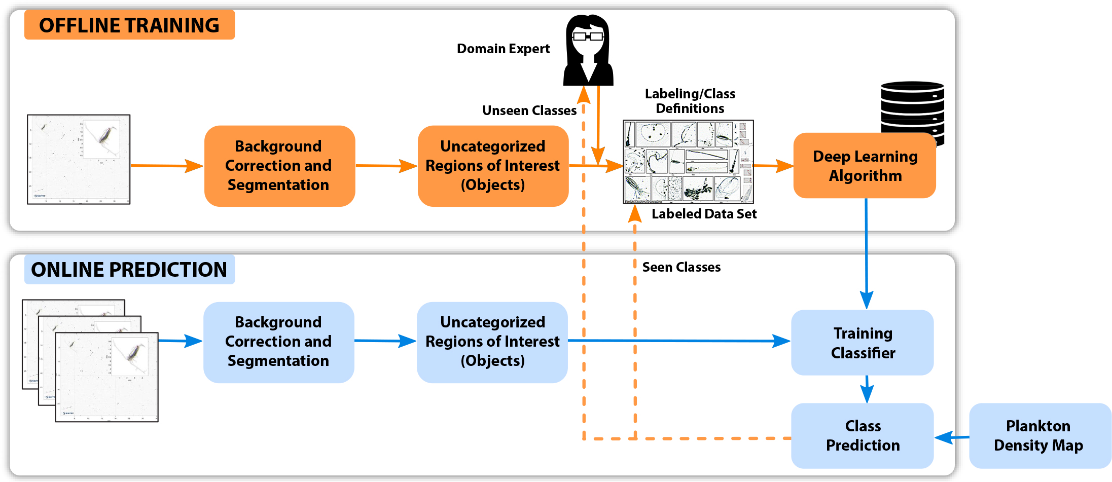
Figure 4. Block diagram of the classifier, from object identification, classification, and categorization to producing a plankton density map on the AUV. Supervised machine learning occurs offline to build a model, which is consulted during online classification. The dotted arrows from “class prediction” represent the predicted objects in situ. Each object belongs to one of the following two types: seen classes (the algorithm was trained on this category) and unseen classes (the algorithm was never trained on these classes, hence, the domain expert is consulted to update the data set). The figure shows offline tasks in orange arrows and boxes and onboard in situ processing in blue. > High res figure

 

Step 1: Object Identification and Localization

https://github.com/SINTEF/PySilCam

A background correction algorithm subtracts a sliding average window of a set of images from each analyzed image to remove noise and to detect changes occurring in the time series. The background-​corrected image is then converted into binary form to extract the foreground objects following a thresholding technique that uses a fast segmentation approach (Zhu et al., 2007; van der Walt et al., 2014). Each connected region forms an extracted object. Connected regions are then counted and localized to infer the number of extracted objects and their places in the image as well as in the time series.

Step 2: Extracted Object Classification

https://github.com/AILARON/silcam_​supervised_classification

The number of extracted objects from the previous step is an aggregated representation of all existing foreground particles irrespective of the class to which each object belongs. Each object, forming a connected region, is then passed to the classifier. The trained model, in turn, filters the objects of interest and associates to each a probability measure indicating the likelihood the object belongs to a specific taxa.

Step 3: Measurement of Class Distribution

https://github.com/AILARON/silcam_​supervised_classification

The inferred probabilities are logged along with spatial and temporal information for each detected particle in the image.

Figure 4 shows the iterative nature of this classification process. Extracted objects that do not belong to any of the predefined classes and fall into the “others” category are validated manually by domain experts, who update the knowledge base offline. This evolving database is then used to train the model for future detection of all species identified.

 

System Integration and Experimental Results

The full system of imaging-classification-​analysis-​control workflow, briefly described in the section above on Technical Approach, contains the DL classifier and is integrated on board an AUV.

A SilCam captures images of an equivalent circular diameter >108 mm, where the captured volume is 75.6 cm³ (45 mm × 56 mm × 30 mm). The pixel resolution of the produced images is 27.5 μm. Captured images belong to classes of planktonic organisms such as copepods (Calanoida) and diatom chains (Thalassiosira spp., Chaetoceros spp., and Skeletonema spp.). Time-series images, captured at five frames per second, are then fed into the DL-based image classification system. The classifier assigns a probability to each detected object, showing how likely it is that an object belongs to a given class. When the assigned probability is >95%, the object is then counted in the respective class and the class concentration of organisms is updated. The histograms of organism concentration in Figure 5 show identified copepods and diatom chains at >95% likelihood taken at four-meter intervals. The concentration is the number of species (per liter) detected by the AUV in the water column. The number of diatoms is regulated by key environmental variables and zooplankton (e.g., copepods) grazing pressure and is affected by prey and predator size and species. Figure 6 shows that there were slightly lower copepod densities at 10–20 m depth, while higher numbers were found at depths between 20 m and 25 m. At depths greater than 28 m, no copepods were found. These findings exemplify a post-​spring-​bloom situation (in this case, April 23) in Trondheimsfjorden, Norway. Post-​blooms of phytoplankton in this area are generally characterized by a decline in the number of diatoms (Volent et al., 2011).

 

Figure 5. Histogram of organism concentration for identified copepods and diatom chains at >95% likelihood, in Trondheimsfjorden, Norway, taken at four-​meter intervals in April 2020. > High res figure

 

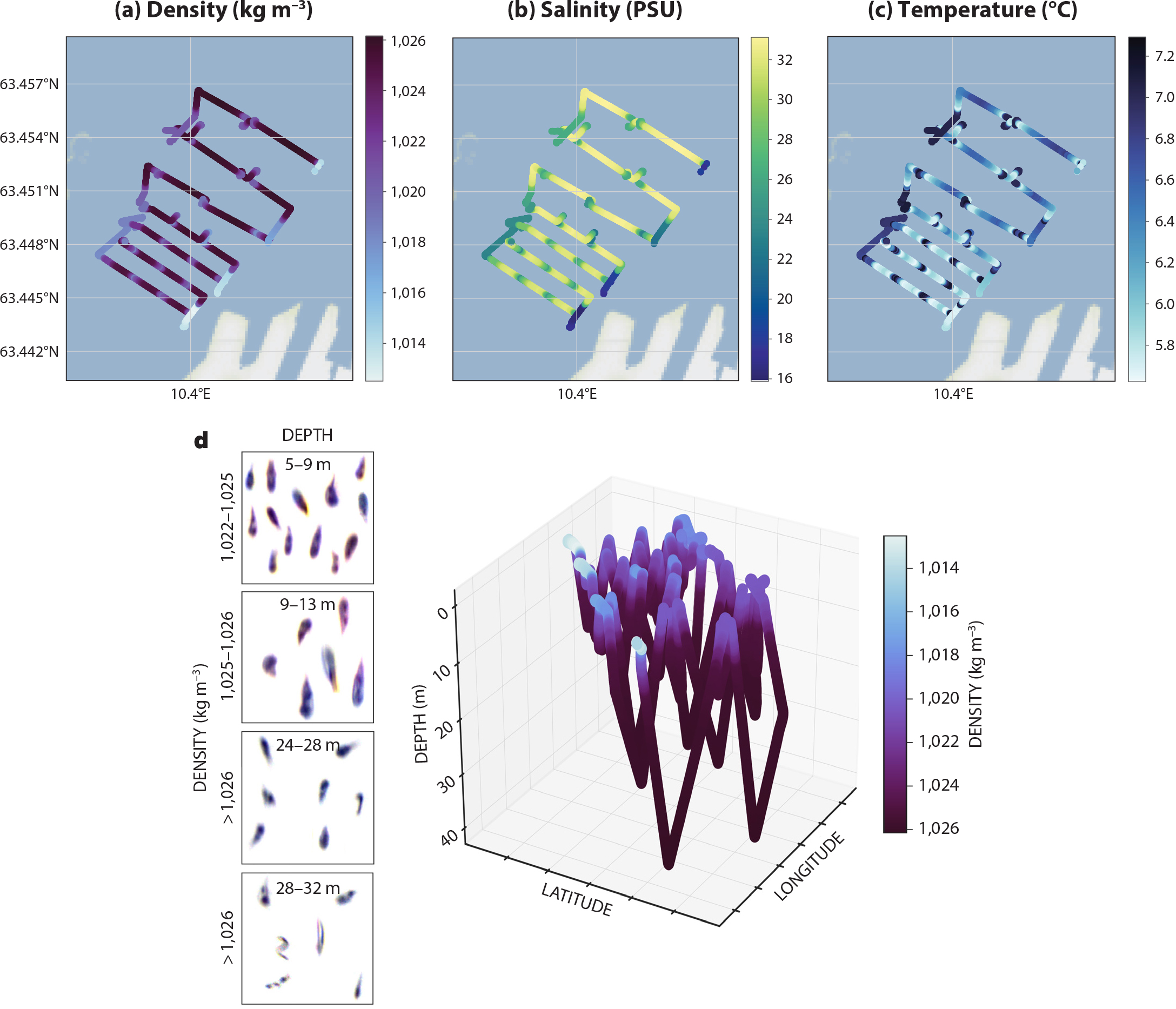
Figure 6. (a) Density (kg m–3), (b) salinity (PSU), (c) temperature (°C), and (d) three-​dimensional density (kg m–3) snapshots of detected planktontic organisms, in this case mainly copepods, the dominant taxa with respect to biomass in distinct water layers. Data are from an April 2020 AUV mission in Trondheimsfjorden, Norway. > High res figure

 

Organism concentration per group is then conveyed to the next step in the workflow to highlight community structure and spatial distribution in the water column. The output is a concentration estimate for each group, with corresponding uncertainty estimates provided by the probability distribution, median, mean, and standard deviation. These uncertainty estimates, in turn, are used to continuously update a probability density map that shows community dispersion in three dimensions. This information is now used to generate a map of hotspots that directs an adaptive sampling process with the automated planning and execution engine.

Below, we briefly discuss the functionalities related to dynamic flow estimation and automated plan execution because of their importance to the overall context for machine learning; however, their details are outside the scope of this article.

Hydrodynamics

To predict future positions of any observed plankton hotspots as they are advected with currents requires a model of the local hydrodynamics. For these computations, the flow must be evaluated at arbitrary locations inside and outside of the volume covered by the initial survey. From an initial survey, a set of velocity profiles are obtained using a Doppler velocity log on the AUV. After discarding measurements of poor quality, interpolation and extrapolation are used to create a local estimate of the currents at different depth layers.

Once an estimate of the local hydrodynamics has been obtained from the initial survey, a Lagrangian particle transport model (van Sebille et al., 2018) is applied to predict the temporal evolution of plankton concentration in space. Numerical particles representing different types of plankton are seeded over the volume of the initial survey, with measured plankton concentrations. Each particle is transported individually through the current field using a fixed or variable-time step integrator (Nordam and Duran, 2020), applying a random walk to reflect the uncertainty in the measured currents, and optionally adding any active “swimming” behavior according to time of day and plankton type.

Automated Planning and Execution

The overall operational concept is for our AUV to adaptively visit planktonic hotspots as they advect in the water column after an initial fixed “lawn mower” survey. Such adaptivity requires deliberative decision-making using sensor input while projecting the future state in order to achieve stated goals or outcomes (Ghallab et al., 2016). Plan generation and execution embedded on a robot is continuous, dynamically adapting to the continuous sensory input from the robot’s environment. This input updates the internal plan representation that in turn can alter future actions by replanning or plan synthesis. In enabling this continuous sense-plan-act loop, the robot can adapt to changing conditions in the real world, enabling a level of cognitive capacity not available on most robotic vehicles to date. We employ a mature onboard planning​/​execution software engine (Rajan et al., 2013; Fossum et al., 2019) that uses the input from classification to estimate a spatial probability density of the plankton-taxa classes as a spatiotemporal Gaussian process (GP; MacKay, 1998). The hydrodynamic model is used to project a hotspot location that, when visited by the vehicle, uses a GP to systematically map an individual density field. The estimated GP and the planned path are continuously updated as new measurements are gathered along a trajectory.

 

Discussion

The use of machine learning methods in flow cytometry (Kalmbach et al., 2017) has provided new insights into planktonic communities. However, to understand how community structure and dispersion correlate with water-column biological processes, they must be studied in situ and mapped at scale. Powered AUVs have proven to be robust and adaptive with sufficient capability for onboard computation, in addition to long in-water residence time (our vehicle, for example, can operate for upwards of 48 hours). AUVs have the necessary computing power to operate the pipeline proposed in this project. Furthermore, they have the computational and propulsive capacity to be able to “return” to a hotspot, making the sampling more adaptive. Integrative capacity to image, categorize, model, and command on board such a low-cost vehicle can ensure rapid spread of such a find-tag-follow capability for planktonic biomass.

However, some technological challenges remain. Foremost among them is the ability to obtain and manually label a large image data set at similar magnification for classification accuracy. Saad et al. (2020) proved that ML approaches for object instance and semantic segmentation perform better on the SilCam captured images in terms of speed and accuracy. Embedding such approaches into the framework and deploying them online can help to speed up the system processing of the images captured in sequence. Additionally, these approaches might allow the number of captured frames per second to be increased. Second, to date we have only a limited number of classes available for detection (Table 1), in large part because of the scale of labeling and data collection needed. The data collected belong to the Trondheimsfjorden environment to ensure that the concept is viable in our local domain. As we increase the number of AUV missions, we expect to provide a diverse set of classes while enabling the framework to work across different environments. Third, advances in imaging resolution that would allow higher taxonomic classification and imaging for microplankton <200 μm is still in infancy. Last but not the least, motility of zooplankton with distinct avoidance behavior, likely due to the disturbance of the flow around the vehicle when it is moving rapidly, requires fine calibration of vehicle dynamics or substantial variation of trajectory planning, a challenge with any form of mobility in the water column.

 

Conclusion

Abundance and organism identification require careful and repetitive work, which can now be enhanced by new techniques in robotic vision, classification, and categorization using deep learning methods, as we have described. The novelty presented here lies in embedding these advances in an autonomous robot that can then be tasked using mature methods in sampling, sensor fusion, hydrodynamics, and autonomous systems to revisit microorganism hotspots. AILARON is the first to apply the entire chain of imaging-​classification-​analysis-​control to plankton taxa classification, in particular, on board a mobile robotic platform. With the ability to monitor planktonic patches at high spatiotemporal resolution on board a robotic vehicle, AILARON will provide a powerful and novel tool for biological oceanography, the equivalent of a robotic microplankton sniffer dog. In doing so, it will provide enhanced knowledge of plankton communities and their spatiotemporal distribution patterns, which have great importance for ecosystem surveillance and monitoring global change effects.

 

Acknowledgments

This work was supported by the Research Council of Norway (RCN) IKTPLUSS program, project #262741 and AMOS RCN #223254. The authors are grateful to Bjarne Kvæstad for discussions on deep learning and to Joe Garrett for his constructive feedback on an early version of this manuscript.

Saad, A., A. Stahl, A. Våge, E. Davies, T. Nordam, N. Aberle, M. Ludvigsen, G. Johnsen, J. Sousa, and K. Rajan. 2020. Advancing ocean observation with an AI-driven mobile robotic explorer. Oceanography 33(3):50–59, https://doi.org/10.5670/oceanog.2020.307.

Bellingham, J.G., and K. Rajan. 2007. Robotics in remote and hostile environments. Science 318(5853):1,098–1,102, https://doi.org/​10.1126/science.1146230.
1. Bils, F., M. Moyano, N. Aberle, C.J.G. Van Damme, R.D.M. Nash, M. Kloppmann, C. Loots, and M.A. Peck. 2019. Broad-scale distribution of the winter protozooplankton community in the North Sea. Journal of Sea Research 144:112–121, https://doi.org/10.1016/j.seares.2018.11.006.
2. Bojanić, N., M. Šolić, N. Krstulović, S. Šestanović, I. Marasović, and Ž. Ninčević. 2005. Temporal variability in abundance and biomass of ciliates and copepods in the eutrophicated part of Kaštela Bay (Middle Adriatic Sea). Helgoland Marine Research 59(2):107–120, https://doi.org/10.1007/s10152-004-0199-x.
3. Boyce, D.G., K.T. Frank, B. Worm, and W.C. Leggett. 2015. Spatial patterns and predictors of trophic control in marine ecosystems. Ecology Letters 18(10):1,001–1,011, https://doi.org/10.1111/ele.12481.
4. Chauvin, Y., and D.E. Rumelhart. 1995. Backpropagation: Theory, Architectures, and Applications. Psychology Press, 576 pp.
5. Choi, R.Y., A.S. Coyner, J. Kalpathy-Cramer, M.F. Chiang, and J.P. Campbell. 2020. Introduction to machine learning, neural networks, and deep learning. Translational Vision Science & Technology 9(2):14–14.
6. Cornils, A., S.B. Schnack-Schiel, W. Hagen, M. Dowidar, N. Stambler, O. Plähn, and C. Richter. 2005. Spatial and temporal distribution of mesozooplankton in the Gulf of Aqaba and the northern Red Sea in February/March 1999. Journal of Plankton Research 27(6):505–518, https://doi.org/​10.1093/plankt/fbi023.
7. Dai, J., R. Wang, H. Zheng, G. Ji, and X. Qiao. 2016. ZooplanktoNet: Deep convolutional network for zooplankton classification. Pp. 1–6 in Proceedings of OCEANS 2016-Shanghai. IEEE, https://doi.org/​10.1109/OCEANSAP.2016.7485680.
8. Davies, E.J., P.J. Brandvik, F. Leirvik, and R. Nepstad. 2017. The use of wide-band transmittance imaging to size and classify suspended particulate matter in seawater. Marine Pollution Bulletin 115(1–2):105–114, https://doi.org/10.1016/j.marpolbul.2016.11.063.
9. Davies, E.J., A. Ahnell, F. Leirvik, and P.J. Brandvik. 2018. Optical monitoring of subsea blowout droplets and subsea dispersant efficacy. Paper presented at the Forty-First AMOP Technical Seminar, Environment and Climate Change, Ottawa, ON, Canada.
10. De Boer, P.-T., D.P. Kroese, S. Mannor, and R.Y. Rubinstein. 2005. A tutorial on the cross-​entropy method. Annals of Operations Research 134(1):19–67, https://doi.org/10.1007/s10479-005-5724-z.
11. Field, C.B., M.J. Behrenfeld, J.T. Randerson, and P. Falkowski. 1998. Primary production of the biosphere: Integrating terrestrial and oceanic components. Science 281(5374):237–240, https://doi.org/​10.1126/science.281.5374.237.
12. Fossum, T.O., G.M. Fragoso, E.J. Davies, J.E. Ullgren, R. Mendes, G. Johnsen, I. Ellingsen, J. Eidsvik, M. Ludvigsen, and K. Rajan. 2019. Toward adaptive robotic sampling of phytoplankton in the coastal ocean. Science Robotics 4(27):eaav3041, https://doi.org/10.1126/scirobotics.aav3041.
13. Fragoso, G.M., E.J. Davies, I. Ellingsen, M.S. Chauton, T. Fossum, M. Ludvigsen, K.B. Steinhovden, K. Rajan, and G. Johnsen. 2019. Physical controls on phytoplankton size structure, photophysiology and suspended particles in a Norwegian biological hotspot. Progress in Oceanography 175:284–299, https://doi.org/10.1016/j.pocean.2019.05.001.
14. Gentle, J.E., W.K. Härdle, and Y. Mori, eds. 2012. Handbook of Computational Statistics: Concepts and Methods, 2^nd ed. Springer Science & Business Media, 1,204 pp.
15. Ghallab, M., D. Nau, and P. Traverso. 2016. Automated Planning and Acting. Cambridge University Press, 368 pp.
16. He, K., X. Zhang, S. Ren, and J. Sun. 2016. Deep residual learning for image recognition. Pp. 770–778 in Proceedings of 2016 IEEE Conference on Computer Vision and Pattern Recognition. https://doi.org/​10.1109/CVPR.2016.90.
17. Johnsen, G., M. Norli, M. Moline, I. Robbins, C. von Quillfeldt, K. Sørensen, F. Cottier, and J. Berge. 2018. The advective origin of an under-ice spring bloom in the Arctic Ocean using multiple observational platforms. Polar Biology 41(6):1,197–1,216, https://doi.org/10.1007/s00300-018-2278-5.
18. Kalmbach, A., Y. Girdhar, H.M. Sosik, and G. Dudek. 2017. Phytoplankton hotspot prediction with an unsupervised spatial community model. Pp. 4,906–4,913 in Proceedings of the 2017 IEEE International Conference on Robotics and Automation (ICRA). https://doi.org/10.1109/ICRA.2017.7989568.
19. Krizhevsky, A., I. Sutskever, and G.E. Hinton. 2012. ImageNet classification with deep convolutional neural networks. Paper presented at Advances in Neural Information Processing Systems 25: 26th Annual Conference on Neural Information Processing Systems, December 3–6, 2012, Lake Tahoe, NV.
20. Kuzminykh, D., D. Polykovskiy, and A. Zhebrak. 2018. Extracting invariant features from images using an equivariant autoencoder. Paper presented at the Asian Conference on Machine Learning, 2018, November 14–16, 2018, Beijing, China.
21. Le, Q.V., J. Ngiam, A. Coates, A. Lahiri, B. Prochnow, and A.Y. Ng. 2011. On optimization methods for deep learning. Pp. 265–272 in Proceedings of the International Conference on Machine Learning.
22. Lee, H., M. Park, and J. Kim. 2016. Plankton classification on imbalanced large scale database via convolutional neural networks with transfer learning. Pp. 3,713–3,717 in Proceedings of the 2016 IEEE International Conference on Image Processing (ICIP). IEEE, https://doi.org/10.1109/ICIP.2016.7533053.
23. MacKay, D.J.C. 1998. Introduction to Gaussian processes. NATO ASI Series F Computer and Systems Sciences 168:133–166.
24. Malzahn, A.M., F. Hantzsche, K.L. Schoo, M. Boersma, and N. Aberle. 2010. Differential effects of nutrient-​limited primary production on primary, secondary or tertiary consumers. Oecologia 162(1):35–48, https://doi.org/10.1007/s00442-009-1458-y.
25. McCulloch, W.S., and W. Pitts. 1943. A logical calculus of the ideas immanent in nervous activity. The Bulletin of Mathematical Biophysics 5(4):115–133, https://doi.org/10.1007/BF02478259.
26. Min, M.R., D.A. Stanley, Z. Yuan, A. Bonner, and Z. Zhang. 2009. Large-margin KNN classification using a deep encoder network. Paper presented at the Ninth IEEE International Conference on Data Mining, ICDM.
27. Moniruzzaman, M., S.M.S. Islam, M. Bennamoun, and P. Lavery. 2017. Deep learning on underwater marine object detection: A survey. Pp. 150–160 in Proceedings of the International Conference on Advanced Concepts for Intelligent Vision Systems. Springer, https://doi.org/​10.1007/​978-3-319-70353-4_13.
28. Nordam, T., and R. Duran. 2020. Numerical integrators for Lagrangian oceanography. Geoscientific Model Development Discussions, https://doi.org/​10.5194/gmd-2020-154.
29. Ohman, M.D., R.E. Davis, J.T. Sherman, K.R. Grindley, B.M. Whitmore, C.F. Nickels, and J.S. Ellen. 2019. Zooglider: An autonomous vehicle for optical and acoustic sensing of zooplankton. Limnology and Oceanography: Methods 17(1):69–86, https://doi.org/​10.1002/lom3.10301.
30. Py, O., H. Hong, and S. Zhongzhi. 2016. Plankton classification with deep convolutional neural networks. Pp. 132–136 in Proceedings of the 2016 Information Technology, Networking, Electronic and Automation Control Conference. IEEE, https://doi.org/10.1109/ITNEC.2016.7560334.
31. Qian, N. 1999. On the momentum term in gradient descent learning algorithms. Neural Networks 12(1):145–151, https://doi.org/10.1016/S0893-6080(98)00116-6.
32. Rajan, K., F. Py, and J. Barreiro. 2013. Towards deliberative control in marine robotics. Pp. 91–175 in Marine Robot Autonomy. M.L. Seto, ed., Springer, https://doi.org/10.1007/978-1-4614-5659-9_3.
33. Roberts, P.L.D., and J.S. Jaffe. 2007. Multiple angle acoustic classification of zooplankton. The Journal of the Acoustical Society of America 121(4):2,060–2,070, https://doi.org/​10.1121/1.2697471.
34. Rudnick, D.L., and M.J. Perry. 2003. ALPS: Autonomous and Lagrangian Platforms and Sensors. A report of the workshop held March 31–April 2, 2003, La Jolla, CA, 64 pp.
35. Rudnick, D., D. Costa, K. Johnson, C. Lee, and M.L. Timmermans. 2018. ALPS II-Autonomous and Lagrangian Platforms and Sensors. A Report of the ALPS II Workshop, held February 21–24, 2017, La Jolla, CA, 66 pp.
36. Saad, A., S. Bergum, and A. Stahl. 2020. An instance segmentation framework for in-situ plankton taxa assessment. Paper presented at ICMV 202: The Thirteenth International Conference on Machine Vision, Rome, Italy, November 2–6, 2020.
37. Scalero, R.S., and N. Tepedelenlioglu. 1992. A fast new algorithm for training feedforward neural networks. IEEE Transactions on Signal Processing 40(1):202–210, https://doi.org/​10.1109/​78.157194.
38. Simonyan, K., and A. Zisserman. 2015. Very deep convolutional networks for large-scale image recognition. Paper presented at the International Conference on Learning Representations, San Diego, CA, May 7–9, 2015.
39. Sosik, H.M., and R.J. Olson. 2008. New technologies to acquire time series of phytoplankton community structure: Submersible image-in-flow cytometry and automated taxonomic classification. Proceedings of Ocean Optics XVIII, 15 pp.
40. Sousa, A., L. Madureira, J. Coelho, J. Pinto, J. Pereira, J.B. Sousa, and P. Dias. 2012. LAUV: The man-portable autonomous underwater vehicle. International Federation of Automatic Control Proceedings 45(5):268–274, https://doi.org/​10.3182/20120410-3-PT-4028.00045.
41. Szegedy, C., W. Liu, Y. Jia, P. Sermanet, S. Reed, D. Anguelov, D. Erhan, V. Vanhoucke, and A. Rabinovich. 2015. Going deeper with convolutions. Pp. 1–9 in Proceedings of the 2015 IEEE Conference on Computer Vision and Pattern Recognition. https://doi.org/10.1109/CVPR.2015.7298594.
42. van der Walt, S., J.L. Schönberger, J. Nunez-Iglesias, F. Boulogne, J.D. Warner, N. Yager, E. Gouillart, T. Yu, and the scikit-image contributors. 2014. Scikit-image: Image processing in Python. PeerJ 2:e453, https://doi.org/10.7717/peerj.453.
43. van Sebille, E., S.M. Griffies, R. Abernathey, T.P. Adams, P. Berloff, A. Biastoch, B. Blanke, E.P. Chassignet, Y. Cheng, and C.J. Cotter. 2018. Lagrangian ocean analysis: Fundamentals and practices. Ocean Modelling 121:49–75, https://doi.org/10.1016/j.ocemod.2017.11.008.
44. Volent, Z., G. Johnsen, E.K. Hovland, A. Folkestad, L.M. Olsen, K. Tangen, and K. Sorensen. 2011. Improved monitoring of phytoplankton bloom dynamics in a Norwegian fjord by integrating satellite data, pigment analysis, and Ferrybox data with a coastal observation network. Journal of Applied Remote Sensing 5(1):1–22, https://doi.org/​10.1117/1.3658032.
45. Wasmund, N., G. Nausch, and W. Matthäus. 1998. Phytoplankton spring blooms in the southern Baltic Sea—Spatio-temporal development and long-term trends. Journal of Plankton Research 20(6):1,099–1,117, https://doi.org/10.1093/plankt/20.6.1099.
46. Xie, J., R. Girshick, and A. Farhadi. 2016. Unsupervised deep embedding for clustering analysis. Paper presented at the International Conference on Machine Learning, 10 pp.
47. Zhu, S., X. Xia, Q. Zhang, and K. Belloulata. 2007. An image segmentation algorithm in image processing based on threshold segmentation. Pp. 673–678 in Proceedings of the 2007 Third International IEEE Conference on Signal-Image Technologies and Internet-Based System. IEEE, https://doi.org/10.1109/SITIS.2007.116.

This is an open access article made available under the terms of the Creative Commons Attribution 4.0 International License (https://creativecommons.org/licenses/by/4.0/), which permits use, sharing, adaptation, distribution, and reproduction in any medium or format as long as users cite the materials appropriately, provide a link to the Creative Commons license, and indicate the changes that were made to the original content. Images, animations, videos, or other third-party material used in articles are included in the Creative Commons license unless indicated otherwise in a credit line to the material. If the material is not included in the article’s Creative Commons license, users will need to obtain permission directly from the license holder to reproduce the material.