The chemistry of the global ocean is rapidly changing due to the uptake of anthropogenic carbon dioxide (CO₂). This process, commonly referred to as ocean acidification (OA), is negatively impacting many marine species and ecosystems. In this study, we combine observations in the global surface ocean collected by NOAA Pacific Marine Environmental Laboratory and Atlantic Oceanographic and Meteorological Laboratory scientists and their national and international colleagues over the last several decades, along with model outputs, to provide a high-​resolution, regionally varying view of global surface ocean carbon dioxide fugacity, carbonate ion content, total hydrogen ion content, pH on total scale, and aragonite and calcite saturation states on selected time intervals from 1961 to 2020. We discuss the major roles played by air-sea anthropogenic CO₂ uptake, warming, local upwelling processes, and declining buffer capacity in controlling the spatial and temporal variability of these parameters. These changes are occurring rapidly in regions that would normally be considered OA refugia, thus threatening the protection that these regions provide for stocks of sensitive species and increasing the potential for expanding biological impacts.

Global surface ocean pH on total scale in 2020. Modified from Jiang et al. (2023). > High res figure

Introduction

Ocean chemistry is changing due to the uptake of anthropogenic CO₂ from the atmosphere (DeVries, 2022). Since the beginning of the industrial revolution in the eighteenth century, the global ocean has absorbed about 170 Gt C as carbon dioxide (1 Gt C is equivalent to 1 billion metric tons of carbon, or 3.667 billion metric tons of CO₂) via the combined impacts of human activities, including fossil fuel use for energy, land use changes, and cement production (Friedlingstein et al., 2020, 2022; Gruber et al., 2023). Upon exchanging with seawater at the air-sea interface, anthropogenic CO₂ combines with seawater to form carbonic acid, which increases the hydrogen ion content of seawater in a process known as ocean acidification (OA). Over the past two-and-a-half centuries, surface ocean pH has decreased by about 0.11, which is an increase of about 30%–40% in the hydrogen ion concentration (Orr et al., 2005; Gattuso et al., 2015; Jiang et al., 2019). These changes are beginning to have significant effects on marine organisms in the upper ocean. Many calcifying marine organisms are negatively impacted through various impairment pathways, including reduced calcification, increased dissolution, and energetic trade-offs (Kroeker et al., 2013; Gattuso et al., 2015; Waldbusser et al., 2015; Bednaršek et al., 2014, 2016, 2017, 2019, 2020, 2021; Feely et al., 2016; Somero et al., 2016; Osborne et al., 2019, 2020; Doney et al., 2020; Fox et al., 2020).

The chemistry of CO₂ species in seawater is governed by a series of abiotic chemical reactions that occur at the air-sea interface and in the waters below, as well as biologically mediated reactions that occur in the water column. The first reaction occurs when CO₂ gas from the atmosphere dissolves into seawater. The extent of this reaction is function of temperature and pressure, and follows Henry’s Law:

CO_2(aq) = kPCO_2(atm), (1)

where k is the Henry’s law constant and P is the partial pressure (or fugacity for a non-ideal gas) of CO₂ in units of atmosphere.

This air-sea gas exchange equilibrates the carbon dioxide fugacity (fCO₂) in ocean surface waters to atmospheric CO₂ levels on timescales of several months. A small fraction of the dissolved CO₂ reacts with H₂O to form carbonic acid. Some of the carbonic acid quickly dissociates into a hydrogen ion and a bicarbonate ion. A fraction of the bicarbonate ions can then dissociate further into a hydrogen ion and a carbonate ion:

CO_2(aq) + H₂O ⇄ H₂CO₃ ⇄ H⁺ + HCO₃^– ⇄ 2H⁺ + CO₃^2–. (2)

These reactions are fully reversible, such that at the current mean surface seawater pH level of approximately 8.1, adding CO₂ to the ocean will cause an increase in [H⁺] and [HCO₃^–], and a decrease in pH and [CO₃^2–]. The hydration reaction and acid-base reactions are near equilibrium, with the timescales for their reactions in seawater being less than a minute and nearly instantaneous, respectively. Total dissolved inorganic carbon content (DIC) is the sum of [HCO₃^–] (~90% at the current pH level), [CO₃^2–] (~9%), and CO_2(aq) (~1%). Other key attributes of the seawater inorganic carbon system include pH, which is defined from the hydrogen ion activity (unit: mol kg^–1) according to the equation

pH = –log a(H⁺) ≈ –log[H⁺], (3)

and the total alkalinity content (A_T), which is defined conventionally as the excess of proton acceptors (bases formed from weak acids) over proton donors relative to a reference point (formally acid dissociation pKa = 4.5; approximately the seawater H₂CO₃ equivalence point),

A_T = [HCO₃^–] + 2[CO₃^2–] + [B(OH)₄^–] + [SiO(OH)₃^–] + 2[HPO₄^2–] + 3[PO₄^3–] – [H⁺] + [OH^–]. (4)

These reaction products, combined with circulation and biological processes throughout the global ocean, are the primary controls for ocean pH (Zeebe and Wolf-Gladrow, 2001; Sabine and Feely, 2007).

The ocean’s capacity for absorbing additional CO₂ from the atmosphere also depends on the extent of interactions of marine carbonates with CO₂ via the net dissolution reaction

CO₂ + CaCO₃ + H₂O ⇄ 2HCO₃^– + Ca²⁺. (5)

The primary contributors to this reaction are the calcium carbonate shells of marine organisms. When planktonic or nektonic carbonate-shell producers die, their shells fall through the water column and are either dissolved or deposited as shallow or deep-sea sediments. The amount of dissolution in seawater is thought to depend, in large part, on the seawater calcium carbonate mineral saturation state. The saturation state of seawater with respect to the aragonite (ar) and calcite (cal) carbonate minerals is the ion product of the concentrations of calcium and carbonate ions, at the in situ temperature, salinity, and pressure, divided by the apparent stoichiometric solubility product (K'_sp) for those conditions:

Ω_ar = [Ca²⁺][CO₃^2–]/K'_spar (6)

and

Ω_cal = [Ca²⁺][CO₃^2–]/K'_spcal (7)

where the calcium concentration is estimated from the salinity, and the carbonate ion concentration is calculated from the seawater chemistry and carbonate thermodynamics (Mucci, 1983; Feely et al., 2002, 2004). Because the calcium-to-​salinity ratio in seawater does not vary by more than a few percent, variations in the ratio of [CO₃^2–] to the stoichiometric solubility product and the freshwater content primarily govern the degree of saturation of seawater with respect to aragonite and calcite. Generally, warmer waters at lower pressures (shallower depths) are more saturated (higher Ω) than cooler waters at high pressure (greater depths), so the deep ocean is significantly less saturated than the surface ocean, and this helps drive the biological cycling of carbonate minerals from the ocean surface to the ocean depths. However, as anthropogenic carbon enters the surface ocean, it drives surface saturation states lower, decreasing the vertical gradient in Ω and making all depths more corrosive for carbonate minerals.

Over the past several decades, NOAA Pacific Marine Environmental Laboratory (PMEL) and Atlantic Oceanographic and Meteorological Laboratory (AOML) scientists have made major contributions to the body of surface and subsurface carbon observations in the global ocean through the NOAA Global Ocean Monitoring and Observing and Ocean Acidification Programs (GOMO and OAP, respectively) in support of the agency’s mission to monitor changing ocean conditions related to climate change and ecosystem responses. These observations have led to a deeper understanding of global and regional trends and spatial changes in the concentrations of carbonate species and pH in surface and subsurface waters. In combination with observations of other environmental stressors (e.g., marine heatwaves, hypoxia), the global ocean acidification observing network provides a foundation for understanding the potential sustainability of marine populations subjected to multiple stressors and extreme events. Observations from these NOAA programs are also direct contributions to the international Global Carbon Project (GCP), which provides an annual estimate of carbon sources and sinks for Earth’s atmosphere, ocean, and land (Le Quéré et al., 2015; Friedlingstein et al., 2020, 2022).

Scientists from around the world collaboratively provide data to the international Surface Ocean CO₂ Atlas (SOCAT; https://www.socat.info; Bakker et al., 2016) and the full water column Global Ocean Data Analysis Project (GLODAP; https://www.glodap.info; Lauvset et al., 2022). These data are quality controlled and synthesized further into additional global data synthesis products (Jiang et al., 2015, 2019, 2023; Friedlingstein et al., 2022) and assessments (IPCC, 2013, 2021, 2022). This work is enabled by the global-scale effort to maintain sustained, accurate observations over the entire ocean from the surface to the seafloor. Equally important are sustained efforts to accurately quantify trends in ocean carbonate chemistry and acidification.

NOAA scientists and their US academic collaborators have contributed approximately a quarter of all the available surface and subsurface carbon measurements in the international data products. These scientists, supported by NOAA, the Department of Energy, the National Science Foundation, and the National Aeronautics and Space Administration, began to develop the techniques for making accurate and precise ocean carbon measurements in the late 1980s under the auspices of the World Ocean Circulation Experiment (WOCE) and the Joint Global Ocean Flux Study (JGOFS). They then developed an international collaboration to conduct the first comprehensive global ocean carbon survey of the ocean (Key et al., 2004; Sabine et al., 2004). This initial survey was the precursor of the present-​day Global Ocean Ship-​based Hydrographic Investigation Program (GO-SHIP) that provides data and information on the decadal changes in chemistry throughout the ocean (Key et al., 2004; Sabine et al., 2004; Sabine and Feely, 2007; Gruber et al., 2019; Lauvset et al., 2022; Figure 1). Coupled with the SOCAT data set of surface carbon measurements, we now have more than 34 million carbon observations to draw from to establish a record of decadal changes in surface ocean carbon system parameters and hydrogen ion concentrations that spans more than 40 years of observations (Figure 1; Bakker et al., 2016).

 

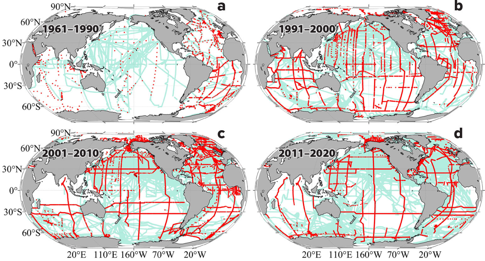
FIGURE 1. Sampling locations of autonomous fCO2 measurements (SOCATv2022, cyan) and discrete dissolved inorganic carbon, total alkalinity, or pH measurement (GLODAPv2.2022 and CODP-NA, red) during four intervals: (a) 1961–1990, (b) 1991–2000, (c) 2001–2010, and (d) 2011–2020. > High res figure

 

Analytical Methods

This analysis used ocean carbon data from SOCAT (version 2022, 1957–2021; Bakker et al., 2016), the 2002 update to the Global Ocean Data Analysis Project version 2 data product (GLODAPv2.2022, with measurements spanning 1972–2021; Lauvset et al., 2022), and the Common Online Data Analysis Platform in North America (CODAP-NA, version 2021, 2003–2018; Jiang et al., 2021). SOCAT provided the most comprehensive spatial coverage with approximately 34 million surface fCO₂ observations (Figure 1). To examine the temporal changes, four time intervals with global coverage were identified. They are “1975” (covering 30 years of observations from 1961 to 1990), “1995” (covering 10 years of observations from 1991 to 2000), “2005” (covering observations from 2001 to 2010), and “2015” (covering observations from 2011 to 2020). In the initial time interval (1961–1990), observations from three decades were used to ensure there was sufficient information to derive a 1°×1° global map. A detailed description of the methods involved in the preparation of the maps is provided in the online Supplementary Materials.

The surface underway fCO₂ measurement system was developed by a team of scientists and engineers led by Denis Pierrot of AOML (Pierrot et al., 2009), improving on earlier designs by combining air-water equilibrators with an infrared analyzer for detection (Takahashi, 1961; Wanninkhof and Thoning, 1993; Feely et al., 1998). The system, which was designed to operate unattended onboard a ship, is composed of a “wet box” where seawater is equilibrated with air, and a dry box with a gas analyzer and a computer interface that are generally located side-by-side on a wall near a sink and drain (Figure 2). The system operates by directing a continuous flow of surface seawater through a showerhead chamber (the equilibrator) where the CO₂ contained in the seawater equilibrates with the gas present in the chamber. The gas within is periodically pumped through a non-dispersive Licor infrared analyzer that measures the gas CO₂ mole fraction (xCO₂), and is then returned to the equilibrator. At specified time intervals, atmospheric air is also pumped through the analyzer, and its CO₂ mole fraction is measured. The analyzer is calibrated with four CO₂ standard gases that are prepared by the NOAA Global Monitoring Laboratory and are traceable to the World Meteorological Organization scale. The system can run unattended for months at a time with only periodic maintenance and can transmit its data daily via satellite communication, thus allowing near-real-time data analysis and remote troubleshooting.

 

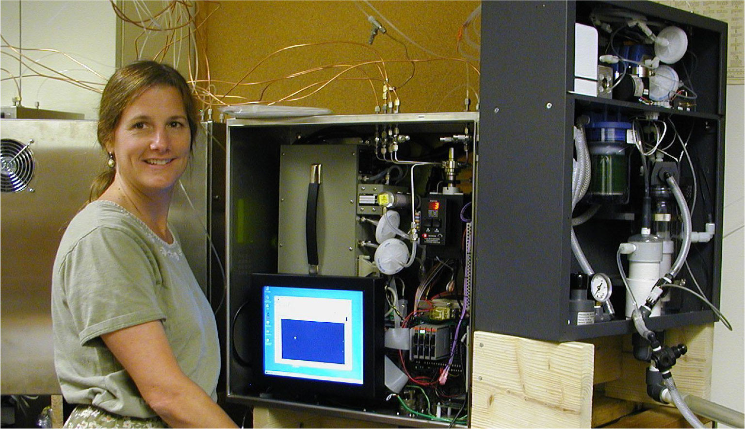
FIGURE 2. The NOAA Pacific Marine Environmental Laboratory (PMEL) underway fCO2 system, originally designed by Craig Neill, is a two-box measuring system ( “dry box” at left, “wet box” at right), being maintained here by Cathy Cosca of PMEL. > High res figure

 

For this study, the distribution of surface ocean hydrogen ion content and the aragonite saturation state are derived from gridded global observations of seawater fCO₂ and salinity following the approach described in Jiang et al. (2019) and averaged for four data intervals: 1960–1989, 1990–1999, 2000–2009, and 2010–2019. This calculation employs the strong correlation between fCO₂ and [H⁺] that is given by the relationship

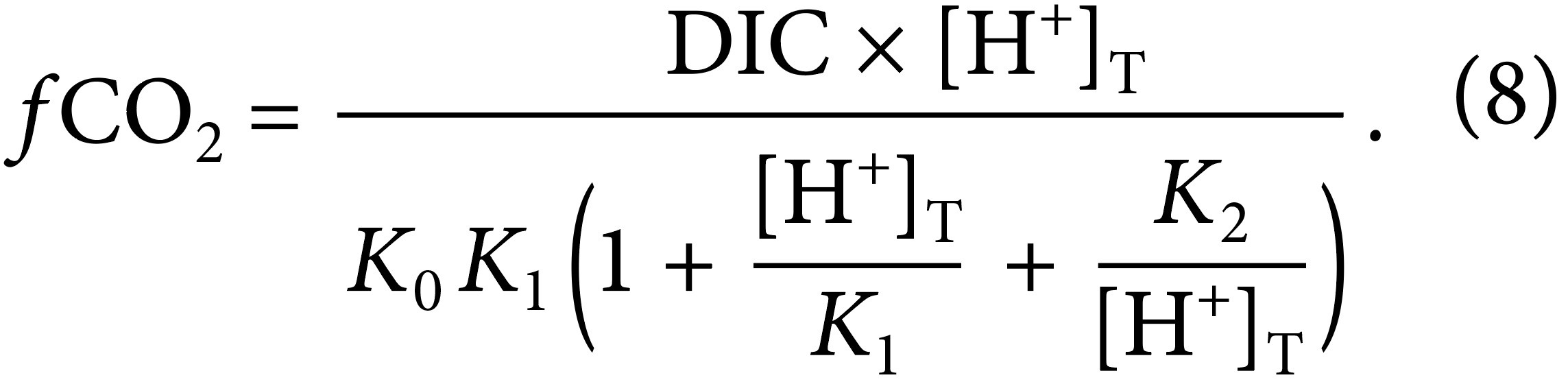
The term on the right-hand side of the equation in parentheses exhibits a dependence on [H⁺]_T (on the total hydrogen ion scale), and thus fCO₂ and [H⁺]_T are nearly directly proportional. We used the most recent SOCATv2022 fCO₂ data to calculate [H⁺]_T.

There is also a strong correlation between total A_T and salinity (Lee et al., 2006) in surface waters that allows A_T to be estimated with reasonable skill even when only measurements of salinity are available. We therefore use the updated A_T and DIC empirical seawater estimation routines of Carter et al. (2021) to calculate the aragonite and calcite saturation states in surface water by employing the equations for K_sp given by Mucci (1983).

The model outputs are from a model-​data fusion product that was created by combining 14 Earth System Models from the latest Coupled Model Intercompari­son Project Phase 6 (CMIP6) with three recent observational ocean carbon data products (Jiang et al., 2023). The temporal evolution of surface OA indicators as decadal averages—ranging from historical conditions (1850–2010) to two future shared socioeconomic pathways (2020–2100): SSP1-1.9 and SSP5-8.5—was used as a reference for the observational data-based temporal changes.

 

Results

fCO₂ and CO₃^2– Distributions

Figure 3 shows the global average fCO₂ and CO₃^2– distributions for four time intervals—​1961–1990, 1991–2000, 2001–2010, and 2011–2020. The fCO₂ values were obtained from surface measurements and the CO₃^2– distributions from calculations using the algorithms of Carter et al. (2021). Surface ocean fCO₂ values are generally highest across all time intervals in tropical, subtropical, and coastal upwelling zones (>400 µatm) where upwelling is strongest and/or surface seawater temperatures were also highest (Figure 3a). The lowest values are generally observed at higher latitudes (<360 µatm), where surface water temperatures are at a minimum. Even though water fCO₂ generally tends to increase over time everywhere, the horizontal gradients in fCO₂ tend to increase particularly in the west-east direction. For example, the west-east fCO₂ increase along the equatorial Pacific grows by as much as 50–80 µatm over the span of the four time intervals. This increasing gradient in the surface waters is largely due to combined effects of the increasing CO₂ levels (Steinacher et al., 2009), increasing sea surface temperatures, decreasing buffer capacity of seawater (Fassbender et al., 2018; Feely et al., 2018; Jiang et al., 2019), and the effects of ice melt in the polar regions (Yamamoto et al., 2012; Carton et al., 2015; Qi et al., 2022). The increase of strong horizontal gradients is consistent with the model results that extend out to the year 2100 (Jiang et al., 2019, 2023). Overall, surface fCO₂ increases average about 16 µatm per decade based on these observations.

 

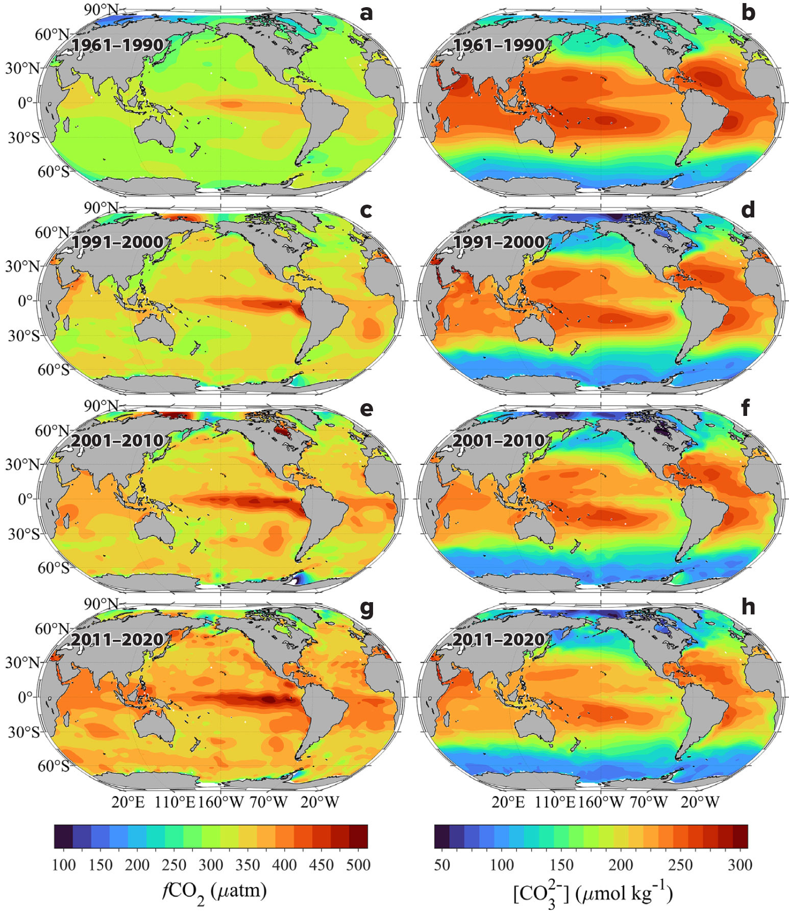
FIGURE 3. Distribution of (left) carbon dioxide fugacity (fCO2) and (right) carbonate ion content ([CO32–]) in surface waters for four intervals: (a,b) 1961–1990, (c,d) 1991–2000, (e,f) 2001–2010, and (g,h) 2011–2020. > High res figure

 

In contrast, Figure 3b shows surface water carbonate ion concentrations to be highest in the subtropics and lowest in high-latitude regions. They are also high on the western side of the subtropical regions where salinity and A_T are also highest. There are strong horizontal gradients in CO₃^2– concentrations that mimic the salinity distribution, indicating the high degree of correlation between surface water CO₃^2– and A_T (Jiang et al., 2023). CO₃^2– concentrations range from about 270 µmol kg^–1 in the subtropics to about 70 µmol kg^–1 in the high Arctic and Antarctic zones. Throughout the timeframe of the observations, surface water CO₃^2– concentrations decrease at a rate of approximately –5.1 µmol kg^–1 decade^–1, with the largest decreases (nearly 50%) occurring in the western subarctic regions compared with the subtropics and tropics. Nevertheless, large west-east gradients exist, the strongest in the Atlantic and Pacific basins and the weakest in the Indian Ocean. Similarly, sharp gradients exist across the major fronts in the north-south direction in all three major ocean basins. These gradients are primarily driven by the increasing CO₂ emissions to the atmosphere and the increasing sea surface temperature values toward the equator.

 

[H⁺]_T and pH_T Distributions

Surface ocean hydrogen ion content ([H⁺]_T) shows similar spatial distribution as fCO₂ because of their linear relationship (Equation 8). The averaged global surface ocean [H⁺]_T contents for the four intervals indicate significant regional and decadal variations (Figure 4). [H⁺]_T ranges between 5.2 and 10.5 nmol kg^–1, with the lowest values being in the high-​latitude regions of the Arctic and Southern Ocean waters and the highest values observed in the upwelling regions of the tropics, subtropics, and eastern boundary current regions. High values are also observed in the coastal upwelling regions and marginal seas (see Guo et al., 2022, and references therein). With each succeeding time period, the [H⁺]_T concentrations increase everywhere, particularly in the temperate and subpolar regions where [H⁺]_T concentrations increase by as much as 40%–50% over the total timespan of the measurements. In the region off northern Siberia, for example, [H⁺]_T concentrations increase nearly 50%, from 6.3 to 9.5 nmol kg^–1. Large increases also occur in the subtropical regions (~1–1.5 nmol kg^–1), particularly within the northern Indian Ocean and Gulf of Aden, the tropical seas off western Africa, and the Southern Ocean off Antarctica, especially in the Drake Passage. The smallest increases occur in the upwelling regions of the eastern equatorial Pacific where [H⁺]_T concentrations were already quite high (>8.1 nmol kg^–1). Low changes were also observed in the Greenland and Labrador Seas. Global area-averaged [H⁺]_T concentrations show an overall increase of approximately +0.3 nmol kg^–1 per decade, with higher rates of change occurring in the regions with the lowest observed initial concentration and the opposite at the higher concentrations (Figure 4). These results suggest an overall trend of increasing [H⁺]_T concentrations over the timeframe of the observations, consistent with ocean acidification.

 

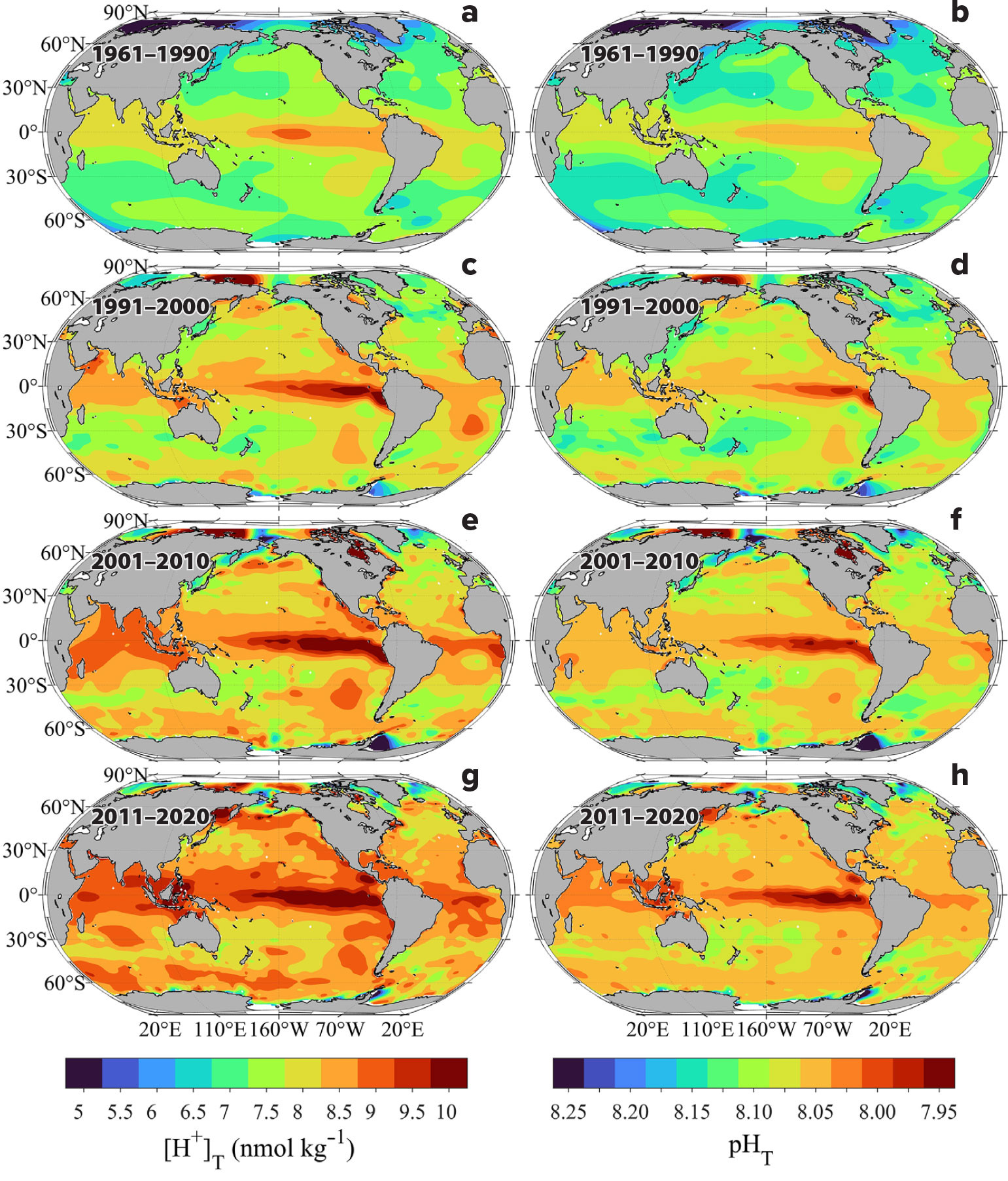
FIGURE 4. Distribution of (left) total hydrogen ion content ([H+]T) and (right) pH on total scale (pHT) in surface waters for four time intervals: (a,b) 1961–1990, (c,d) 1991–2000, (e,f) 2001–2010, and (g,h) 2011–2020. > High res figure

 

The pH_T distribution patterns indicate significant declines throughout the global ocean, with the most rapid changes occurring in the high-latitude polar and subpolar regions (Figure 4) where increasing CO₂ emissions and decreasing buffer capacity have the greatest overall impact (Fassbender et al., 2018; Feely et al., 2018; Qi et al., 2022; Jiang et al., 2023). Rapid pH_T declines are also observed in the western half of the northernmost and southernmost parts of the temperate regions because the gradients are large and subject to rapid declines in buffer capacity. The slowest rates of change occur in the tropics and subtropics where surface seawater temperatures are high and buffer capacity is also relatively stable and high. On a global scale, the decrease in pH_T averages about –0.016 per decade over the timeframe of the measurements, consistent with an earlier estimate of –0.018 per decade for the period between 1991 and 2011 (Lauvset et al., 2015).

 

Ω_ar and Ω_cal Distribution Patterns

Previous research by Mucci (1983) shows that aragonite is 50% more soluble than calcite and, consequently, surface water aragonite saturation state values will be approximately 50% lower than calcite. Aragonite saturation state values in surface waters mapped in Figure 5 generally range from about 1.5 to about 4.5 and are generally highest (>2.8) in the subtropics where the waters are warmest and most saline, and lowest (<2.5) in the polar and subpolar regions of the Northern and Southern Hemispheres. Low values (<2.5) are also found in the coastal upwelling regions along the west coasts of North America, South America, and Africa (Figure 5). There is also a strong west-to-east decreasing gradient in aragonite saturation state values in the equatorial Pacific due to strong upwelling in the eastern Pacific equatorial belt, which is also apparent to a much lesser extent in the Atlantic near the coast of West Africa. As with the [H⁺]_T concentrations, the strongest north-south gradients are observed near the boundaries between the subtropical and subpolar regions, particularly on the western side of the Pacific and Atlantic basins. Because surface seawater aragonite saturation state is a strong function of both seawater temperature and carbonate ion concentration, the steepest gradients roughly correspond to strong temperature and salinity fronts between subtropical and subpolar water masses in the northwestern Pacific and Atlantic Ocean basins. The gradients are smallest in the eastern boundary upwelling regions where the saturation state values are already low and more well mixed with the surrounding water masses. The global mean aragonite saturation state values for the surface ocean show an average decrease of approximately –0.08 per decade.

 

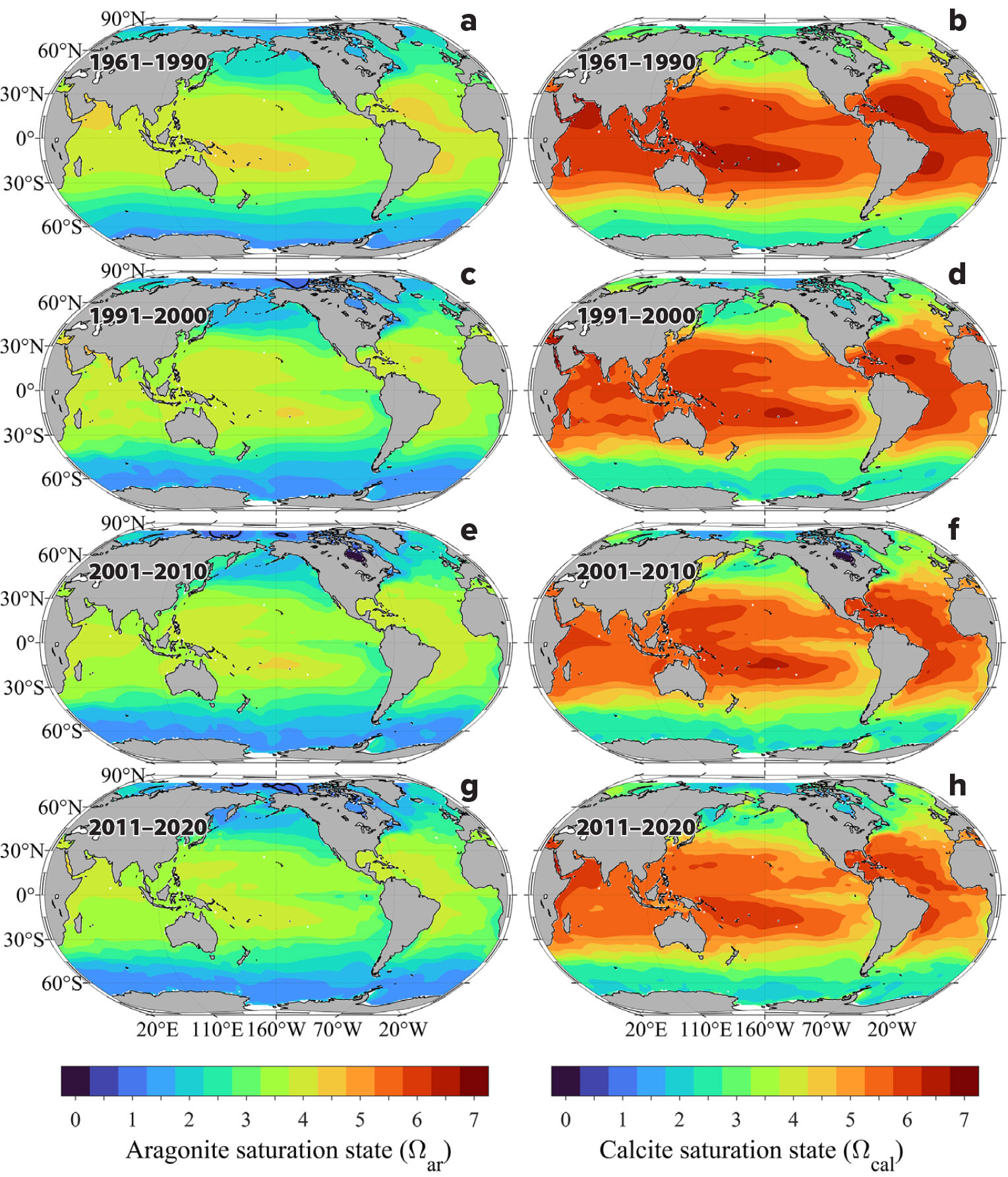
FIGURE 5. Distribution of (left) aragonite saturation state (Ωar) and (right) calcite saturation state (Ωcal) in surface waters for four time intervals: (a,b) 1961–1990, (c,d) 1991–2000, (e,f) 2001–2010, and (g,h) 2011–2020. > High res figure

 

The Ω_cal distribution patterns are very similar to the Ω_ar maps with the exception that the Ω_cal values are about 50% higher (Figure 5). The largest decreases in Ω_cal occur in the far western North Pacific near the boundary between the subtropical and subpolar regions, and the lowest rate of change occurs in the equatorial region. Over the duration of the measurements, Ω_cal values also decrease by approximately –0.12 per decade in surface waters, nearly identical to the aragonite saturation state rate of change.

 

Discussion

Comparisons with Model Outputs for Global Trends

Figure 6 shows the global ocean mean values of the surface observations along with corresponding model results for the shared socioeconomic pathway (SSP)1-1.9 CO₂ emission scenario (low emissions and high mitigation scenario, blue line) and the SSP5-8.5 scenario (high emissions and low mitigation scenario, red line; after Jiang et al., 2023). The global mean values for observations shown above the vertical columns represent the average values at the midpoint of each time interval. The results show very good agreement between the observations and the model outputs for the two CO₂ emission scenarios. The rates of change per decade are shown for each of the panels with significant increases in fCO₂ and [H⁺]_T and significant decreases in [CO₃^2–], pH_T, Ω_ar, and Ω_cal. The model scenarios show very similar values through 2020 for the two CO₂ emission scenarios. After that time, the model estimates for the two emission scenarios diverge sufficiently that observations should be able to delineate the differences, which could manifest within the next decade (Friedlingstein et al., 2022; Müller et al., 2023). The results indicate that under the SSP1-1.9 CO₂ emission scenario, the rate of change for each of the parameters will decrease, and under the SSP5-8.5 scenario, the rate of change will increase. These results suggest that the future trajectory of ocean acidification is highly dependent on which CO₂ emission scenario occurs in the future, with the ocean absorbing more CO₂ from the atmosphere under the SSP5-8.5 scenario and releasing it back to the atmosphere under the SSP1-1.9 CO₂ scenario. Continued monitoring and modeling of the carbon system parameters and pH will be critical for a clear understanding of the ocean’s chemistry and prediction of the sustainability of marine life in the rapidly changing conditions of the future.

 

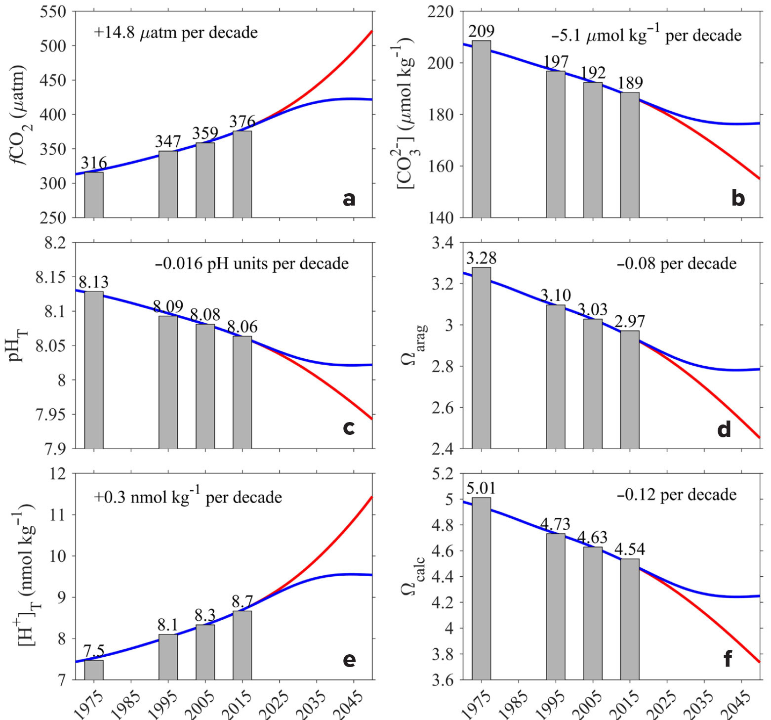
FIGURE 6. Global area-averaged (a) fCO2, (b) carbonate ion content, (c) pHT, (d) Ωar, (e) [H+]T, and (f) Ωcal from the GLODAPv2.2022 and SOCATv2022 surface ocean observational databases and associated model predictions for the time interval from 1970 through 2050. The blue line is the shared socioeconomic pathways (SSP)1-1.9 CO2 emission scenario, and the red line is the SSP5-8.5 scenario. > High res figure

 

Implications for Marine Calcifiers

Of the many conditions that are rapidly changing in the ocean, temperature, Ω_ar, pH, and oxygen concentrations are among the major abiotic drivers that interactively affect biological responses of marine organisms and define their vulnerability. Long-term OA trends from both observations and models indicate a gradual spreading of low Ω_ar waters that are approaching critical OA sensitivity thresholds in the upper ocean. Vertical and lateral gradients in Ω_ar appear to be decreasing in the ocean, corresponding to faster and more widespread rates of decline of suitable habitats even in regions that would normally be considered refugia. Shrinking Ω gradients are expected for two reasons. First, anthropogenic carbon enters the ocean through the air-sea interface; it is in the surface waters where anthropogenic carbon content and its impacts are greatest and where carbonate mineral saturation states are highest. Second, the carbonate ion itself allows for additional anthropogenic carbon uptake by neutralizing the carbonic acid produced by the hydration of CO₂, and therefore the areas with the highest natural CO₃^2– content tend to take up the most anthropogenic carbon for a given human-induced atmospheric fCO₂ increase. Such a loss of habitat refugia for pelagic calcifiers has important consequences for species distributions and persistence. Specifically, reduction of refuge areas limits the potential for population mixing and restocking from these regions to already impacted, poor-​quality habitats and adds sublethal stresses for calcifying individuals. The decline in availability of suitable habitat is especially problematic when multiple stressors occur together or in succession. For example, Bednaršek et al. (2022) suggest that the combined effects of unusually high temperatures caused by a marine heatwave in 2014–2015 immediately followed by a strong El Niño event and decreased aragonite saturation state in 2016 within the California Current Ecosystem may have caused the pelagic pteropod, Limacina helicina, to be absent from their normal habitat. These unfavorable conditions also prevented these regions from undergoing the normal population mixing and restocking from outside sources. As the optimal pteropod habitat continues to shrink through space and time, the frequency of the events related to species absence from their usual habitats could significantly increase, causing longer term concerns for population sustainability. With concurrent multistressor impacts of increasing temperature and decreasing Ω_ar and Ω_calc, we might also expect the distribution of some calcifying species to contract to a greater degree than implied by their thermal tolerance window or from aragonite saturation state threshold alone (Bednaršek et al., 2022).

 

Future Research

Because the ocean plays a major role in the global carbon cycle, there is a need to quantify the changing rates of CO₂ uptake across the air-sea interface and its transport into the ocean interior is growing. Thus, there is a strong need to enhance the suite of shipboard, moored, and autonomous CO₂, pH, and biological observations that provide the basis for global trend analysis and early warning regarding biological responses to multistressor events (IPCC, 2021, 2022; Friedlingstein et al., 2022). However, recent studies indicate that significant temporal data gaps still exist in some parts of our global observing system, particularly in the Southern Ocean where ships and moorings alone do not provide sufficient coverage to delineate seasonal and interannual trends (Gray et al., 2018; Keppler and Landschützer, 2019; Sutton et al., 2021). In this case, ship-based and moored observations will need to be augmented with uncrewed automated platforms that can collect and transmit high-quality carbon measurements in near-real time. Significant strides are being made using biogeochemical Argo floats for oxygen cycling measurements, and it is likely that biogeochemical Argo sensors for pH and nutrients will soon allow for meaningful improvements in the temporal resolution of ocean carbon inventory and flux estimates. These large-scale global surface and subsurface data sets can be utilized to track the changing rates of uptake and transport of carbon in the future ocean (Friedlingstein et al., 2022; Gruber et al., 2023), identify and evaluate the effectiveness of future marine carbon dioxide removal approaches (Cross et al., 2023), and delineate the ocean’s response to future mitigation strategies (IPCC, 2021). The carbon observations will also be very useful for validating global and regional models of ocean acidification over time, as well as for understanding biological impacts and potential feedbacks. Our results on multiple stressors suggest that building a multistressor framework for future field studies is essential for identifying the spatial and temporal domains over which multiple stressors co-occur, their severity and frequency, and the positive and negative drivers that could impact future ecosystems. Because of the potential for massive and rapid restructuring of populations and ecosystems, particular attention should be given to the inclusion of rapid extreme events within this multi­stressor framework.

 

Acknowledgments

The authors dedicate this paper to the many national and international scientists who contributed to the collection and quality control of the Surface Ocean CO₂ Atlas (SOCAT, version 2022), the Global Ocean Data Analysis Project Version 2 (GLODAPv2, version 2022), the Coastal Ocean Data Analysis Product in North America (CODAP-NA, version 2021), and the World Ocean Atlas 2018. We specifically want to express our most sincere appreciation to Dana Greeley, Julian Herndon, Andrew Collins, David Wisegarver, Geoff Lebon, Robert Castle, Denis Pierrot, Kevin Sullivan, Kitack Lee, and Geun-Ha Park. Funding for L-QJ was from the NOAA Ocean Acidification Program (OAP, Project ID: 21047) NOAA National Centers for Environmental Information (NCEI) through a NOAA Cooperative Institute for Satellite Earth System Studies (CISESS) grant (NA19NES4320002) at the Earth System Science Interdisciplinary Center (ESSIC), University of Maryland. BRC, SRA, and RAF thank NOAA’s Global Ocean Monitoring and Observing and Ocean Acidification Programs (GOMO Fund Reference Number 100018302, and OAP NRDD 20848, and award number NA210AR4310251) through the Cooperative Institute for Climate, Ocean, and Ecosystem Studies (CICOES) under NOAA Cooperative Agreement NA20OAR4320271, Contribution No. 2022-2012. RAF and SRA were by also supported by PMEL. NB acknowledges support from the Slovene Research Agency (ARRS “Biomarkers of subcellular stress in the Northern Adriatic under global environmental change,” project # J12468), as well as NOAA’s Multistressor project (project number NA22NOS4780171). This is PMEL Contribution number 5481.

Feely, R.A., L.-Q. Jiang, R. Wanninkhof, B.R. Carter, S.R. Alin, N. Bednaršek, and C.E. Cosca. 2023. Acidification of the global surface ocean: What we have learned from observations. Oceanography 36(2–3):120–129, https://doi.org/10.5670/oceanog.2023.222.

> Data Synthesis Methods (63 KB pdf)

Bakker, D.C.E., B. Pfeil, C.S. Landa, N. Metzl, K.M. O’Brien, A. Olsen, K. Smith, C. Cosca, S. Harasawa, S.D. Jones, and others. 2016. A multi-​decade record of high quality fCO₂ data in version 3 of the Surface Ocean CO₂ Atlas (SOCAT). Earth System Science Data 8:383–413, https://doi.org/​10.5194/​essd-8-383-2016.

Bednaršek, N., R.A. Feely, J.C.P. Reum, W. Peterson, J. Menkel, S.R. Alin, and B. Hales. 2014. Limacina helicina shell dissolution as an indicator of declining habitat suitability due to ocean acidification in the California Current Ecosystem. Proceedings of the Royal Society B 281:20140123, https://doi.org/​10.1098/rspb.2014.0123.

Bednaršek, N., C.J. Harvey, I.C. Kaplan, R.A. Feely, and J. Mozina. 2016. Pteropods on the edge: Cumulative effects of ocean acidification, warming, and deoxygenation. Progress in Oceanography 145:1–24, https://doi.org/10.1016/j.pocean.2016.04.002.

Bednaršek, N., R.A. Feely, N. Tolimieri, A.J. Hermann, S.A. Siedlecki, G.G. Waldbusser, P. McElhany, S.R. Alin, T. Klinger, B. Moore-Maley, and H.O. Pörtner. 2017. Exposure history determines pteropod vulnerability to ocean acidification along the US West Coast. Scientific Reports 7:4526, https://doi.org/10.1038/s41598-017-03934-z.

Bednaršek, N., R.A. Feely, E.L. Howes, B.P.V. Hunt, F. Kessouri, P. León, S. Lischka, A.E. Maas, K. McLaughlin, N.P. Nezlin, and others. 2019. Systematic review and meta-analysis toward synthesis of thresholds of ocean acidification impacts on calcifying pteropods and interactions with warming. Frontiers in Marine Science 6:227, https://doi.org/​10.3389/fmars.2019.00227.

Bednaršek, N., R.A. Feely, M.W. Beck, S.R. Alin, S.A. Siedlecki, P. Calosi, E.L. Norton, C. Saenger, J. Štrus, D. Greeley, and others. 2020. Exoskeleton dissolution with mechanoreceptor damage in larval Dungeness crab related to severity of present-day ocean acidification vertical gradients. Science of the Total Environment 716:136610, https://doi.org/​10.1016/j.scitotenv.2020.136610.

Bednaršek, N., P. Calosi, R.A. Feely, R. Ambrose, M. Byrne, K.Y.K. Chan, S. Dupont, J.L. Padilla- Gamiño, J.I. Spicer, F. Kessouri, and others. 2021. Synthesis of thresholds of ocean acidification impacts on echinoderms. Frontiers in Marine Science 8:602601, https://doi.org/10.3389/fmars.2021.602601.

Bednaršek, N., B.R. Carter, R.M. McCabe, R.A. Feely, E. Howard, F. Chavez, M. Elliott, J.L. Fisher, J. Jahncke, and Z. Siegrist. 2022. Pelagic calcifiers face increased mortality and habitat loss with warming and ocean acidification. Ecological Applications 32(7):e2674, https://doi.org/10.1002/eap.2674.

Carter, B.R., H.C. Bittig, A.J. Fassbender, J.D. Sharp, Y. Takeshita, Y.-Y. Xu, M. Álvarez, R.H. Wanninkhof, R.A. Feely, and L. Barbero. 2021. New and updated global empirical seawater property estimation routines. Limnology and Oceanography Methods 19(12):785–809, https://doi.org/10.1002/lom3.10461.

Carton, J.A., Y. Ding, and K.R. Arrigo. 2015. The seasonal cycle of the Arctic Ocean under climate change. Geophysical Research Letters 42(18):7,681–7,686, https://doi.org/​10.1002/2015gl064514.

Cross, J.N., C. Sweeney, E.B. Jewett, R.A. Feely, P. McElhany, B. Carter, T. Stein, G.D. Kitch, and D.K. Gledhill. 2023. Strategy for NOAA Carbon Dioxide Removal Research: A White Paper Documenting a Potential NOAA CDR Science Strategy as an Element of NOAA’s Climate Interventions Portfolio. NOAA Special Report. Washington, DC, 81 pp.

DeVries, T. 2022. The ocean carbon cycle. Annual Review of Environment and Resources 47(1):317–341, https://doi.org/​10.1146/annurev-environ-120920-111307.

Doney, S.C., D.S. Busch, S.R. Cooley, and K.J. Kroeker. 2020. The impacts of ocean acidification on marine ecosystems and reliant human communities. Annual Review of Environment and Resources 45:83–112, https://doi.org/10.1146/annurev-environ-012320-083019.

Fassbender, A.J., K.B. Rodgers, H.I. Palevsky, and C.L. Sabine. 2018. Seasonal asymmetry in the evolution of surface ocean pCO₂ and pH thermodynamic drivers and the influence on sea-air CO₂ flux. Global Biogeochemical Cycles 32(10):1,476–1,497, https://doi.org/​10.1029/2017GB005855.

Feely, R.A., R. Wanninkhof, H.B. Milburn, C.E. Cosca, M. Stapp, and P.P. Murphy. 1998. A new automated underway system for making high precision pCO₂ measurements aboard ships of opportunity. Pp. 92–103 in Proceedings of the Marc’h Mor Workshop, IUEM, Brest, France, November 17–19, 1997.

Feely, R.A., C.L. Sabine, K. Lee, F.J. Millero, M.F. Lamb, D. Greeley, J.L. Bullister, R.M. Key, T.-H. Peng, A. Kozyr, and others. 2002. In situ calcium carbonate dissolution in the Pacific Ocean. Global Biogeochemical Cycles 16(4):1144, https://doi.org/​10.1029/2002GB001866.

Feely, R.A., C.L. Sabine, K. Lee, W. Berelson, J. Kleypas, V.J. Fabry, and F.J. Millero. 2004. Impact of anthropogenic CO₂ on the CaCO₃ system in the oceans. Science 305(5682):362–366, https://doi.org/​10.1126/​science.1097329.

Feely, R.A., S. Alin, B. Carter, N. Bednaršek, B. Hales, F. Chan, T.M. Hill, B. Gaylord, E. Sanford, R.H. Byrne, and others. 2016. Chemical and biological impacts of ocean acidification along the west coast of North America. Estuarine, Coastal, and Shelf Science 183(A):260–270, https://doi.org/10.1016/​j.ecss.2016.08.043.

Feely, R.A., R.R. Okazaki, W.-J. Cai, N. Bednaršek, S.R. Alin, R.H. Byrne, and A. Fassbender. 2018. The combined effects of acidification and hypoxia on pH and aragonite saturation in the coastal waters of the California Current Ecosystem and the northern Gulf of Mexico. Continental Shelf Research 152:50–60, https://doi.org/10.1016/j.csr.2017.11.002.

Fox, L., S. Stukins, T. Hill, and C.G. Miller. 2020. Quantifying the effect of anthropogenic climate change on calcifying plankton. Scientific Reports 10(1):1620, https://doi.org/10.1038/s41598-020-58501-w.

Friedlingstein, P., M. O’Sullivan, M.W. Jones, R.M. Andrew, J. Hauck, A. Olsen, G.P. Peters, W. Peters, J. Pongratz, S. Sitch, and others. 2020. Global Carbon Budget 2020. Earth System Science Data 12:3,269–3,340, https://doi.org/10.5194/essd-12-3269-2020.

Friedlingstein, P., M.W. Jones, M. O’Sullivan, R.M. Andrew, D.C.E. Bakker, J. Hauck, C. Le Quéré, G.P. Peters, W. Peters, J. Pongratz, and others. 2022. Global Carbon Budget 2021. Earth System Science Data 14(4):1,917–2,005, https://doi.org/​10.5194/​essd-14-1917-2022.

Gattuso, J.-P., A. Magnan, R. Billé, W.W.L. Cheung, E.L. Howes, F. Joos, D. Allemand, L. Bopp, S.R. Cooley, C.M. Eakin, and others. 2015. Contrasting futures for ocean and society from different anthropogenic CO₂ emission scenarios. Science 349(6243), https://doi.org/10.1126/​science.aac4722.

Gray, A.R., K.S. Johnson, S.M. Bushinsky, S.C. Riser, J.L. Russell, L.D. Talley, R. Wanninkhof, N.L. Williams, and J.L. Sarmiento. 2018. Autonomous biogeochemical floats detect significant carbon dioxide outgassing in the high-latitude Southern Ocean. Geophysical Research Letters 45(17):9,049–9,057, https://doi.org/10.1029/2018GL078013.

Gruber, N., D. Clement, B.R. Carter, R.A. Feely, S. van Heuven, M. Hoppema, M. Ishii, R.M. Key, A. Kozyr, S. Lauvset, and others. 2019. The oceanic sink for anthropogenic CO₂ from 1994 to 2007. Science 363(6432):1,193−1,199, https://doi.org/​10.1126/science.aau5153.

Gruber, N., D.C. Bakker, T. DeVries, L. Gregor, J. Hauck, P. Landschützer, G.A. McKinley, and J.D. Müller. 2023. Trends and variability in the ocean carbon sink. Nature Reviews Earth and Environment 4:119–134, https://doi.org/10.1038/s43017-022-00381-x.

Guo, X., N. Bednaršek, H. Wang, R.A. Feely, and A. Laurent. 2022. Editorial: Acidification and hypoxia in marginal seas. Frontiers in Marine Science 9:861850, https://doi.org/10.3389/fmars.2022.861850.

IPCC. 2013. Climate Change 2013: The Physical Science Basis. Contributions of Working Group I to the Fifth Assessment Report of the Intergovernmental Panel on Climate Change. T.F. Stocker, D. Qin, G.-K. Plattner, M. Tignor, S.K. Allen, J. Boschung, A. Nauels, Y. Xia, V. Bex and P.M. Midgley, eds, Cambridge University Press, Cambridge, UK, and New York, NY, USA.

IPCC. 2021. Climate Change 2021: The Physical Science Basis. Contribution of Working Group I to the Sixth Assessment Report of the Intergovernmental Panel on Climate Change. V. Masson-Delmotte, P. Zhai, A. Pirani, S.L. Connors, C. Péan, S. Berger, N. Caud, Y. Chen, L. Goldfarb, M.I. Gomis, and others, eds, Cambridge University Press, Cambridge, UK, and New York, NY, USA, 2,391 pp., https://doi.org/10.1017/9781009157896.

IPCC. 2022. Climate Change 2022: Impacts, Adaptation, and Vulnerability. Contribution of Working Group II to the Sixth Assessment Report of the Intergovernmental Panel on Climate Change. H.-O. Pörtner, D.C. Roberts, M. Tignor, E.S. Poloczanska, K. Mintenbeck, A. Alegría, M. Craig, S. Langsdorf, S. Löschke, V. Möller, and others, eds, Cambridge University Press, Cambridge, UK, and New York, NY, USA.

Jiang, L.-Q., R.A. Feely, B.R. Carter, D.J. Greeley, D.K. Gledhill, and K.M. Arzayus. 2015. Climatological distribution of aragonite saturation state in the global oceans. Global Biogeochemical Cycles 29(10):1,656–1,673, https://doi.org/​10.1002/2015GB005198.

Jiang, L.-Q., B.R. Carter, R.A. Feely, S.K. Lauvset, and A. Olsen. 2019. Surface ocean pH and buffer capacity: Past, present and future. Scientific Reports 9:18624, https://doi.org/10.1038/s41598-019-55039-4.

Jiang, L.-Q., D. Pierrot, R. Wanninkhof, R.A. Feely, B. Tilbrook, S.R. Alin, L. Barbero, R.H. Byrne, B.R. Carter, A.G. Dickson, and others. 2021. Best practice data standards for discrete chemical oceanographic observations. Frontiers in Marine Science 8:705638, https://doi.org/10.3389/fmars.2021.705638.

Jiang, L.-Q., J. Dunne, B.R. Carter, J.F. Tjiputra, J. Terhaar, J.D. Sharp, A. Olsen, S. Alin, D.C.E. Bakker, R.A. Feely, and others. 2023. Global surface ocean acidification indicators from 1750 to 2100. Journal of Advances in Modeling Earth Systems 15(3):e2022MS003563, https://doi.org/​10.1029/2022MS003563.

Keppler, L., and P. Landschützer. 2019. Regional wind variability modulates the Southern Ocean carbon sink. Scientific Reports 9(1):7384, https://doi.org/​10.1038/s41598-019-43826-y.

Key, R.M., A. Kozyr, C.L. Sabine, K. Lee, R. Wanninkhof, J.L. Bullister, R.A. Feely, F.J. Millero, C.W. Mordy, and T.-H. Peng. 2004. A global ocean carbon climatology: Results from Global Data Analysis Project (GLODAP). Global Biogeochemical Cycles 18(4), https://doi.org/10.1029/2004GB002247.

Kroeker, K.J., R.L. Kordas, R. Crim, I.E. Hendriks, L. Ramajo, G.S. Singh, C.M. Duarte, and J.-P. Gattuso. 2013. Impacts of ocean acidification on marine organisms: Quantifying sensitivities and interaction with warming. Global Change Biology 19:1,884–1,896, https://doi.org/10.1111/gcb.12179.

Lauvset, S.K., N. Gruber, P. Landschützer, A. Olsen, and J. Tjiputra. 2015. Trends and drivers in global surface ocean pH over the past 3 decades, Biogeosciences 12:1,285–1,298, https://doi.org/​10.5194/bg-12-1285-2015.

Lauvset, S.K., N. Lange, T. Tanhua, H.C. Bittig, A. Olsen, A. Kozyr, S. Alin, M. Álvarez, K. Azetsu-Scott, S. Becker, and others. 2022. GLODAPv2.2022: The latest version of the global interior ocean biogeochemical data product. Earth System Science Data 14(12):5,543–5,572, https://doi.org/10.5194/essd-14-5543-2022.

Lee, K., L.T. Tong, F.J. Millero, C.L. Sabine, A.G. Dickson, C. Goyet, G.-H. Park, R. Wanninkhof, R.A. Feely, and R.M. Key. 2006. Global relationships of total alkalinity with salinity and temperature in surface waters of the world’s oceans. Geophysical Research Letters 33(19), https://doi.org/​10.1029/2006GL027207.

Le Quéré, C., R. Moriarty, R.M. Andrew, J.G. Canadell, S. Sitch, J.I. Korsbakken, G.P. Peters, R.J. Andres, T.A. Boden, P. Friedlingstein, and others. 2015. Global Carbon Budget 2015. Earth System Science Data 7:349–396, https://doi.org/10.5194/essd-7-349-2015.

Mucci, A. 1983. The solubility of calcite and aragonite in seawater at various salinities, temperatures, and one atmosphere total pressure. American Journal of Science 283:780–799.

Müller, J.D., N. Gruber, B. Carter, R. Feely, M. Ishii, N. Lange, S.K. Lauvset, A. Murata, A. Olsen, F.F. Pérez, and others. 2023. Decadal trends in the oceanic storage of anthropogenic carbon from 1994 to 2014. Science Advances 4(4):e2023AV000875, https://doi.org/10.1029/2023AV000875.

Orr, J.C., V.J. Fabry, O. Aumont, L. Bopp, S.C. Doney, R.A. Feely, A. Gnanadesikan, N. Gruber, A. Ishida, F. Joos, and others. 2005. Anthropogenic ocean acidification over the twenty-first century and its impact on calcifying organisms. Nature 437(7059):681–686, https://doi.org/10.1038/nature04095.

Osborne, E.B., R.C. Thunell, N. Gruber, R.A. Feely, and C.R. Benitez-Nelson. 2019. Decadal variability in twentieth-century ocean acidification in the California Current Ecosystem. Nature Geoscience 13:43–49, https://doi.org/10.1038/s41561-019-0499-z.

Osborne, E.B., E.B. Jewett, D.K. Gledhill, R.A. Feely, K. Osgood, K.M. Arzayus, J.M. Mintz, D.S. Busch, J. Tomczuk, and M.P. Acquafredda. 2020. National ocean, coastal, and Great Lakes region acidification research. Chapter 1 in NOAA Ocean, Coastal, and Great Lakes Acidification Research Plan: 2020–2029. E.B. Jewett, E.B. Osborne, K.M. Arzayus, K. Osgood, B.J. DeAngelo, and J.M. Mintz, eds, National Oceanic and Atmospheric Administration, US Department of Commerce, https://oceanacidification.​noaa.​gov/​ResearchPlan2020.aspx.

Pierrot, D., C. Neill, K. Sullivan, R. Castle, R. Wanninkhof, H. Lüger, T. Johannessen, A. Olsen, R.A. Feely, and C.E. Cosca. 2009. Recommendations for autonomous underway pCO₂ measuring systems and data-reduction routines. Deep Sea Research Part II 56(8–10):512–522, https://doi.org/10.1016/j.dsr2.2008.12.005.

Qi, D., Z. Ouyang, L. Cheng, Y. Wu, R. Lei, B. Chen, R.A. Feely, L.G. Anderson, W. Zhong, H. Lin, and others. 2022. Climate change drives rapid decadal acidification in the Arctic Ocean from 1994 to 2020. Science 377(6614):1,544–1,550, https://doi.org/​10.1126/science.abo0383.

Sabine, C.L., R.A. Feely, N. Gruber, R.M. Key, K. Lee, J.L. Bullister, R. Wanninkhof, C.S. Wong, D.W.R. Wallace, B. Tilbrook, and others. 2004. The oceanic sink for anthropogenic CO₂. Science 305(5682):367–371, https://doi.org/​10.1126/science.1097403.

Sabine, C.L., and R.A. Feely. 2007. The oceanic sink for carbon dioxide. Pp. 31–49 in Greenhouse Gas Sinks. D. Reay, N. Hewitt, J. Grace, and K. Smith, eds., CABI Publishing, Oxfordshire, UK.

Somero, G.N., J. Beers, F. Chan, T. Hill, T. Klinger, and S. Litvin. 2016. What changes in the carbonate system, oxygen, and temperature portend for the northeastern Pacific Ocean: A physiological perspective. Bioscience 66:14–26, https://doi.org/​10.1093/biosci/biv162.

Steinacher, M., F. Joos, T.L. Frölicher, G.-K. Plattner, and S.C. Doney. 2009. Imminent ocean acidification in the Arctic projected with the NCAR global coupled carbon cycle-climate model. Biogeosciences 6:515–533, https://doi.org/​10.5194/bg-6-515-2009.

Sutton, A.J., N.L. Williams, and B. Tilbrook. 2021. Constraining Southern Ocean CO₂ flux uncertainty using uncrewed surface vehicle observations. Geophysical Research Letters 48(3):e2020GL091748, https://doi.org/​10.1029/2020GL091748.

Takahashi, T. 1961. Carbon dioxide in the atmosphere and in Atlantic Ocean water. Journal of Geophysical Research 66:477–494, https://doi.org/10.1029/JZ066i002p00477.

Waldbusser, G.G., B. Hales, C.J. Langdon, B.A. Haley, P. Schrader, E.L. Brunner, M.W. Gray, C.A. Miller, and I. Gimenez. 2015. Saturation state sensitivity of marine bivalve larvae to ocean acidification. Nature Climate Change 5:273–280, https://doi.org/10.1038/nclimate2479.

Wanninkhof, R., and K. Thoning. 1993. Measurement of fugacity of CO₂ in surface water using continuous and discrete sampling methods. Marine Chemistry 44 (2–4):189–204, https://doi.org/​10.1016/0304-4203(93)90202-Y.

Yamamoto, A., M. Kawamiya, A. Ishida, Y. Yamanaka, and S. Watanabe. 2012. Impact of rapid sea-ice reduction in the Arctic Ocean on the rate of ocean acidification. Biogeosciences 9(6):2,365–2,375, https://doi.org/10.5194/bg-9-2365-2012.

Zeebe, R.E., and D.A. Wolf-Gladrow. 2001. CO₂ in Seawater: Equilibrium, Kinetics, Isotopes. Elsevier Science, Amsterdam, Netherlands, 367 pp.

This is an open access article made available under the terms of the Creative Commons Attribution 4.0 International License (https://creativecommons.org/licenses/by/4.0/), which permits use, sharing, adaptation, distribution, and reproduction in any medium or format as long as users cite the materials appropriately, provide a link to the Creative Commons license, and indicate the changes that were made to the original content. Images, animations, videos, or other third-party material used in articles are included in the Creative Commons license unless indicated otherwise in a credit line to the material. If the material is not included in the article’s Creative Commons license, users will need to obtain permission directly from the license holder to reproduce the material.