Worldwide, marine protected areas (MPAs) are increasingly created to protect and restore selected parts of the ocean and to enhance recreation, fishing, and sustainable resources. However, this process has outpaced the development and implementation of methods for assessing and monitoring these habitats. Here, we combine data from an echosounder, a conductivity-temperature-depth probe, and underwater cameras to efficiently survey El Bajo Espíritu Santo Seamount, located in the southwest Gulf of California, Mexico. Results include a bathymetric map detailing a ridge with three peaks; oceanographic profiles showing a 35 m deep mixed layer and anoxic conditions below 200 m; mean target strength estimates for Pacific creolefish, Paranthias colonus (–34.8 dB re 1 m², for mean total length ~33 cm), and finescale triggerfish, Balistes polylepis (–39.8 dB re 1 m², 38 cm); baseline estimates of biomass for both species (55.7 t, 95% CI = 30.3–81.2 t and 38.9 t, 95% CI = 21.1–56.6 t, respectively) found only in the oxygenated water near the top of the seamount; and indications that these reef fishes grazed on zooplankton in the mixed layer. We conclude that acoustic-​optical sampling is a practical approach for obtaining baseline information on MPAs and to efficiently monitor changes resulting from natural and anthropogenic processes.

Some fish species observed at El Bajo Espíritu Santo Seamount are typical of rocky reefs in the Gulf of California. The larger blue fish are king angelfish (Holacanthus passer), and the smaller white fish are scissortail damselfish (Chromis atrilobata). Both species were presumed to be too close to the seabed to be sampled acoustically. > High res figure

INTRODUCTION

The creation of marine protected areas (MPAs) worldwide has outpaced the application of tools to monitor their marine resources and essential habitats and to preserve ecosystems to bolster fish production. Innovative approaches are needed to delineate and monitor MPAs using combined technologies to estimate fish abundances and distributions. The survey operations should simultaneously map and monitor other components of the MPA ecosystem, such as zooplankton, oceanographic features, and seabed habitat. Acoustic-optical surveys (e.g., Demer, 2012; Michaels et al., 2019; Demer et al., 2020), using widely available instruments and software, offer a practical solution. MPA waters might be surveyed periodically using a scientific echosounder, a conductivity-​temperature-​depth probe (CTD), and underwater cameras deployed on the CTD and by scuba divers. The results could include descriptions of the bathymetry, oceanographic habitat, distributions of zooplankton and fishes, determination of the dominant fish species, and estimates of their biomasses.

An example of such an MPA survey is one carried out at El Bajo Espíritu Santo Seamount (EBES). EBES is part of the MPA Parque Nacional Zona Marina del Archipielago de Espíritu Santo (PNZMAES), located in the southwest Gulf of California, Mexico, which together with other islands and protected areas in the region is a UNESCO World Heritage Site (https://whc.unesco.org/en/​list/​1182). In 2007, PNZMAES was granted protected status to conserve and protect its ecosystem, which is representative of islands in the Gulf of California (Secretaría de Medio Ambiente y Recursos Naturales, 2007). The MPA is delineated by two rectangles, one around the archipelago and a smaller one around EBES (Figure 1). While no-fishing areas are established within the larger rectangle, sportfishing and commercial fishing with handlines are permitted in most of the PNZMAES, which is the most productive area in the La Paz region (Hernández-Ortiz, 2013). From 2008 to 2009, 350 t to 500 t of fish were caught there (Comisión Nacional de Áreas Naturales Protegidas, 2014).

EBES is northeast of the Bay of La Paz, Baja California Sur, about 13 km north of the Espíritu Santo Archipelago (Figure 1). It is a submarine ridge ~2.5 km long and ~0.8 km wide that rises from 1,000 m to ~18 m depth. Spring-tide currents >0.5 m s^–1 can cause twin eddies >1 km diameter in the lee (Klimley et al., 2005). The area may also have cyclonic gyres, one observed with a 100 km diameter and an average west-periphery speed of 56 cm s^–1 (Emilsson and Alatorre, 1997). Mixing brings nutrients to the surface, promotes primary production, and aggregates plankton on the ridge. The biomasses of plankton and macrozooplankton exceed those at nearby sites (González-Armas et al., 2002; González-Rodríguez et al., 2018). This production attracts reef fishes, pelagic fishes, and other vertebrates to the seamount (Klimley et al., 2005) and makes EBES both ecologically and economically important (Klimley and Butler, 1988).

 

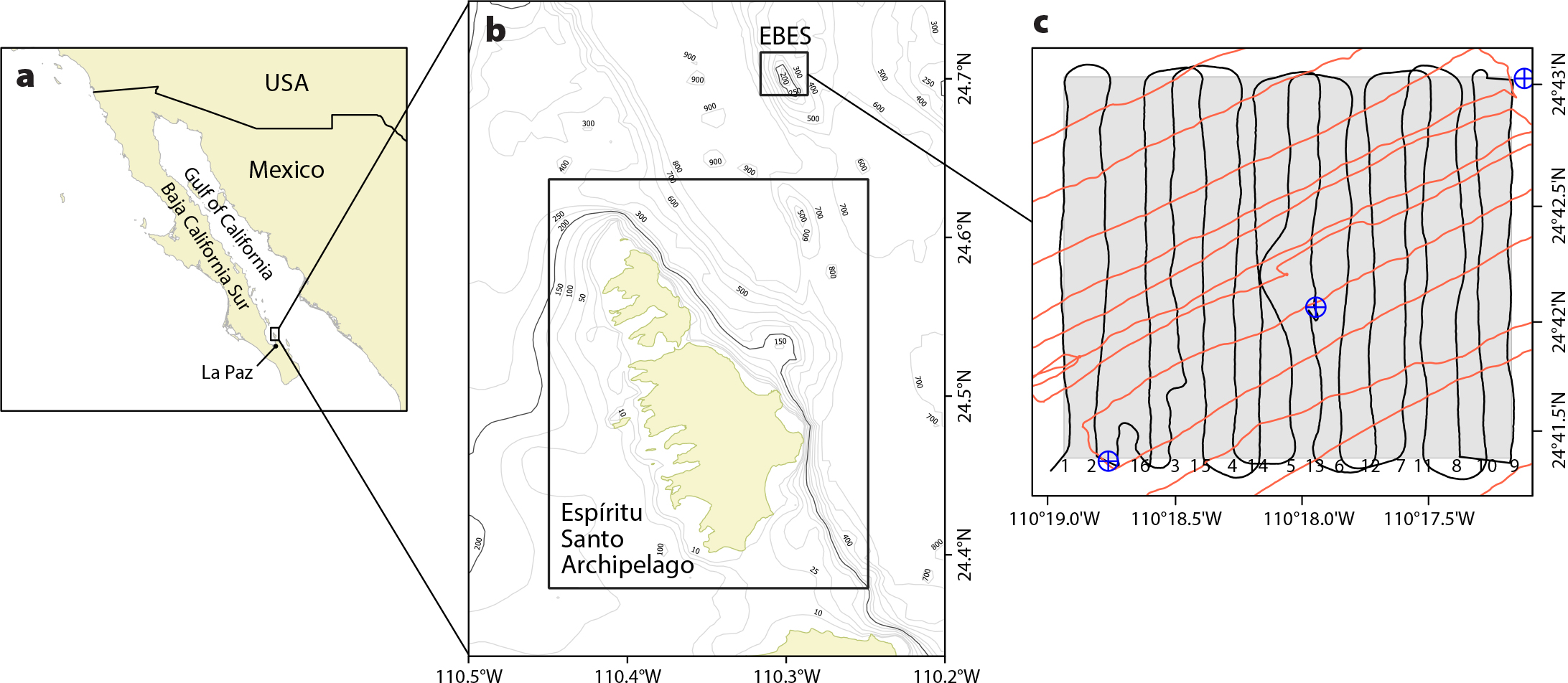
Figure 1. (a) Macrolocalization of the (b) Parque Nacional Zona Marina del Archipielago de Espíritu Santo (PNZMAES), with rectangles delineating the marine protected area (MPA), including the Espíritu Santo Archipelago and El Bajo Espíritu Santo Seamount (EBES). The coarse-scale bathymetry (GEBCO_2019) highlights the 200 m isobath (black). (c) At EBES, acoustic transects (black lines, numbered by transect) and CTD casts (blue symbols) were conducted on April 21, 2018. Red lines are acoustic sampling transects conducted on April 16, 2019. > High res figure

 

Transitions in the fish assemblage at EBES correspond with seasonal variations in the Gulf of California hydrography (Robles and Marinone, 1987). During winter conditions (water temperature 16°–20°C), pelagic fishes at the seamount include mostly yellowtail, amberjack, and red snapper; during summer conditions (24°–26°C), there are green jacks, hammerhead sharks, dolphinfish, and yellow snapper (Klimley et al., 2005).

Hammerhead sharks routinely congregate at EBES. A decline in their abundance (Klimley et al., 2005) corresponded to an increase in fishing for all hammerhead shark species worldwide during the past 50 years (Saldaña-Ruiz et al., 2017; Gallagher and Klimley, 2018), and the likely extirpation of some species from the Gulf of California (Pérez-Jiménez, 2014). With the depletion of larger fishes, the fisheries diversified (Erisman et al., 2010) and increasingly targeted Pacific creolefish (Paranthias colonus) and fine­scale triggerfish (Balistes polylepis) for human consumption rather than for fish bait (Sala et al., 2003). Between 1998 and 2012, catches of these species in the PNZMAES each averaged ~10 t yr^–1 (Hernández-Ortiz, 2013).

After more than a decade as an MPA, in November 2018 the PNZMAES became the first Mexican MPA to obtain the International Union for Conservation of Nature Green List Certificate, after meeting several criteria related to governance, design and planning, effective management, and conservation results (Ortega-Rubio et al., 2019). However, most of the monitoring efforts focus on the archipelago, and the status and recovery of the ecosystem at EBES have yet to be assessed and monitored. Here, we demonstrate a practical acoustic-optical surveying method and provide information that may be useful to researchers and managers. First, we describe the collection of echosounder data for mapping bathymetry and estimating the abundances of fish and zooplankton, as well as the collection of photographic images and video to identify fish species. Next, we present a map of the seamount and estimates of target strengths and biomass for Pacific creolefish and finescale triggerfish. Then we discuss these results in the context of local hydrographic conditions, in particular, the effect of dissolved oxygen on the vertical distribution of fish. Finally, we demonstrate how the integrated echosounder and optical sampling represents a cost-effective and practical approach for MPA monitoring.

 

METHODS

Overview

Acoustic sampling was executed along equally spaced transects spanning the EBES rectangle in April 2018 and April 2019, following the guidelines in Simmonds and McLennan (2005). The seabed and fish with gas-filled swimbladders created high-intensity echoes, indicating bathymetric features and fish-school locations, sizes, and densities, as described by Foote (1980). Plankton echoes were weaker but were of sufficient intensity to indicate their distribution and abundance, as in Hewitt and Demer (1991). The shapes of the fish and zooplankton aggregations, and bathymetric features, coupled with concurrently collected oceanographic information, allowed the separation and characterization of echoes from various taxa along the survey path. The identities of species contributing to the fish echoes were further refined using optical sampling with underwater cameras (e.g., Demer, 2012). The densities of the most abundant species were estimated by dividing their summed echo intensities by their average echo energy, estimated for representative animals (Simmonds and McLennan, 2005). Abundance was estimated by multiplying the average estimated fish density and the survey area. These steps are elaborated below.

 

Acoustic-Optical Survey

On April 21, 2018, the fishery research vessel BIP XII sampled 16 north-​south parallel-​line transects spaced 0.1 nmi apart spanning the rectangular 2.6 nmi² EBES area (Figure 1) at an average speed of 6.5 kt. The survey was conducted during daytime hours, ending at sunset, 19:46 MDT. Transects 1–9 progressed from west to east, from 12:07 to 15:15, then interstitial transects 10–16 progressed from east to west, from 15:52 to 17:55.

Along the transects, acoustic backscatter was measured with an echosounder (Simrad EK60) equipped with a 120 kHz split-beam transducer (Simrad ES120-7C) pole mounted port-side amidships, 3.19 m below the water surface. Measurements were made using 1,024 μs duration sound pulses transmitted every 0.65 s. The acoustic data were indexed with time (GMT), geographic position, and ship speed; bearing data were measured with a GPS receiver.

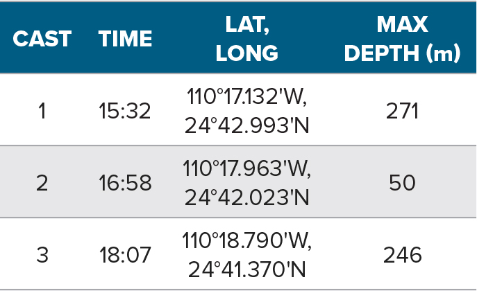
At the northeast and southwest corners and center of the study area, a probe (SBE 19plus) was deployed to measure seawater salinity (S), temperature (T, °C), and dissolved oxygen (O₂, mL L^–1) versus depth (Table 1).

 

Table 1. Time, location, and depth of CTD casts. > High res table

 

During Cast 2, near the top of the seamount, an underwater video camera (GoPro Hero 4 Black Edition) was attached to the probe and deployed to 50 m depth. To minimize potential reactions of fish to the probe, lights were not used. The images were examined to identify the species that contributed to the concomitantly measured acoustic backscatter.

On the top of the seamount (24°42.069'N, 110°18.052'W), five scuba divers collected underwater video and photographic images to identify and count fish species and observe their behaviors. The dives, to a maximum depth of 23.8 m, lasted 43 min with a “bottom time” of 36 min. The video cameras used during the dives were configured for 16 × 9 aspect, 1,920 × 1,080 pixels, 69.5° × 118.2° field of view, and 60 frames s^–1. To minimize potential reactions of fish to the divers, lights were used sparingly. Images were collected at depths ranging from 16.5 m to 23.8 m. The video-sampling distance, ~12–14 m, was limited by depth and water clarity. The photographic images (Nikon D500 camera and Sea & Sea DY-D2J strobes, 5600 K) provided detailed images with correct color to better identify fish species. The images also provided relative estimates of fish length. A 10 mm to 17 mm lens (Tokina) provided a 100° × 180° field of view. The sampling range, ~5–8 m, was limited by the strobe illumination.

Because BIP XII had to divert around the dive boat, the shallowest portion of EBES was not sampled with the 120 kHz echosounder. Therefore, on April 16, 2019, the mapping of bathymetry on the top of EBES was completed using an echosounder (Simrad EK80 Portable) with a 38 kHz transducer (ES38-18). The 6 m long boat surveyed 12 transects spaced 0.1 nmi to 0.2 nmi, oriented southwest to northeast (60°) and vice versa (240°) (Figure 1). The 1,024 μs pulses were transmitted every 1.5–0.25 s, depending on the seabed depth.

 

Bathymetric Mapping

The 120 kHz data were analyzed using commercial software (Echoview v8), and the 38 kHz data were processed using open-source software (ESP3 v1.2.1; Ladroit et al., 2020).

The mean temperature (14.7°C) and salinity (34.8) over 0 m to 280 m depth were used to estimate sound speed (1,525.24 m s^–1) (Fofonoff and Millard, 1983) and acoustic absorption at 120 kHz (0.048056 dB m^–1) and 38 kHz (0.006287 dB m^–1) (Francois and Garrison, 1982). The continuous noise power (≤–125 dB re 1 W) and transient noise were removed (details in De Robertis and Higginbottom, 2007; Ryan et al., 2015). For each transmission, the range to the seabed was estimated, indexed by date, time, and geographic position, and exported (.csv format).

The two bathymetry data sets were combined as overlapping data differed by <1 m. Depth contours were interpolated on a 50 m grid using ordinary kriging (geoR; Ribeiro and Diggle, 2018) in R (R Core Team, 2020).

 

Hydrographic Characterization

To obtain cross-sectional views of isolines spanning the area, the CTD data were interpolated using distances defined by variograms and correlograms. To identify the water masses present in the survey area, potential temperature and salinity versus depth were used to construct a T–S diagram. The anoxic depth was defined by a dissolved oxygen concentration of <0.5 mL L^–1 (Serrano, 2012).

 

Echo Classification

A –61 dB threshold on 120 kHz volume backscattering strength (S_v; dB re 1 m^–1) was used to classify the echoes as either zooplankton (≤ –61 dB) or fish (> –61 dB). The threshold was identified from iterative inspections of the distributions of S_v within polygons drawn around echoes from aggregations of putative fish and then zooplankton (Figure 2).

 

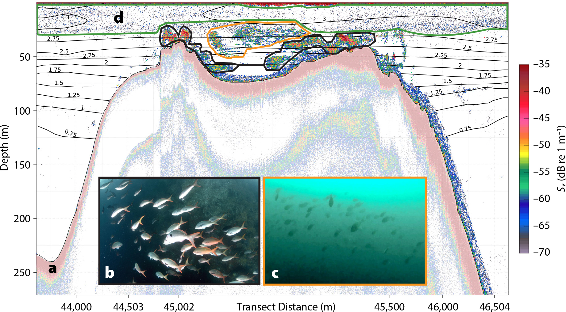
Figure 2. An example 120 kHz volume backscattering strength (Sv) echogram for transect 5 (see Figure 1 for location), showing echoes from: (a) the seabed (red band), (b) Paranthias colonus (inside the black line), (c) Balistes polylepis (inside the orange line), and (d) zooplankton (inside the green line). The plot is overlaid with isolines of dissolved oxygen concentration (mL L–1), calculated by Data-Interpolating Variational Analysis (Ocean Data View V.4; Schlitzer, 2015). > High res figure

 

To calculate the nautical area scattering coefficients (s_A; m² nmi^–2) for each taxon, the resulting zooplankton and fish echograms were each gridded into 3 m deep by 25 m long cells and depth-​integrated. Results were mapped, the former as interpolated contours (50 m grid) and the latter transformed to fish biomass (see Biomass Estimation below).

 

Target Strength Estimation

Using an algorithm with default parameters (Echoview), target strength (dB re 1 m²) measurements of individual fish were obtained from the 120 kHz data collected at the location and time of CTD Cast 2. The echogram and video images from this period indicated aggregations of two predominant species above the top of the seamount. Boundaries were drawn around the data (Figure 2) close to the seabed (identified as Paranthias colonus in the images) and farther above it (Balistes polylepis), and target strength values for these regions were exported separately. To determine whether the data from these regions were representative of fish atop other areas of the seamount, they were compared visually to the overall target strength distribution of single targets over the seamount. The mean target strength (TS) and corresponding mean backscattering cross sections (σ_bs = 10^TS/10) for the two principal species were calculated in the linear domain and assumed to be representative of all of the fish of the same species surveyed over the seamount.

 

Fish Mass Estimation

The distributions of total length (L_t; cm) for each species of fish observed during the survey were assumed to be similar to those captured by fisherman at EBES from 2011 through 2017 (unpublished data from Sociedad de Historia Natural Niparajá): for finescale triggerfish, root mean square total length (–L_t) was 38 cm (24 ≤ L_t ≤ 50 cm), and for Pacific creolefish, –L_t was 33 cm (26 ≤ L_t ≤ 40 cm). These lengths were converted to mass (m; g) using the equation m = 0.0547 L_t^2.66 for triggerfish (Barroso-Soto et al., 2007) and m = 0.0547 L_t^2.86333 for creolefish (Balart et al., 2006). The average mass per species is the arithmetic average of the individual mass estimates.

 

Biomass Estimation

For each grid cell, the s_A attributed to fish was apportioned to each of the two predominant species, Paranthias colonus and Balistes polylepis, using factors equal to the mean backscattering cross sections measured for each species, and the backscatter-​weighted proportion for that species, estimated from σ_bs and the number of each species observed in the video.

For grid cells within the 200 m isobath, fish densities by species (fish nmi^–2) were calculated by dividing the nautical area scattering coefficients by a factor equal to the corresponding individual backscattering cross section multiplied by 4π. Biomass densities (kg nmi^–2) for each species were calculated by multiplying these densities by the average-fish mass (kg fish^–1) for that species (Simmonds and MacLennan, 2005). These values, summed for both species and scaled to kg × 100 m⁻², were overlaid on a map of the depth contours and the interpolated zooplankton s_A. Total biomass (B; t) was calculated for each species by multiplying the mean fish biomass density (t nmi^–2) by the area (nmi²) within the 200 m isobath.

The variance of the fish nautical area scattering coefficient in the survey area was calculated using geostatistical methods implemented in Estimation Variance software (EVA; Petitgas and Prampart, 1995). A model was fit to the experimental variogram of the mean fish density, which was then used to compute the estimation variance of the mean biomass taking into account the geometry of the area, the length of the cell grid, the transect lengths, and the inter-transect distance (Petitgas, 1993). The standard error of the mean biomass was used to approximate the 95% confidence intervals (CIs) for the biomass.

 

RESULTS

Bathymetry

The bathymetry model for EBES indicates a shallow peak at ~25 m depth, and two deeper peaks at ~32 and ~43 m (Figure 3). To the west of the seamount the bottom depth exceeds 800 m, and to the east no more than 500 m. The ridge at the top of the seamount, defined here by the 200 m isobath, is about ~2.5 km long and ~0.8 km wide.

 

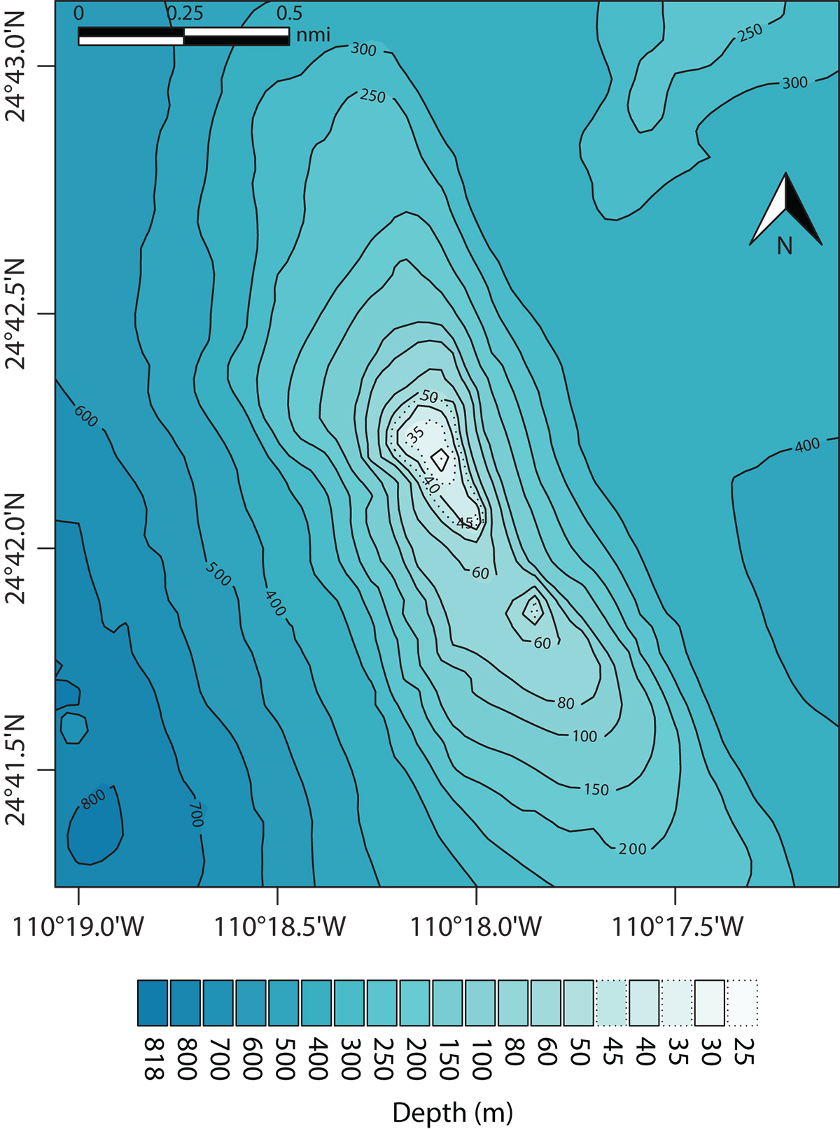
Figure 3. Bathymetry throughout the El Bajo Espíritu Santo MPA. The ridge has three peaks, consistent with measurements by Klimley et al. (2005). > High res figure

 

Oceanographic Environment

The CTD data indicate uniform conditions across EBES, with 34.6 < S < 35.3, 11° < T < 22.5°C, and 0.5 < O₂ < 3 mL L^–1. The highest values for the three variables were found in the upper mixed layer.

Across the study site, the surface mixed layer was ~35 m deep. A subsurface mixed layer, ~100 m to ~125 m depth, has S ~34.8, T ~14.5°C, and O₂ ~0.75 mL L^–1. Casts 1 and 3 indicate nearly anoxic conditions (0.54 mL L^–1 and 0.55 mL L^–1, respectively) at depths >200 m (Figure 4a).

During the survey, there were two predominant water-mass types at EBES (Figure 4b). Below the surface mixed layer, between ~25 m and ~70 m depths, the salty Gulf of California Water (GCW; S ≥ 34.9, T ≥ 12.0°C; Torres-Orozco, 1993) results from evaporation of Equatorial Surface Water (ESW). Between depths of ~70 m and ~250 m, Subtropical Subsurface Water (SSW; 34.5 < S < 35.0; 9.0° ≤ T ≤ 18°C; Torres-Orozco, 1993) originates from the Pacific Ocean (Castro et al., 2006).

 

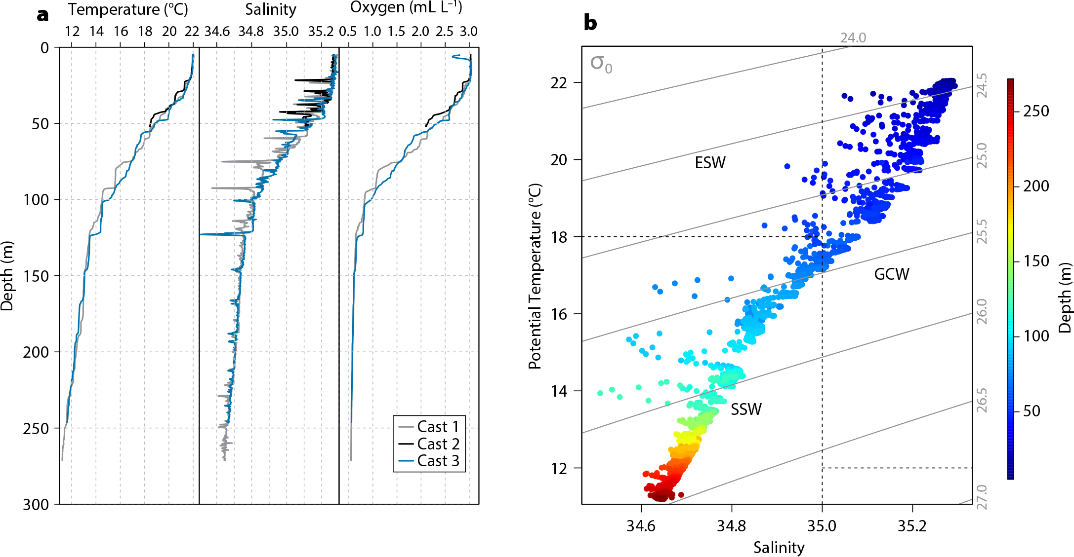
Figure 4. (a) Salinity, temperature, and dissolved oxygen versus depth at EBES, measured with three CTD casts conducted on April 21, 2018. The bottom of the mixed layer is at ~35 m depth, and the oxygen concentration is nearly anoxic (~0.5 mL L–1) below ~200 m depth. (b) Water masses present at EBES on April 21, 2018, included Gulf of California Water (GCW), indicated by S > 35 and T > 12°C, and Subtropical Subsurface Water (SSW), indicated by 100 m < D < 500 m, 34.5 < S < 35.0 and 9.0° < T < 18.0°C (Torres-Orozco, 1993; Amador-Buenrostro et al., 2003). Not observed, but potentially in the area, were Equatorial Surface Water (ESW) characterized by 0 m < D < 100 m, S < 35, and T > 18.0°C, and Pacific Intermediate Water (PIW) characterized by D > 500 m, 34.5 < S < 34.8, and 4.0° < T < 9.0°C (Amador-Buenrostro et al., 2003). > High res figure

 

Fish Species

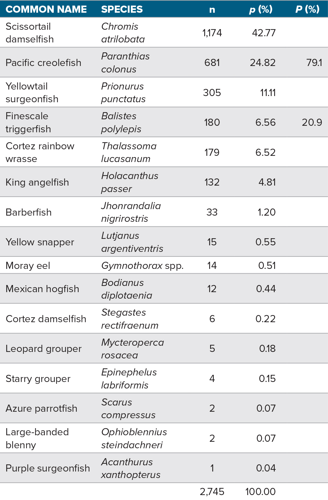
Images from just one camera were used for identifying and counting fish to avoid overlap with imagery collected by the other four divers. Fish counts by species were estimated from 122 images, one from each 15 s segment of video. From these images, a total of 16 fish species were identified (Table 2 and Figure 5). The predominant species observed in the video, and more clearly identified in the still images are: Scissortail damselfish (Chromis atrilobata), Pacific creole fish (Paranthias colonus), yellowtail surgeonfish (Prionurus punctatus), finescale triggerfish (Balistes polylepis), Cortez rainbow wrasse (Thalassoma lucasanum), and king angelfish (Holacanthus passer). Of these, P. colonus and B. polylepis accounted for 79.1% and 20.9% of the fish thought to be sufficiently above the seabed to be detected acoustically (see Demer et al., 2009). Though the fish were not measured, the still images taken during this study indicate that the B. polylepis were larger than the P. colonus.

 

Table 2. Number of individuals (n) and the species percentage observed (p) in 122 images. One image was extracted from each 15 s video segment collected during one scuba dive on the EBES seamount. Also indicated are the percentages of the two species that aggregated sufficiently above the reef to be sampled acoustically (P). > High res table

 

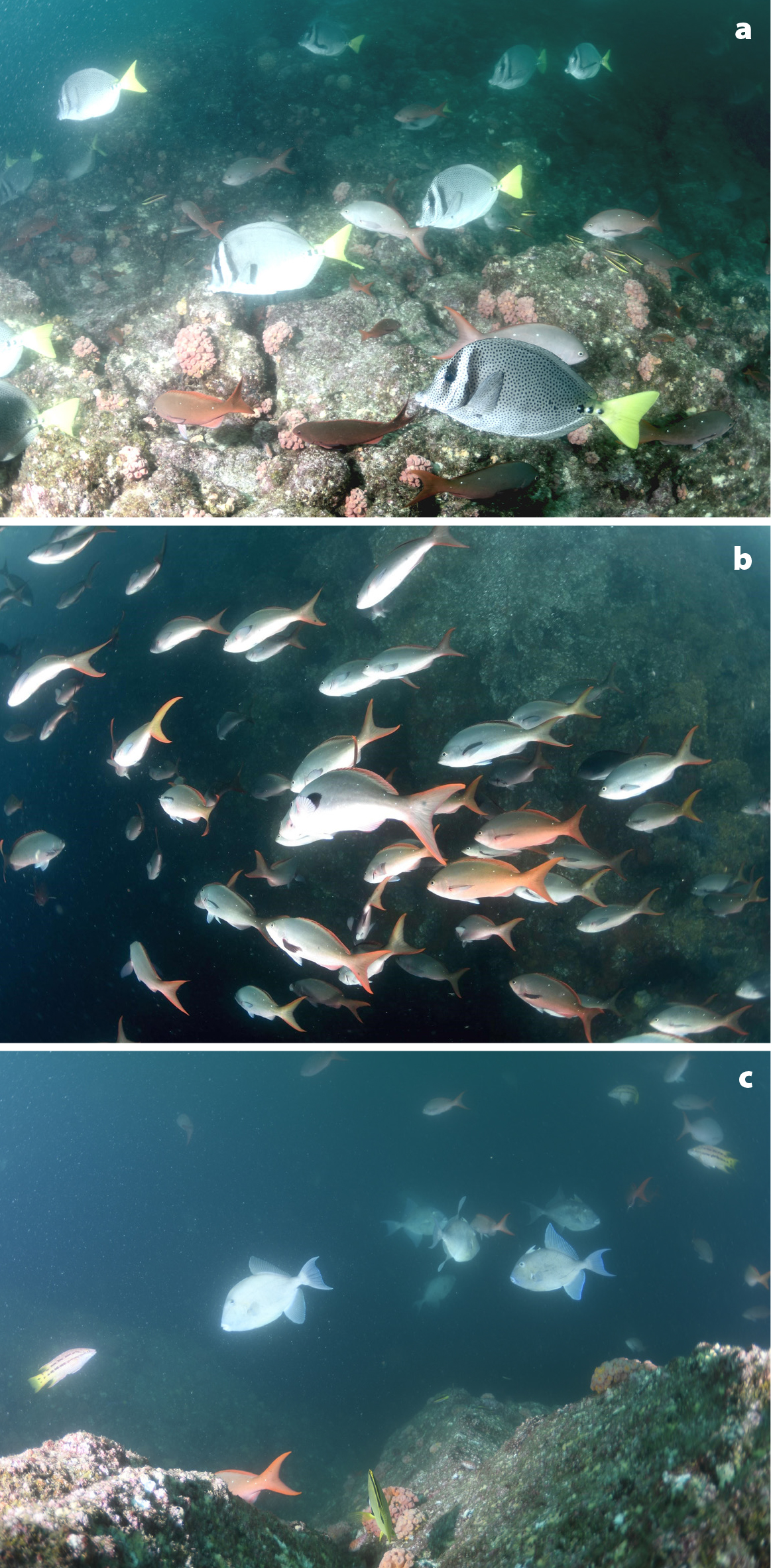
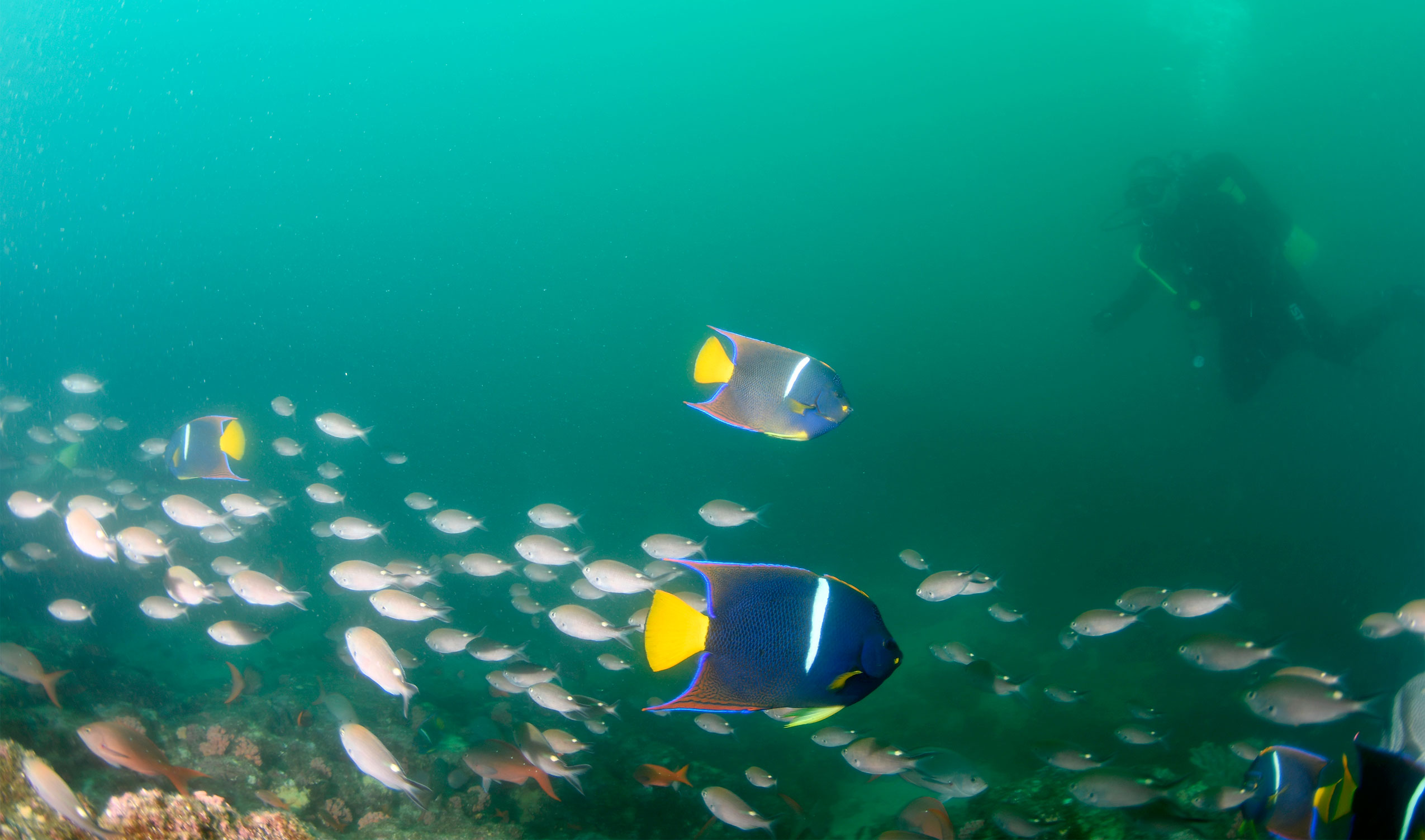
Figure 5. Some fish species observed at EBES are typical of rocky reefs in the Gulf of California. (a) Aggregations of yellowtail surgeonfish (Prionurus punctatus) were feeding near the seabed on top of the seamount. This species was also presumed to be too close to the seabed to be sampled acoustically. Pacific creole fish (Paranthias colonus), which were generally observed farther off the seabed, are also shown. (b) Pacific creole fish (Paranthias colonus; orange tails), seen here schooling above the seabed near the top of the seamount, were the most common pelagic species observed by divers. (c) Finescale triggerfish (Balistes polylepis; light color) were the second most common pelagic species observed by the divers. Mexican hogfish (Bodianus diplotaenia; black-spot stripes with yellow tail) were observed less frequently (see Table 2). > High res figure

 

Target Strength

The target strength distribution shown in Figure 6 largely includes measurements of individual Pacific creolefish and finescale triggerfish that were made throughout the survey. In addition, the distribution includes two small modes with higher values that may be from yellowtail surgeonfish (Prionurus punctatus) and king angelfish (Holacanthus passer), which were infrequently observed above the seabed (Table 2).

The mean target strength for in situ Pacific creolefish was –34.8 dB re 1 m² (σ_bs = 0.0003309 m²) (n = 141), assumed to correspond with –L_t = 33 cm; and for in situ finescale triggerfish, mean target strength = –39.8 dB re 1 m² (σ_bs = 0.0001038 m²; n = 238; –L_t = 38 cm) (Figure 6).

 

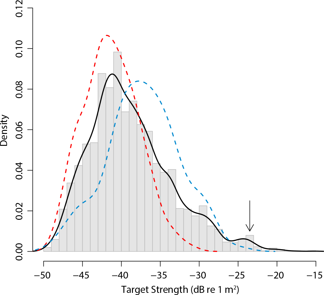
Figure 6. Distribution of target strengths (dB re 1 m2) measured from all resolvable individual fish detected above the seamount (gray bars) and a fit probability density distribution (black line) compared to target strength distributions for Pacific creolefish (blue line) and finescale triggerfish (red line) concomitantly observed acoustically and optically during the second CTD cast. Based on their behaviors and numbers observed by the divers, the small third and fourth modes at ~ –29 dB and ~ –23 dB (arrow) may be from yellowtail surgeonfish (Prionurus punctatus) and king angelfish (Holacanthus passer). > High res figure

 

Echo Classification and Biomass Estimation

The two dominant species of fish that were deemed sufficiently above the seabed to be detected acoustically were P. colonus (~79.1%) and B. polylepis (~20.9%) (Table 2). Both species were assumed to contribute all of the fish acoustic backscatter, nearly all of which (mean = 1,292 m² nmi^–2; maximum = 63,002 m² nmi^–2) was near the top of the seamount, at depths <200 m, in seawater with dissolved oxygen concentration >0.5 mL L^–1 (Figure 2). The fish backscatter outside of this polygon was negligible (mean = 3.7 m² nmi^–2, maximum = 461 m² nmi^–2). When converted to biomass, the maximum combined biomass densities were 23.15 t × 100 m^–2 (mean = 475 kg × 100 m^–2) inside the polygon, and 169 kg × 100 m^–2 (mean = 1.35 kg × 100^–2) in the remainder of the area. For the relatively oxygenated area within the 200 m isobath where most of the fish were observed, the estimates of total biomass are 55.7 t (95% CI = 30.3–81.2 t) for P. colonus (92% of total fish backscatter), and 38.9 t (95% CI = 21.1–56.6 t) for B. polylepis (8% of total fish backscatter) (Figure 7). The estimation variance was 95,021, and the coefficient of variation was 23.3%.

 

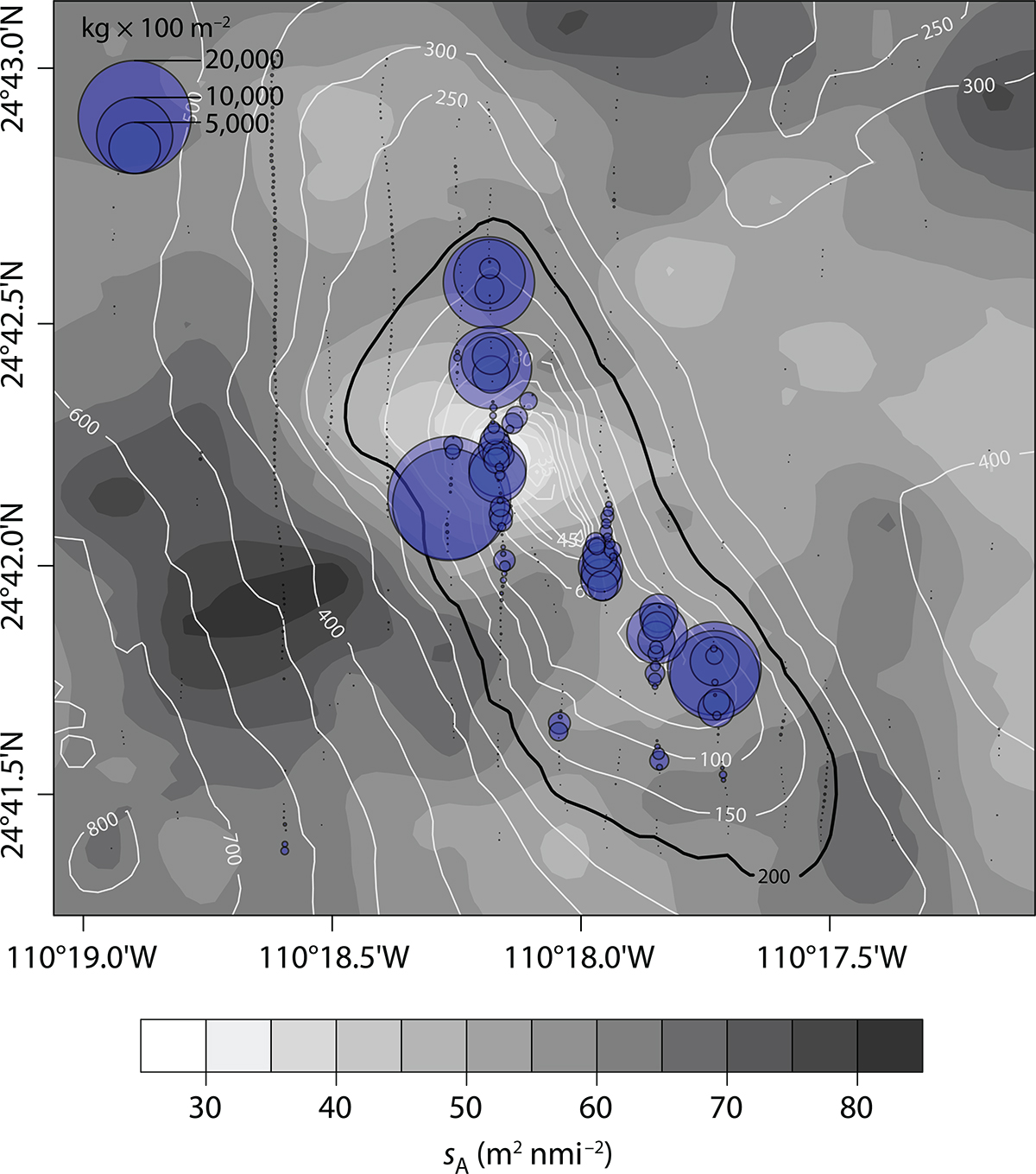
Figure 7. Distributions of fish biomass density (blue circles), equaling the sum of estimates for P. colonus and B. polylepis for 25 m distances along the survey transects, and interpolated zooplankton backscatter in the 35 m deep surface layer (gray contours) for transects 1–9 (see Figure 1 for transect locations). The 200 m isobath (black), delimiting the biomass-estimation area, is distinguished from the other isobaths (white). > High res figure

 

During the first pass, at midday, zooplankton backscatter was relatively homogeneously distributed throughout the MPA, mostly confined to the upper mixed layer (Figure 2), though it appeared to be lower above the top of the seamount (Figure 8a). Considering only transects 1–9, the mean and maximum zooplankton backscatter measures in the 35 m deep surface mixed layer were 58 m² nmi^–2 and 97 m² nmi^–2, respectively. In the second acoustic pass, late in the day (Figure 8b), plankton backscatter increased toward the west. This pattern is attributed to plankton migrating from deeper waters at the end of the day.

 

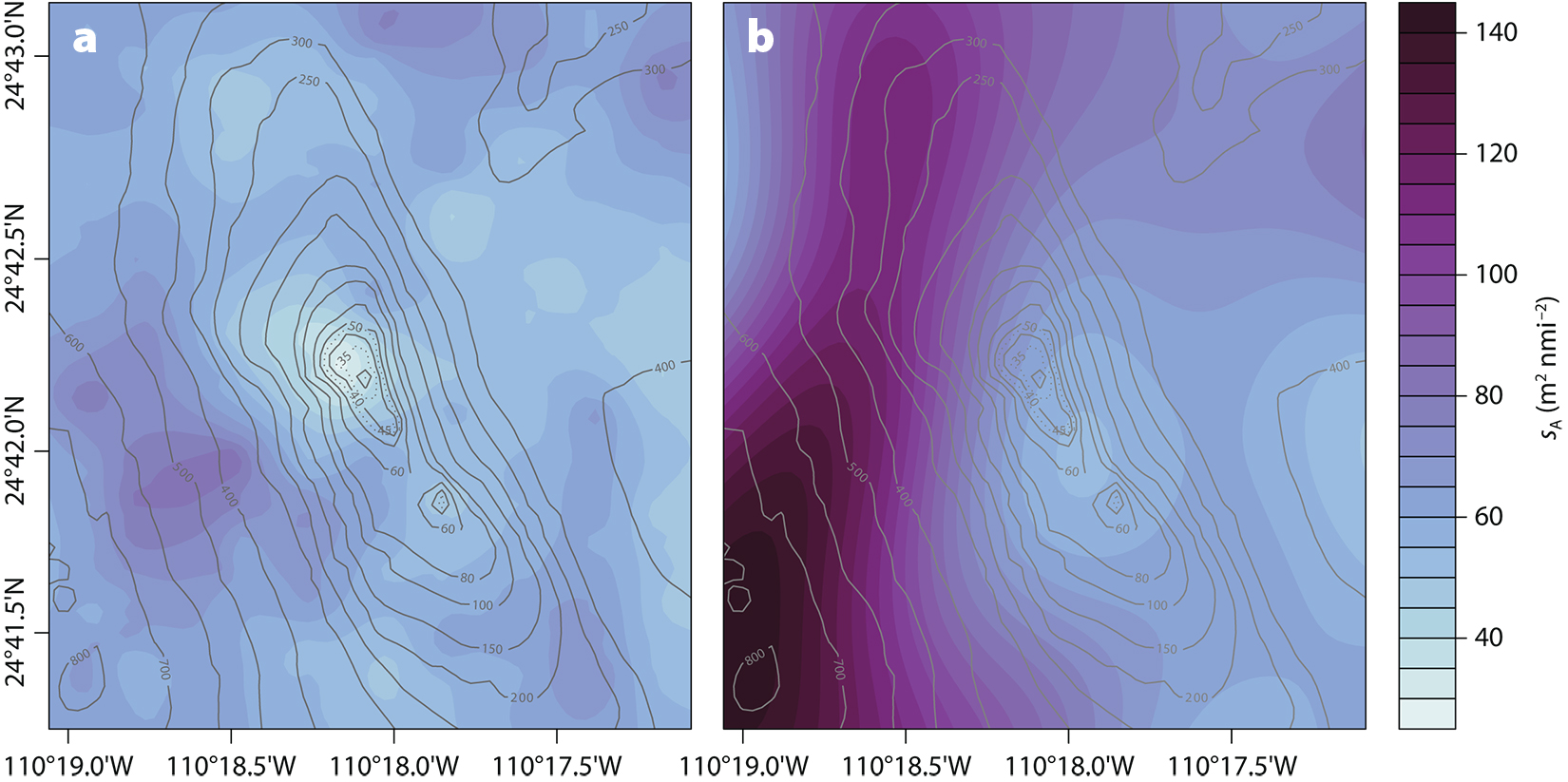
Figure 8. Comparison of interpolated zooplankton acoustic density between transects (a) 1–9 and (b) 10–16 conducted on April 21, 2018. The first pass progressed from west to east, between 12:07 and 15:15 MDT, while the second pass progressed east to west from 15:52 to 17:55 MDT. > High res figure

 

DISCUSSION

This study exemplifies the procedure for integrating acoustic, optical, and oceanographic data collection to cost-effectively survey and monitor a marine protected area. The echosounder, CTD, and camera sampling of the 2.6 nmi² EBES MPA was conducted during a ~7 hr period (excluding travel time), but with refinements, the survey could either be completed in less time or expanded to cover the entire PNZMAES. This combination of sampling methods provided data to characterize the seabed and oceanographic habitats for pelagic fishes above the seamount and to identify the predominant species present and estimate their abundances. The following sections provide a synopsis of the survey findings and suggestions for improving the efficiency and effectiveness of future surveys.

 

Bathymetry

Our bathymetric map of EBES (Figure 3) provides more detail than previously published maps, including that used to establish the MPA (Comisión Nacional de Areas Naturales Protegidas, 2006). Other maps of the area are on larger scales (e.g., Klimley and Nelson, 1984; Amador-Buenrostro et al., 2003) or their data sources and analysis methods are not described (e.g., González-Armas et al., 2002; Trasviña-Castro et al., 2003; Valle-Levinson et al., 2004). A notable difference between our bathymetry model and those of Klimley and Nelson (1984) and Amador-Buenrostro et al. (2003) is the shallowest depth (25.5 m vs 18 m, respectively). This may be due to different locations of the sampling transects, the gridding procedures and scales used, or both. To resolve this discrepancy, a multibeam echosounder should be used to construct a comprehensive map of EBES bathymetry (Kenny et al., 2003).

 

Environment

The oceanographic characteristics of EBES have not been thoroughly defined (González-Rodríguez et al., 2018), but seasonal variation is apparent (Klimley et al., 2005). During December to April, the sea surface temperature (SST) ranges from 19° to 24°C, and between May and November, it ranges from 25° to 29°C (Trasviña-Castro et al., 2003). During an El Niño event, SST tended towards the higher end of the latter range (Amador-Buenrostro et al., 2003). From July 2002 to April 2017, remotely sensed SST was lowest (~20°C) between February and March, and greatest (~30°C) during September to October (González-Rodríguez et al., 2018). Our measurements of SST during April (~22°C) are consistent with these published ranges of SST during spring.

During the transition from winter to summer conditions, the EBES area is increasingly stratified, and mixed layer depth decreases. Our measurements showed a 35 m deep mixed layer in April, compared to 20 m in June (Trasviña-Castro et al., 2003) and 19 m in May (Verdugo-Díaz et al., 2006). The salinity that we measured in the upper 100 m in April (34.8 to 35.3) is similar to that measured in the same area in June 1999 (Trasviña-Castro et al., 2003).

Our measurements of dissolved oxygen concentration may be the first published values for the EBES area. We observed a decrease in oxygen from >2.5 mL L⁻¹ above 50 m depth to <1 mL L⁻¹ at 100 m depth, and near hypoxic levels (~ 0.5 mL L⁻¹) deeper than 200 m. Throughout the Gulf of California, the depth of the oxygen minimum zone (OMZ) ranges from 100 m to 1,000 m (Hendrickx, 2001), and shoaling of the OMZ in the eastern Pacific may compress the potential habitat of marine organisms (Prince and Goodyear, 2006) compared to other areas in the world (Serrano, 2012).

 

Echo Classification

Because volume backscatter strength (S_v) varies with scatterer type (e.g., size, shape, and material properties) and number per unit volume, its dependence on acoustic wavelength or frequency is typically exploited to classify echoes. However, several methods have been used to threshold single-frequency S_v from fish versus plankton (e.g., López-Serrano et al., 2018). Our empirical –61 dB threshold at 120 kHz is very close to that used in a study of small pelagic fish (–60.7 dB; Gregg and Horne, 2009). Future surveys should include a lower frequency (e.g., 38 kHz) echosounder so the difference in volume backscatter strength measured at 120 kHz and 38 kHz may be used to better separate echoes from zooplankton and fish (Jech and Michaels, 2006). Also, for fish biomass estimations, 38 kHz may provide more precise measures compared to higher frequencies.

 

Zooplankton

In our study, backscatter from zooplankton was predominantly in the upper mixed layer (<35 m depth) and was lowest over the top of the seamount (Figure 8a). During the early afternoon, the zooplankton backscatter decreased over the top of the bank and to the northwest, suggesting that the reef fish were grazing. Later in the day, the zooplankton backscatter increased due to the diel ascent of one or more unknown species, mostly from the deepest west side of the seamount (Figure 8b). Net samples could be used to identify the zooplankton species and sizes.

 

Species Identification

The 16 reef fish species identified in the images are common in the Gulf of California (Table 2). Some of these species, for example, finescale triggerfish and yellow snapper, may be found in the upper gulf (Walker, 1960), while all of them may be present at reefs south of Isla Tiburón in the central and lower gulf (Thomson et al., 2000). All of these species have been observed at Los Islotes, located north of Espíritu Santo Archipelago (Arreola-Robles and Elorduy-Garay, 2002) and previously at EBES (Rodríguez-Romero et al., 2005). Although the fish species at EBES change seasonally (Klimley et al., 2005), year-round inhabitants may include reef fish such as scissortail damselfish, Pacific creolefish, and king angelfish (Rodríguez-Romero et al., 2005), and pelagic fish such as yellow snapper and leopard grouper (Jorgensen et al., 2016). We did not encounter pelagic fishes during our survey of EBES in April.

Scissortail damselfish was the most conspicuous and abundant species we found (Table 2). Although its aggregations have been observed at depths ranging from the reef to the sea surface (Thomson et al., 2000; Alvarez-Filip et al., 2006), we only observed damselfish schools near the seabed, where they are acoustically unresolvable, so their biomass was not estimated. Observations from the diver survey indicated schooling Pacific creolefish and finescale triggerfish close to the seafloor, but mostly swimming more than about 0.9 m above it and therefore acoustically resolvable. The acoustically unresolvable height above the seabed can be measured using multi-frequency split-beam echosounders (Demer et al., 2009).

Because reef fish may react to the presence of divers, the estimated species proportions have some unknown observational bias. Dickens et al. (2011) tried to quantify diver effects on reef fishes, and while they observed important declines in mean number of fish recorded, they concluded that underwater visual censuses are nonetheless a useful technique for estimating relative abundances. Seabed-mounted autonomous cameras may be used to mitigate any observational bias (Williams et al., 2014).

 

Fish Lengths

Landings data for EBES indicate that the total length of finescale triggerfish is generally greater than that of Pacific creolefish. The relative sizes observed in photographic images from this study confirm that finescale triggerfish were larger than Pacific creolefish at EBES in April 2018. Future surveys may include diver-​operated stereo video that, in addition to species identification, could allow estimates of fish lengths (Goetze et al., 2015; Demer et al., 2020).

 

Target Strengths

With the caveat that the echosounder was last calibrated approximately six years prior to this survey, this study produced the first published target strength measurements for in situ finescale triggerfish (mean target strength = –39.8 dB re 1 m²) and in situ Pacific creolefish (mean target strength = –34.8 dB re 1 m²). Using a common target strength versus length relationship (target strength = 20 log₁₀ (L_t (cm)) + b₂₀) and the root mean square total length values, the reduced target strength was b₂₀ = –65.2 dB for in situ Pacific creolefish and b₂₀ = –71.4 dB for in situ finescale triggerfish. These values are similar to those suggested by Foote (1987) for physoclists (–67.4 dB) and clupeoids (–71.9 dB). Note that the calibration does not affect the conversion of area backscattering coefficients to fish densities using the in situ average target strength because both sources of data were collected with the
same instrument.

 

Fish Biomass

For EBES in April 2018, our estimate of Pacific creolefish biomass is 55.7 t (95% CI = 30.3–81.2 t), which is about 40% higher than that of finescale triggerfish (38.9 t, 95% CI = 21.1–56.6 t). These estimates may be negatively biased due to the unsampled fish aggregations located close to the seabed. While fishery data for the EBES area are scarce, our biomass estimates are plausible given the 10 t yr^­–1 average catch of each species within the larger archipelago rectangle.

 

Recommendations

All of the observed reef fishes were shallower than ~200 m depth within oxygenated water. If the OMZ depth is static or shoals, future surveys of reef fishes at EBES could be constrained to the area within the 200 m isobath. Transects with smaller spacing, oriented perpendicular to the bathymetric contours, could reduce the estimation variance. More CTD casts with video cameras could be deployed along the ridge to better identify and enumerate the species of fish present and improve the characterization of their oceanographic habitat.

 

CONCLUSION

The work at EBES demonstrates that integrated acoustic, optical, and environmental sampling can be used to efficiently monitor fish populations and their essential habitats at MPAs. These technologies provide information from depths not accessible to divers. As a specific example, this study provided the most detailed bathymetric map of EBES to date, revealing a 2.5 km long and 0.8 km wide seamount with three peaks. It showed that salinity, temperature, and oxygen profiles were stratified across EBES and the mixed layer was ~35 m deep, both signaling a transitional state between winter and summer conditions. The measures of dissolved oxygen concentration at EBES, perhaps the first published values, indicate anoxic conditions below ~200 m deep. Zooplankton backscatter was mostly in the upper mixed layer and fish backscatter was in oxygenated water. Zooplankton density decreased throughout the afternoon, hypothetically due to grazing, and then increased in the evening, apparently due to diel vertical migration of one or more unknown species. Pacific creolefish and finescale triggerfish were the predominant species of schooling reef fish, with estimated biomasses of 55.7 t (95% CI = 30.3–81.2 t) and 38.9 t (95% CI = 21.1–56.6 t), respectively. These results may serve as a baseline for managers to monitor the recoveries of fish stocks at EBES (Nash and Graham, 2016) and for researchers to continue studying this
MPA ecosystem.

 

Disclaimer

This publication does not approve, recommend, or endorse any proprietary product or proprietary material mentioned herein, or which has as its purpose an intent to cause directly or indirectly the advertised product to be used or purchased because of this publication.

 

Acknowledgments

The survey and data analyses for this study were conducted during a one-week “Workshop on Acoustic-Optical Surveys,” funded by the NOAA Fisheries Advanced Sampling Technologies Program, and hosted at CICIMAR-IPN in La Paz, BCS, Mexico (April 20–27, 2018). Cesar Salinas-Zavala and Eduardo Balart (CIBNOR, SC) contributed BIP XII ship time for the survey. Lars N. Andersen (SIMRAD) and Toby Jarvis (Echoview) provided remote assistance and instruction to Mexican participants. Leonardo Figueroa-Albornoz (Kongsberg Mexico) assisted with logistics during the survey. José Manuel Borges-Souza (CICIMAR-IPN) guided the dive. The EK80 Portable used for collecting bathymetry data in April 2019 was lent by Kongsberg Maritime as part of a testing program for a low-cost scientific echosounder suitable for shallow water work across a wide range of applications. To enable his participation in this work, HV received grants from the SNI (CONACYT), and COFAA and EDI programs from IPN.

Villalobos, H., J.P. Zwolinski, C.A. Godínez-Pérez, V.E. González-Máynez, F. Manini-Ramos, M. Mayorga-Martínez, W.L. Michaels, M.S. Palacios-Higuera, U. Rubio-Rodríguez, A.N. Sarmiento-Lezcano, and D.A. Demer. 2021. A practical approach to monitoring marine protected areas: An application to El Bajo Espíritu Santo Seamount near La Paz, Mexico. Oceanography 34(3):32–43, https://doi.org/10.5670/oceanog.2021.303.

Alvarez-Filip, L., H. Reyes-Bonilla, and L.E. Calderon-Aguilera. 2006. Community structure of fishes in Cabo Pulmo reef, Gulf of California. Marine Ecology 27(3):253–262, https://doi.org/​10.1111/​j.1439-0485.2006.00108.x.

Amador-Buenrostro, A., A. Trasviña-Castro, A. Muhlia-Melo, and M.L. Argote-Espinoza. 2003. Influence of EBES seamount and Farallon basin on coastal circulation in the Gulf of California, Mexico. Geofísica Internacional 42(3):407–418.

Arreola-Robles, J.L., and J.F. Elorduy-Garay. 2002. Reef fish diversity in the region of La Paz, Baja California Sur, Mexico. Bulletin of Marine Science 70(1):1–18.

Balart, E.F., A. González-Cabello, R.C. Romero-Ponce, A. Zayas-Alvarez, M. Calderón-Parra, L. Campos-Dávila, and L.T. Findley. 2006. Length-weight relationships of cryptic reef fishes from the southwestern Gulf of California, Mexico. Journal of Applied Ichthyology 22:316–318.

Barroso-Soto, I., E. Castillo-Gallardo, C. Quiñonez-Velázquez, and R.E. Morán-Angulo. 2007. Age and growth of the finescale triggerfish, Balistes polylepis (Teleostei: Balistidae), on the coast of Mazatlán, Sinaloa, Mexico. Pacific Science 61:121–127, https://doi.org/10.1353/psc.2007.0002.

Castro, R., R. Durazo, A. Mascarenhas, C.A. Collins, and A. Trasviña. 2006. Thermohaline variability and geostrophic circulation in the southern portion of the Gulf of California. Deep Sea Research Part I 53(1):188–200, https://doi.org/10.1016/​j.dsr.2005.09.010.

Comisión Nacional de Áreas Naturales Protegidas. 2006. Estudio Previo Justificativo para el establecimiento del Área Natural Protegida “Parque Nacional Espíritu Santo.” México, D.F.

Comisión Nacional de Áreas Naturales Protegidas. 2014. Programa de Manejo. Parque Nacional exclusivamente la zona marina del Archipiélago de Espíritu Santo. SEMARNAT, México, D.F., 233 pp.

Demer, D.A., G.R. Cutter, J.S. Renfree, and J.L. Butler. 2009. A statistical-spectral method for echo classification. ICES Journal of Marine Science 66:1,081–1,090, https://doi.org/10.1093/icesjms/fsp054.

Demer, D.A. 2012. 2007 Survey of Rockfishes in the Southern California Bight Using the Collaborative Optical-Acoustic Survey Technique. Technical report, NOAA-TM-NMFS-SWFSC-498, 110 pp.

Demer, D.A., W.L. Michaels, T. Algrøy, L.N. Andersen, O. Abril-Howard, B. Binder, D. Bolser, R. Caillouet, M.D. Campbell, S. Cambronero-Solano, and others. 2020. Integrated Optic-Acoustic Studies of Reef Fish: Report of the 2018 GCFI Field Study and Workshop. NMFS-F/SPO-208, 61 pp.

De Robertis, A., and I. Higginbottom. 2007. A post-processing technique to estimate the signal-​to-​noise ratio and remove echosounder background noise. ICES Journal of Marine Science 64:1,282–1,291, https://doi.org/10.1093/icesjms/fsm112.

Dickens, L.C., C.H.R. Goatley, J.K. Tanner, and D.R. Bellwood. 2011. Quantifying relative diver effects in underwater visual censuses. PLoS ONE 6(4):e18965, https://doi.org/10.1371/journal.pone.0018965.

Emilsson, I., and M. Alatorre. 1997. Evidencias de un remolino ciclónico de mesoescala en la parte sur del Golfo de California. Pp. 173–182 in Contribuciones a la Oceanografía Física en México. M.F. Lavín, ed, Monografía 3, Unión Geofísica Mexicana.

Erisman, B., I. Mascarenas, G. Paredes, Y. Sadovy de Mitcheson, O. Aburto-Oropeza, and P. Hastings. 2010. Seasonal, annual, and long-term trends in commercial fisheries for aggregating reef fishes in the Gulf of California, Mexico. Fisheries Research 106(3):279–288, https://doi.org/10.1016/​j.fishres.2010.08.007.

Fofonoff, N.P., and R. Millard Jr. 1983. Algorithms for the computation of fundamental properties of seawater. UNESCO Technical Papers in Marine Science 44:53.

Foote, K.G. 1980. Importance of the swimbladder in acoustic scattering by fish: A comparison of gadoid and mackerel target strengths. The Journal of the Acoustical Society of America 67(6):2084, https://doi.org/​10.1121/1.384452.

Foote, K.G. 1987. Fish target strengths for use in echo integrator surveys. The Journal of the Acoustical Society of America 82(3):981, https://doi.org/​10.1121/​1.395298.

Francois, R., and G. Garrison. 1982. Sound absorption based on ocean measurements: Part II. Boric acid contribution and equation for total absorption. The Journal of the Acoustical Society of America 72(6):1879, https://doi.org/10.1121/1.388673.

Gallagher, A.J., and A.P. Klimley. 2018. The biology and conservation status of the large hammerhead shark complex: The great, scalloped, and smooth hammerheads. Reviews in Fish Biology and Fisheries 28(4):777–794, https://doi.org/10.1007/s11160-018-9530-5.

Goetze, J.S., S.D. Jupiter, T.J. Langlois, S.K. Wilson, E.S. Harvey, T. Bond, and W. Naisilisili. 2015. Diver operated video most accurately detects the impacts of fishing within periodically harvested closures. Journal of Experimental Marine Biology and Ecology 462:74–82, https://doi.org/10.1016/​j.jembe.2014.10.004.

González-Armas, R., R. Palomares-García, and R. De Silva-Dávila. 2002. Copepod and macrozooplankton distribution associated to El Bajo Espíritu Santo Seamount. Pp. 183–193 in Contribution to the Study of East Pacific Crustaceans. M.E. Hendrickx, ed, Instituto de Ciencias del Mar y Limnología, UNAM, México.

González-Rodríguez, E., A. Trasviña-Castro, and A. Ramos-Rodríguez. 2018. El Bajo de Espíritu Santo; punto caliente de abundancia biológica afuera de Bahía de La Paz. CICIMAR Oceánides 33(1):13–24, https://doi.org/10.37543/oceanides.v33i1.224.

Gregg, M.C., and J.K. Horne. 2009. Turbulence, acoustic backscatter, and pelagic nekton in Monterey Bay. Journal of Physical Oceanography 39(5):1,097–1,114, https://doi.org/​10.1175/2008JPO4033.1.

Hendrickx, M.E. 2001. Occurrence of a continental slope decapod crustacean community along the edge of the minimum oxygen zone in the southeastern Gulf of California, Mexico. Belgian Journal of Zoology 131(suppl. 2):95–109.

Hernández-Ortiz, D.X. 2013. Evaluación de la efectividad del Parque Nacional Zona Marina del Archipiélago Espíritu Santo como herramienta de conservación y generación de beneficios socioeconómico. BSc Thesis, Universidad Autónoma de Baja California Sur, La Paz, BCS, México.

Hewitt, R., and D. Demer. 1991. Krill abundance. Nature 353:310, https://doi.org/10.1038/353310b0.

Jech, J.M., and W.L. Michaels. 2006. A multifrequency method to classify and evaluate fisheries acoustics data. Canadian Journal of Fisheries and Aquatic Sciences 63(10):2,225–2,235, https://doi.org/​10.1139/F06-126.

Jorgensen, S.J., A.P. Klimley, A. Muhlia-Melo, and S.G. Morgan. 2016. Seasonal changes in fish assemblage structure at a shallow seamount in the Gulf of California. PeerJ 4:e2357, https://doi.org/​10.7717/peerj.2357.

Kenny, A.J., I. Cato, M. Desprez, G. Fader, R. Schüttenhelm, and J. Side. 2003. An overview of seabed-mapping technologies in the context of marine habitat classification. ICES Journal of Marine Science 60(2):411–418, https://doi.org/​10.1016/​S1054-3139(03)00006-7.

Klimley, A.P., and D.R. Nelson. 1984. Diel movement patterns of the scalloped hammerhead shark (Sphyrna lewini) in relation to El Bajo Espíritu Santo: A refuging central-position social system. Behavioral Ecology and Sociobiology 15(1):45–54, https://doi.org/10.1007/BF00310214.

Klimley, A.P., and S. Butler. 1988. Immigration and emigration of a pelagic fish assemblage to seamounts in the Gulf of California related to water mass movements using satellite imagery. Marine Ecology Progress Series 49(1):11– 20, https://doi.org/​10.3354/​meps049011.

Klimley, A.P., J.E. Richert, and S.J. Jorgensen. 2005. The home of blue water fish: Rather than singly inhabiting the trackless ocean, pelagic fish species travel together in groups, which migrate between hidden, productive oases. American Scientist 93(1):42–49.

Ladroit, Y., P.C. Escobar-Flores, A.C.G. Schimel, and R.L. O’Driscoll. 2020. ESP3: An open-source software for the quantitative processing of hydro-acoustic data. SoftwareX 12(2020):100581, https://doi.org/10.1016/j.softx.2020.100581.

López-Serrano, A., H. Villalobos, and M.O. Nevárez-Martínez. 2018. A probabilistic procedure for estimating an optimal echo-integration threshold using the Expectation-Maximisation algorithm. Aquatic Living Resources 31:12, https://doi.org/10.1051/alr/2017048.

Michaels, W.L., B. Binder, K. Boswell, L.M. Chérubin, D.A. Demer, T. Jarvis, F.R. Knudsen, C. Lang, J.E. Paramo, P.J. Sullivan, and others. 2019. Best Practices for Implementing Acoustic Technologies to Improve Reef Fish Ecosystem Surveys: Report from the 2017 GCFI Acoustics Workshop. NOAA Technical Memo NMFS-F/SPO-192, 161 pp., https://spo.nmfs.noaa.gov/sites/default/files/​TM192.pdf.

Nash, K.L., and N.A. Graham. 2016. Ecological indicators for coral reef fisheries management. Fish and Fisheries 17(4):1,029–1,054, https://doi.org/10.1111/faf.12157.

Ortega-Rubio, A., I. González-López, I. March-Mifsut, E.I. Bustamante-Moreno, M.Á. Palmeros-Rodríguez, N. Bojórquez-Galeana, A. Suárez, and B. Bermúdez-Almada. 2019. Parque Nacional Zona Marina del Archipiélago Espíritu Santo: Primer Área Natural Protegida de México con el Certificado Lista Verde de UICN. Áreas Naturales Protegidas Scripta 5(1):43–68.

Pérez-Jiménez, J.C. 2014. Historical records reveal potential extirpation of four hammerhead sharks (Sphyrna spp.) in Mexican Pacific waters. Reviews in Fish Biology and Fisheries 24(2):671–683, https://doi.org/10.1007/s11160-014-9353-y.

Petitgas, P. 1993. Geostatistics for fish stock assessments: A review and an acoustic application. ICES Journal of Marine Science 50(3):285–298, https://doi.org/10.1006/jmsc.1993.1031.

Petitgas, P., and A. Prampart. 1995. EVA Estimation VAriance: logiciel de géostatistique pour l’analyse structurale et les calculs de variance. ORSTOM.

Prince, E.D., and C.P. Goodyear. 2006. Hypoxia-based habitat compression of tropical pelagic fishes. Fisheries Oceanography 15(6):451–464, https://doi.org/​10.1111/j.1365-2419.2005.00393.x.

R Core Team. 2020. R: A Language and Environment for Statistical Computing. R Foundation for Statistical Computing, Vienna, Austria.

Ribeiro, P.J. Jr., and P.J. Diggle. 2018. geoR: Analysis of Geostatistical Data. R package version 1.7-5.2.1.

Robles, J.M., and S.G. Marinone. 1987. Seasonal and interannual thermohaline variability in the Guaymas Basin of the Gulf of California. Continental Shelf Research 7(7):715–733, https://doi.org/​10.1016/​0278-4343(87)90013-6.

Rodríguez-Romero, J., A.F. Muhlia-Melo, F. Galván-Magaña, F.J. Gutiérrez-Sánchez, and V. Gracia-López. 2005. Fish assemblages around Espíritu Santo island and Espíritu Santo Seamount in the lower Gulf of California, Mexico. Bulletin of Marine Science 77(1):33–50.

Ryan, T.E., R.A. Downie, R.J. Kloser, and G. Keith. 2015. Reducing bias due to noise and attenuation in open-ocean echo integration data. ICES Journal of Marine Science 72(8):2,482–2,493, https://doi.org/​10.1093/​icesjms/fsv121.

Sala, E., O. Aburto-Oropeza, G. Paredes, and G. Thompson. 2003. Spawning aggregations and reproductive behavior of reef fishes in the Gulf of California. Bulletin of Marine Science 72(1):103–121.

Saldaña-Ruiz, L.E., O. Sosa-Nishizaki, and D. Cartamil. 2017. Historical reconstruction of Gulf of California shark fishery landings and species composition, 1939–2014, in a data-poor fishery context. Fisheries Research 195:116–129, https://doi.org/10.1016/​j.fishres.2017.07.011.

Schlitzer, R. 2015. Ocean Data View User’s Guide. Alfred Wegener Institute, Bremerhaven, Germany, 150 pp.

Secretaría de Medio Ambiente y Recursos Naturales. 2007. Decreto por el que se declara área natural protegida, con la categoría de Parque Nacional exclusivamente la zona marina del Archipiélago de Espíritu Santo, ubicado en el Golfo de California, frente a las costas del Municipio de La Paz, Baja California Sur. Diario Oficial de la Federación, 10 de mayo de 2007. Primera sección. México.

Serrano, D. 2012. La zona del mínimo de oxígeno en el Pacífico mexicano. Pp. 105–119 in Biodiversidad y comunidades del talud continental del Pacífico mexicano. P. Zamorano, M.E. Hendrickx, and M. Caso, eds, Secretaría del Medio Ambiente y Recursos Naturales, Instituto Nacional de Ecología.

Simmonds, E.J., and D.N. MacLennan. 2005. Fisheries Acoustics: Theory and Practice. Blackwell, Oxford, 456 pp.

Thomson, D.A., L.T. Findley, and A.N. Kerstitch. 2000. Reef Fishes of the Sea of Cortez: The Rocky-Shore Fishes of the Gulf of California, Revised edition. University of Texas Press, Austin, Texas, 407 pp.

Torres-Orozco, E. 1993. Análisis volumétrico de las masas de agua del Golfo de California. MSc Thesis, Centro de Investigación Científica y Educación Superior de Ensenada (CICESE), Ensenada, B.C., México.

Trasviña-Castro, A., G. Gutierrez de Velasco, A. Valle-Levinson, R. González-Armas, A. Muhlia, and M. Cosio. 2003. Hydrographic observations of the flow in the vicinity of a shallow seamount top in the Gulf of California. Estuarine, Coastal and Shelf Science 57(1-2):149–162, https://doi.org/10.1016/S0272-7714(02)00338-4.

Valle-Levinson, A., A. Trasviña-Castro, G. Gutiérrez de Velasco, and R. González-Armas. 2004. Diurnal vertical motions over a seamount of the southern Gulf of California. Journal of Marine Systems 50(1–2):61–77.

Verdugo-Díaz, G., R. Cervantes-Duarte, and M.O. Albañez-Lucero. 2006. Variación estacional de la productividad primaria estimada por fluorescencia natural en El Bajo Espíritu Santo, BCS, México. Naturaleza y Desarrollo 4(2):35–40.

Walker, B.W. 1960. The distribution and affinities of the marine fish fauna of the Gulf of California. Systematic Zoology 9(3/4):123–133, https://doi.org/​10.2307/2411961.

Williams, K., A. De Robertis, Z. Berkowitz, C. Rooper, R. Towler. 2014. An underwater stereo-camera trap. Methods in Oceanography 11:1–12, https://doi.org/​10.1016/j.mio.2015.01.003.

This is an open access article made available under the terms of the Creative Commons Attribution 4.0 International License (https://creativecommons.org/licenses/by/4.0/), which permits use, sharing, adaptation, distribution, and reproduction in any medium or format as long as users cite the materials appropriately, provide a link to the Creative Commons license, and indicate the changes that were made to the original content. Images, animations, videos, or other third-party material used in articles are included in the Creative Commons license unless indicated otherwise in a credit line to the material. If the material is not included in the article’s Creative Commons license, users will need to obtain permission directly from the license holder to reproduce the material.