This interdisciplinary work demonstrates the viability of coupling ocean models with in situ robotic sampling in a dynamic coastal region as a means to increase model skill and prediction. Model-driven exploration closes the sample-assimilate-​predict-direct loop within a virtuous cycle to refine prediction for a range of applications in a region characterized by harsh conditions, high variability, and diverse physical forcings, including bathymetry and coastal topography. By exploring the feasibility of coupling high-resolution autonomous underwater vehicle (AUV) sampling and data assimilation with a geostatistical model in a continuous loop, we aim to provide a new approach to understanding coastal dynamics and processes, while using modest computational resources. The novelty of this effort is threefold: the demonstration of coupling models with AUV sampling, the importance of targeted sampling, and the impact of loop closure toward model prediction.

Introduction

The marine areas extending from the coastline to the continental slope and encompassing the continental shelf, known collectively as the coastal ocean, constitute one of the most dynamic and complex regions of the ocean. These areas are characterized by high variability and intricate topographies and coastline geometries. They are forced by a wide range of physical and biogeochemical processes that occur across diverse spatial and temporal scales. They are among the most productive and economically significant areas of the world ocean, benefiting from terrestrial inputs via river discharges and nutrient renewal driven by upwelling processes. As a result, and in part, coastal areas concentrate a great proportion of human activities, including leisure, fisheries, offshore aquaculture, and renewable energy exploitation. The coastal ocean mediates interactions between deep-ocean processes and coastal environments, influencing how large-scale phenomena—such as climate-driven changes or extreme weather events—affect the coastal population. It also governs, for example, how anthropogenic influences originating on land are redistributed and affect marine ecosystems (Greene and Delaney, 2025).

Interactions among physical, chemical, and biological processes in the coastal ocean can amplify or mitigate the impacts of extreme events, including storms, flooding, and pollution. Furthermore, the coastal ocean serves as a key interface where large-scale oceanic and atmospheric changes manifest their consequences for coastal ecosystems. Accurately forecasting the state of the coastal ocean is therefore essential not only for safeguarding environmental and economic interests but also for enhancing resilience to climate variability, natural hazards, and anthropogenic stressors.

Ocean models have become essential tools for predicting ocean state, and they underpin a wide range of societal applications, from climate forecasting to pollution monitoring and resource management. However, these models are inherently imperfect representations of complex reality. Data assimilation techniques, where observational data are integrated to update models, play a critical role in correcting or adjusting model errors and improving their forecasting capabilities. Yet, the success of data assimilation depends heavily on the availability, quality, and relevance of observations.

Satellite remote sensing provides extensive spatial coverage but is generally limited to surface observations and constrained by atmospheric conditions. In situ observations from ships, moorings, or drifting platforms, although spatially sparse and logistically demanding, complement satellite data by providing higher spatial or temporal resolution and access to subsurface processes, adding a critical three-dimensional component to the observing system. Recent technological advances have enabled the use of autonomous underwater vehicles (AUVs) and other robotic platforms, offering flexible, mobile, and increasingly autonomous means of sampling ocean properties with high spatiotemporal resolution and low logistic footprints (Das et al., 2012, 2015; Graham et al., 2012; Fossum et al. 2018).

However, even with these new tools, efficiently collecting data for modeling at optimal spatial and temporal scales remains a complex challenge. AUVs are constrained not only by endurance and communication bandwidth but also by speed (typically on the order of 1–2 ms^–1), which is comparable to ambient current velocities and thus limits synopticity. This limitation is even more pronounced for gliders, as they operate at lower effective speeds. Operational risks that further restrict deployment include vessel traffic, fishing activity, strong currents, and complex bathymetry. In addition, the ocean itself remains highly dynamic, with key processes often evolving faster than traditional ship-based sampling strategies can capture. This opens the door to adaptive sampling strategies, where observation efforts are guided by model outputs and uncertainty estimates to maximize the relevance of collected data. Adaptive sampling (Zhang and Sukhatme, 2007; Singh et al., 2009; Fossum et al., 2019a) represents a fundamental shift: instead of executing pre-planned missions, autonomous vehicles dynamically prioritize areas for observation. Our approach combines model predictions with adaptive sampling using propelled AUVs. Lermusiaux (2007), Ford et al. (2022), and Wihsgott et al. (2026) explore such a concept, with Lermusiaux in simulation only. While Ford et al. (2022) focus a single glider on chlorophyll as a driver, and Wihsgott et al. (2026) multiple gliders on chlorophyll, temperature, and oxygen, we target temperature exclusively. The novelty of our work is in demonstrating the applicability of controlling the AUV’s trajectory using onboard computation and articulating the importance of the larger sample-​assimilate-​predict-​direct loop. Our setup is also simpler as we employ the Copernicus Marine Service (CMEMS) Nucleus for European Modelling of the Ocean (NEMO) numerical model, which is used to initiate the stochastic model, the primary model we use in our work. This is supplemented with practical ways to reduce operational costs using small boat operations and multiple in-house designed AUVs with our mature technology suite for command/control.

Model forecasts identify where spatial uncertainty is highest or where new observations are expected to have the greatest impact in reducing forecast errors. Vehicles are then directed to sample these areas, and their data are in turn assimilated back into the models, as a virtuous cycle. Data assimilation from these high uncertainty regions is then incorporated into the model so that new predictions benefit from improved in situ data. Such an approach promises to significantly enhance the skill of ocean forecasts, especially in the complex coastal environment where processes occur over a wide range of scales.

Our work has three significant results. First, it demonstrates the importance of coupling ocean models with high-resolution AUV sampling. Second, it highlights the importance of targeted adaptive sampling based on model uncertainty. Third, it demonstrates the importance of assimilation in predicting and closing the sample-​assimilate-​predict-​direct loop (Figure 1). Additionally, sampling resolution with AUVs vastly outweighs that of the data obtained from traditional ship-based approaches. Using multiple AUVs sampling simultaneously, as we do here, also makes a dent in spatial as well as temporal coverage of dynamic environments at relatively moderate costs. Finally, AUVs can provide near-real-time data, allowing for their rapid re-tasking and potential placement in evolving spatially separated regions.

 

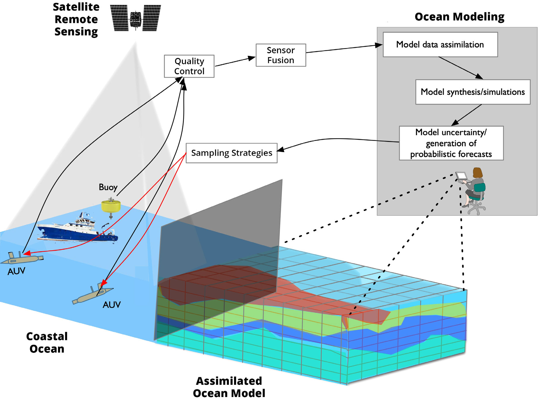
FIGURE 1. The work described here was conducted within the framework of FRESNEL (Field expeRiment for modEling, aSsimilatioN and adaptivE sampling. It demonstrates the value of integrating ocean models with adaptive robotic vehicles in the coastal ocean to increase model skill and prediction within a tight control loop. > High res figure

 

This manuscript is organized as follows. We first introduce the problem we are tackling, providing a motivation for the sample-​assimilate-​predict-​direct loop. Next, we provide the environmental context and the challenge of modeling and operating robotic vehicles in a dynamic coastal region. Our Methods section then highlights the details of the forecasting, assimilation, sampling, and operational strategies that lie at the core of this paper. We next highlight the results of our experiment, followed by a discussion and analysis of these results. We wrap up with conclusions and propose future work.

 

Study Area

In this study, we address the challenge of loop closure by implementing and evaluating a complete data cycle, from model prediction, to uncertainty generation, to adaptive sampling, to data assimilation. The work was conducted within the framework of FRESNEL (Field expeRiments for modEling, aSsimilatioN and adaptivE sampLing), specifically designed to explore and test model-driven robotic exploration strategies.

The study was conducted off central Portugal, focusing on the region influenced by the Nazaré Canyon (39.2°–39.9°N; Figure 2) during fall 2024. While the experiment considered the measurable impact of model-driven robotic sampling on the biogeochemistry of the canyon region, this manuscript focuses on the implications of closing the sample-​assimilate-​predict-​direct loop closure.

 

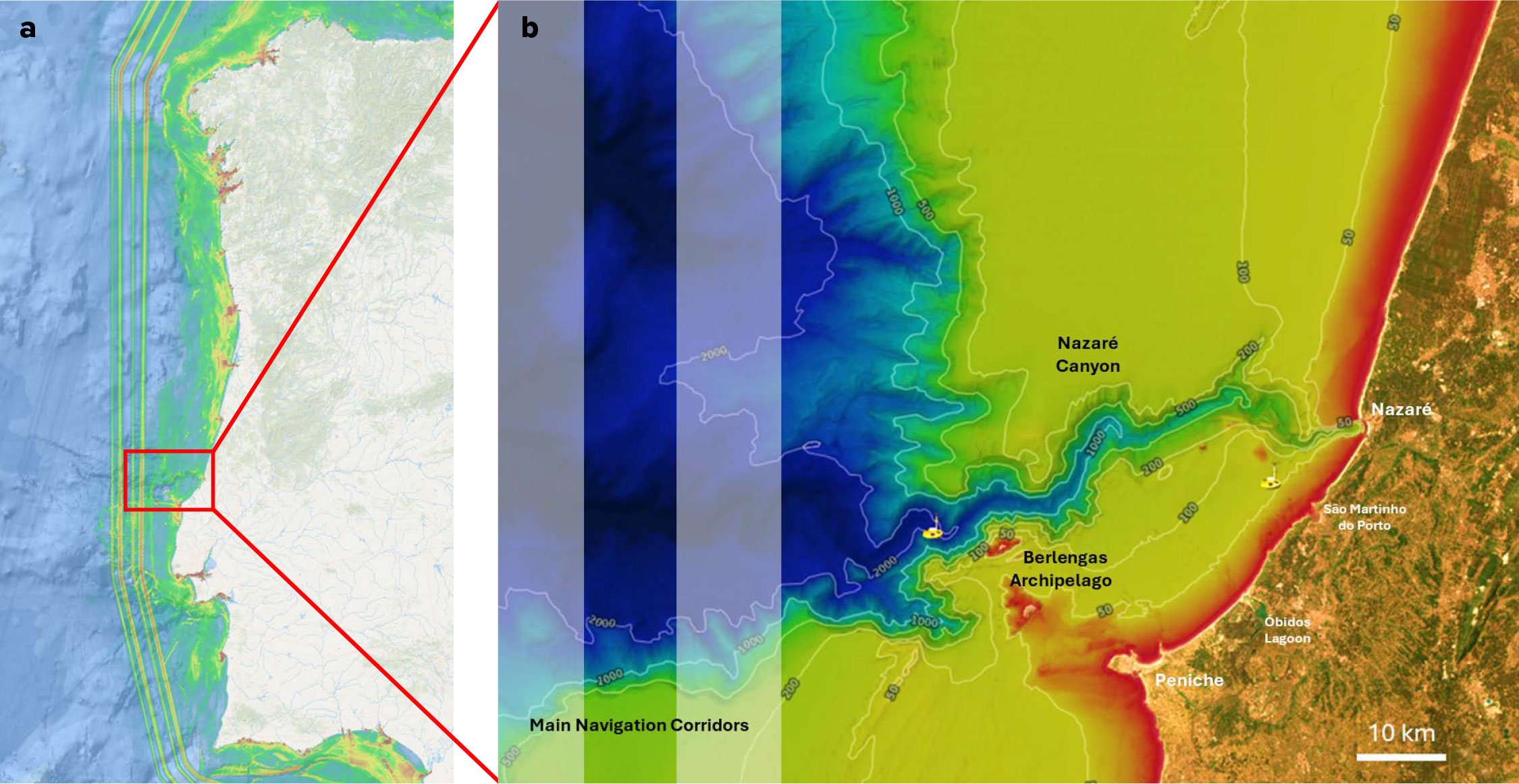
FIGURE 2. (a) Map of Portugal’s west coast with the study area highlighted with a red rectangle. (b) The bathymetry of the FRESNEL study area includes the Nazaré Canyon-Berlengas area and its environment. The white bands indicate commercial shipping lanes. The two buoys drawn on the map are part of a coastal observing system. The Nazaré Canyon is a significant feature of this area and a driver for the biogeophysics of the domain (Tyler et al., 2009), along with other prominent features. > High res figure

 

Implementing such a closed-loop system in a dynamic coastal environment presents substantial challenges. These include the need for spatial high-resolution numerical models capable of rapidly generating uncertainty predictions, robust algorithms for exploration under a range of constraints, reliable communication links for mission updates, and assimilation frameworks that integrate heterogeneous real-time data streams. Furthermore, marine operations face logistical risks and communication limitations, such as intermittent connectivity, unpredictable weather, and vessel traffic, that further constrain the execution of robotic missions.

The Nazaré area features pronounced topographic contrasts: the transition from the wide Estremadura Plateau to the narrower northern shelf, the long and narrow Nazaré submarine canyon that incises the shelf and extends more than 200 km offshore, and the Berlengas archipelago, a UNESCO Biosphere Reserve with high ecological value. These features contribute to enhanced biological productivity and biodiversity and strongly modulate physical and biogeochemical processes in the region.

Freshwater inputs from major rivers, such as the Tagus, have only a limited direct impact on the area. In contrast, smaller rivers and the Óbidos lagoon, located south of Nazaré, can episodically deliver low-salinity, nutrient-rich plumes to the shelf. Circulation is driven by seasonal wind forcing linked with the Azores High, with persistent upwelling-favorable northerly winds in summer and frequent downwelling episodes in winter under southerly winds. The interplay between canyon topography, shelf circulation, and atmospheric forcing generates complex mesoscale dynamics, intensified tidal currents, and internal wave activity that promote strong vertical mixing and cross-shelf exchanges (Quaresma et al., 2007; I. Martins et al., 2010).

The combination of sharp bathymetric gradients, variable forcing, and rich physical-biogeochemical interactions makes the Nazaré Canyon region an ideal natural laboratory for testing sampling strategies and evaluating how model-based uncertainty projections can guide sampling and assimilation to improve ocean model predictive skill.

 

Methods

Our methodology is based on implementing a closed-loop data cycle to improve predictions from a coastal ocean model via robotic adaptive sampling and data assimilation. The approach consists of three fundamental steps, executed iteratively daily:

Model Forecast and Uncertainty Projection. An ocean model provides a daily step forecast 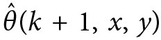 of a target oceanic variable θ, along with an associated uncertainty field 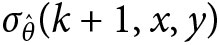, where k represents the current day and (x, y) denote the geographical coordinates. These outputs are organized into discrete spatial maps,  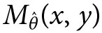and 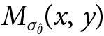, representing the predicted state and its uncertainty, respectively, over a predefined grid covering the study area.

Targeted Sampling. We define areas of larger uncertainty predictions as areas of higher “reward” to bias where the AUVs sample. Using the uncertainty map as input, the targeted sampling algorithm determines the set of trajectories for N AUVs for the next operational cycle, typically the following day. The goal is to maximize the accumulated uncertainty sampled along the vehicle trajectories.

Data Collection and Assimilation. Throughout the operational cycle, each AUV collects measurements of the target variable θ along its assigned path. After mission completion, the collected measurements are assimilated into the model using an appropriate data assimilation scheme. This updated model state serves as the new initial condition for the next forecasting cycle, closing the loop.

While previous efforts have concentrated on a form of embedded and automated decision-making for AUV-based adaptive sampling (McGann et al., 2008; Ryan et al., 2010; Garcia-Olaya et al., 2012; Rajan and Py, 2012), the trajectories in this work are generated offline, with adaptation focused on deployment based on . Here, loop closure refers to the sample-​assimilate-​predict-​direct process.
 

Model Forecast, Uncertainty Projection, and Data Assimilation

Sampling strategies rely on timely information about the spatial variability of ocean properties. Conventional numerical ocean circulation models, based on the fluid dynamics, such as CMEMS NEMO (EU Copernicus Marine Service [CMEMS] Information Marine Data Store [MDS], 2024a), Regional Ocean Modeling System (ROMS; Shchepetkin and McWilliams, 2005), and Hybrid Coordinate Ocean Model (HYCOM; Wallcraft et al., 2009), for example, are widely used by the scientific community for operational forecasting and research. These models provide physically consistent simulations of ocean state variables (e.g., temperature, salinity, currents) and underpin applications ranging from climate prediction to coastal management. However, numerical ocean models are computationally intensive, and their runtime makes them impractical for use with high spatial resolution and in near-real-time mission planning (Agarwal et al., 2021). While assimilation-prediction cycles such as the one we propose could, in principle, be implemented within such models, it would require either substantially larger computational resources or longer execution times.

As a practical alternative, we use geostatistical simulation (i.e., direct sequential simulation; Soares, 2001) as a computationally efficient surrogate for short-term spatial predictions of ocean variables together with estimates of spatial uncertainty (Deutsch and Journel, 1992). This approach captures the essential spatio­temporal variability of local ocean dynamics, based on a prior numerical ocean model solution, at a fraction of the computational cost of numerical models, while remaining flexible enough to rapidly assimilate new in situ observations (Duarte et al., 2025). However, with these types of surrogate models, we are not explicitly considering the full physics of the system, and the quality of the predictions directly depends on the accuracy of the numerical model and the prediction time length. If the numerical model is unable to capture the true nature of the system, the geostatistical predictions will likely be inaccurate.

Our methodology relies on ensembles of geostatistical realizations, each representing a state of an ocean variable field conditioned a priori by the deterministic CMEMS NEMO model (Madec et al., 1997, 2015; EU Copernicus Marine Service [CMEMS] Information Marine Data Store [MDS], 2024a) using the Iberian Biscay Irish domain. In doing so we use a variogram model describing the temporal dependency between days over a 14-day period. Realizations are generated via stochastic sequential simulation: the grid is visited along a random path and, at each node, the local Kriging mean and variance are computed from the covariance/variogram model and the available conditioning data, from which a value is drawn from the corresponding conditional distribution. By computing the pointwise standard deviation across the ensemble, we obtain spatial uncertainty maps that highlight regions where predictions are more variable and therefore potentially a target for robotic sampling. These maps then, serve as the basis for identifying areas where new measurements are expected to maximize the reduction of forecast error.

Beyond uncertainty prediction, the statistical approach incorporates AUV data through sequential assimilation, refining forecasts for subsequent cycles. Data collected on a given day is used to update the ocean variable forecast for the following day by combining prior predictions with new measurements. The geostatistical simulation grid, in this case, includes two temporal layers: the first contains the AUV measurements at their spatial locations, and the second corresponds to the new prediction step. With AUV sampling denser than the model horizontal grid resolution (approximately 0.0035°, corresponding to about 300–400 m at the study latitude), measurements within the same grid cell are averaged as a form of arithmetic upscaling (Duarte et al., 2025). To incorporate spatial and temporal variability, we apply sequential simulation with local means (Soares, 2001),¹ where each simulated value is drawn from its conditional distribution, accounting for both prior simulated values and local mean models. Doing so enables consistent updating of the variable field while integrating both AUV observations and a priori information. The ensemble of realizations thus provides an updated ocean forecast and a quantitative measure of uncertainty.

The spatial and temporal continuity of the variable field is simultaneously characterized by variogram models fitted to long-term numerical ocean model data from CMEMS NEMO. For each depth layer of the numerical model where the AUV navigation is defined, geostatistical simulations are performed independently using a moving temporal window of the previous 14 days as conditioning data. This window length was selected through comparison with the numerical model’s short-term evolution under similar seasonal conditions, striking a balance between forecast stability and computational cost. Spatial propagation occurs only horizontally within each depth level, while vertical consistency is implicitly maintained through the depth-specific variogram structures derived from the 3D numerical model (see Figure 3 of Duarte et al., 2025). This provides both a forecast of the ocean variables being simulated and a quantitative assessment of the prediction uncertainty. By updating the forecasts with new in situ measurements through sequential assimilation, the method progressively refines the variable field while maintaining consistency with prior model dynamics. The resulting forecast and uncertainty maps then form the input for the targeted sampling algorithm, guiding the allocation of AUV trajectories toward regions of greatest expected information gain. Duarte et al. (2025) provide a complete description of the methodology and implementation.

---

¹ Defined by Kriging estimates and variances, which are conditioned to existing direct measurements and a spatial covariance matrix (Cressie, 1993).

---

The Sampling Algorithm

Our adaptive sampling problem involves the design of vehicle trajectories that maximize information gain (Eidsvik et al., 2015; Fossum et al., 2018) extracted from the uncertainty map provided by the model, while satisfying operational AUV constraints. Each day, the model provides both a forecast field and its associated uncertainty distribution, which together define the reward landscape for the trajectory planner. The task is to generate, for each vehicle, a tour that accumulates the highest possible uncertainty values. The tour is traveled at a prescribed AUV speed while the duration is bounded above by the assimilation period. The starting and ending points are selected to simplify logistics for launch and recovery.

Although the underlying numerical CMEMS NEMO model is fully three-dimensional and the statistical solution also provides predictions across multiple depth layers, in this work, the sampling algorithm operates on a two-dimensional (2D) horizontal field derived from the uncertainty structure of the statistical solution. This field is obtained by averaging the horizontal depth slices of uncertainty between the surface and 40 m depth, a depth interval chosen to represent the upper mixed layer in the Nazaré study region. Within this layer, turbulent mixing typically maintains relatively weak vertical gradients, and most of the temperature variability relevant for mission planning is concentrated near the surface and the upper thermocline. Averaging across this depth range, therefore, yields a stable and physically meaningful representation of the uncertainty field.

While the trajectory planning itself is carried out in two dimensions, the yo-yo motion executed by the AUVs along each transect naturally restores vertical sampling capability, compensating for the 2D approximation and enabling the acquisition of high vertical resolution profiles at all visited locations. This strategy also aligns with the dominant physical and biogeochemical processes occurring within the mixed layer, where air-sea interactions, nutrient entrainment, and local thermal structure exert primary control on short-term dynamics (Behrenfeld and Boss, 2014; Mahadevan, 2016).

The tour is formulated as a graph theoretic problem. The spatial uncertainty map is first pre-processed to remove obstacles and smoothed to highlight large-scale features. Candidate waypoints are then identified from the map and used to build a weighted graph, where nodes carry a reward proportional to their uncertainty value and edges represent travel costs. The trajectory planning task is posed as a multi-vehicle, multi-depot tour routing problem where routes must balance the rewards obtained from visiting nodes with associated costs of traveling between them (Vidal et al., 2013; Toth and Vigo, 2014). By solving this graph traversal problem, the algorithm returns a set of near-optimal trajectories that prioritize regions of greatest uncertainty while enforcing an effective travel budget (endurance) and an obstacle-masked admissible area (safety) (Bernacchi et al., 2025). This is illustrated by the boundaries in the uncertainty field shown in the zoomed area of Figure 4b.

Operations and Data Collection

The in situ data collection process involved three upper water-​column light autonomous underwater vehicles (LAUVs; XP2, XP3, and XP5)² that performed targeted sampling missions with durations of up to 60 hours over the Nazaré Canyon region, with all vehicles sampling the upper 100 m of the water column. These vehicles were designed and developed in-house at the University of Porto (Sousa et al., 2012) and are equipped with a range of sensors, including a CTD (Figure 3a), along with Wi-Fi and Iridium satellite communications. The CTDs mounted on the AUVs were cross calibrated to ensure consistency. In addition to the hardware involved, we used an extensive suite of mature mission planning and command/control tools whose discussion is outside the scope of this paper and can be found in Dias et al. (2005), R. Martins and Sousa (2010), and Pinto et al. (2013).

 

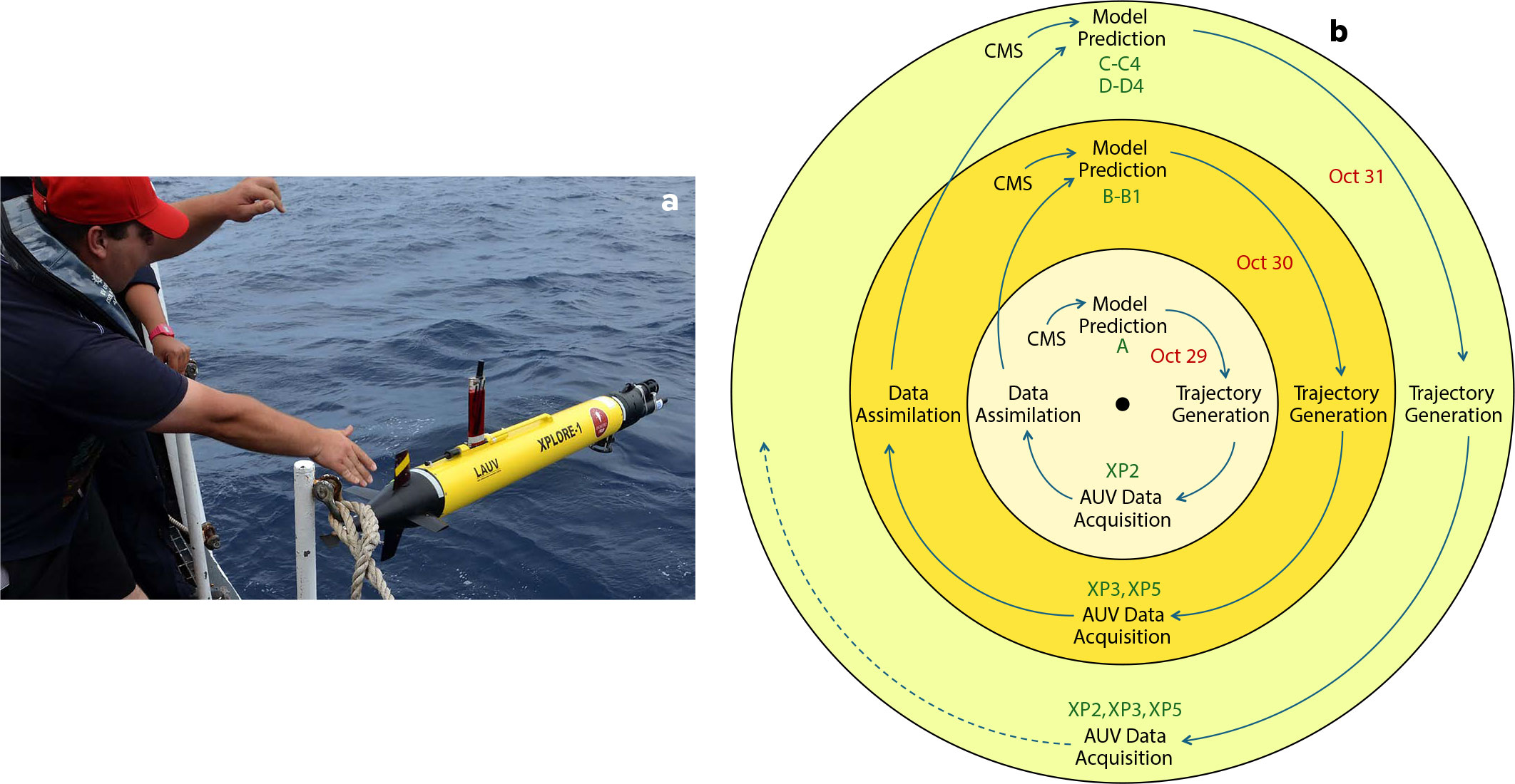
FIGURE 3. (a) Multiple light autonomous underwater vehicles (LAUVs), such as the one in this photo, were used in FRESNEL. This low-cost platform designed at the University of Porto has proven to be robust, is easily integrated with a number of oceanographic sensors, and comes with sizable open source command/control software. See the supplemental video for LAUV XP5 recovery at sea. (b) Three-day sequence (October 29–31, 2024) of the sample-assimilate-predict-direct loop in the FRESNEL experiment. Each cycle integrated statistical model predictions using the EU Copernicus Marine Service Information (CMEMS) Copernicus Marine Service Nucleus for European Modelling of the Ocean (NEMO) model as a prior, targeted sampling, AUV data acquisition, and subsequent assimilation for the following day’s prediction. > High res figure

 

The experiment had a small human and support vessel footprint, demonstrating significant cost reduction in comparison to traditional ship-based methods while measuring at higher spatial and temporal resolution. Operations were conducted continuously by pairs of operators working six-hour shifts based in Porto as well as locally in Nazaré—small boat use was limited to the launch and recovery of AUVs, which operated unattended.

Challenging meteorological and ocean conditions constrained the number of consecutive iterations of the sample-​assimilate-​predict-​direct loop to a three-day sequence of experiments (October 29–31, 2024; Figure 3b). Also for simplicity and clarity, we focused on a single variable: temperature measurements. As a consequence, this work is univariate in showing the impact of assimilated model-driven exploration. We believe that the experimental results presented in this paper are general enough to apply to other critical physical oceanographic variables, which would be modeled similarly. Therefore, the analysis presented here ultimately aims to quantify the impact of assimilating AUV-acquired temperature data on the predictive performance of the statistical model and to assess the operational feasibility of the data cycle approach in a coastal setting.

Each experimental day followed a structured cycle that involved (1) the generation of a statistical model forecast and its associated uncertainty field using the prior CMEMS NEMO model data available up to the previous day (Sotillo et al., 2021), (2) the execution of the target sampling algorithm to plan the next day mission, (3) in situ data collection by AUVs following the algorithmically determined tours, (4) and, finally, assimilation of data from the tour into the model.

---

² We will refer to these specific vehicles across the three-day period based on the diversity and specificity of their operating environments and measurements.

---

A Multi-Scenario Framework

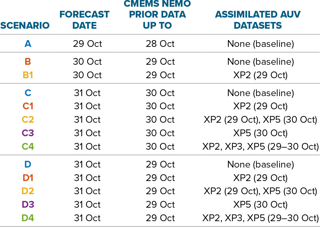
Given the logistical and weather-related challenges encountered, a number of scenarios contribute to the final solution set. The scenarios are labeled A through D (and their corresponding assimilation variants) in Table 1, which provides a compact, color-​coded overview of all configurations (used in Figure 6), including statistical forecast dates, prior CMEMS NEMO fields, and the specific AUV datasets assimilated at each stage.

 

TABLE 1. Summary of scenarios and assimilation configurations. The color codes are referred to in Figure 6 to disambiguate root mean square error plots. > High res table

 

On October 29, 2024, the statistical model produced the initial forecast solution (A), which was used to plan the mission executed by XP2 (Figure 3b). The resulting data were assimilated offline to produce an updated statistical model solution (B1) for October 30. Although operational real-time assimilation was initially planned, logistical constraints prevented its implementation; consequently, all assimilations were performed offline after AUV mission completion. The targeted sampling algorithm, therefore, relied on statistical forecasts without assimilation (B), using pre-existing data as input for daily mission planning. This limitation is not expected to have significantly affected the experimental outcomes, as the operational area was compact and the predicted variability field remained consistent between consecutive days.³

For October 31, multiple assimilation configurations were tested to quantify how the information collected on previous days could influence short-term predictive skill. Measurements from XP3 and XP5 on October 30 were assimilated offline to generate scenarios C1–C4, complementing the non-assimilated reference case C. These cases progressively integrate different subsets of AUV observations, ranging from XP2-only data (C1) to the full multi-vehicle dataset from October 29 to 30 (C4).

A parallel set of scenarios (D and D1–D4) was generated to evaluate the sensitivity of the statistical model to the choice of prior CMEMS NEMO fields. The D-series uses CMEMS NEMO data available only up to October 29, thus representing a less favorable initial state, and applies the same assimilation configurations as in the C-series. This dual-series approach enables a controlled comparison of how data assimilation interacts with differences in model initialization. Model performance was evaluated by comparing predicted and observed temperature data along the AUV trajectories using root mean square error (RMSE) as the performance metric for October 31.

FRESNEL is part of a larger concept for multi-domain sensing, observation, and exploration that couples ocean models, autonomous robotics, artificial intelligence, and machine learning with a small satellite constellation. Our end goal is to democratize ocean model prediction using low-cost operations integrated with open-source software to enable spatio-temporal data assimilation from mobile or immobile robots across space, aerial, surface, and underwater domains (Rajan et al., 2021).

---

³ In future implementations, on-board or near-real-time assimilation would need to be considered to fully exploit the framework’s adaptive potential.

---

 

Experimental Results

Figure 4a summarizes environmental conditions observed during the three-day experimental window considered in this study. The background fields correspond to the Level 3 sea surface temperature (SST) product (EU Copernicus Marine Service (CMEMS) Information Marine Data Store (MDS), 2024b). The operational area covers approximately 100 km² south of Nazaré Canyon. While all missions focused on temperature variability predicted by the model, on October 31, XP2 was deployed for a cross-shore transect of approximately 13 km to sample an internal wave hotspot; in this study, it serves as an independent ground-truth dataset. These observations are used as a reference for evaluating the forecast cases C1–C4 and D1–D4. See online supplementary material for more information regarding AUV paths.

During the experimentation, the coastal ocean was influenced by a late-season upwelling-relaxation cycle. At the beginning of the sequence (October 29), the SST field revealed the characteristic signature of coastal upwelling, with colder water masses extending offshore due to wind-driven Ekman transport that brings subsurface, nutrient-rich waters to the surface. In the following days, the weakening of upwelling-favorable winds led to a relaxation phase, during which warmer offshore waters gradually advanced toward the coast. This transition is reflected in the SST maps by an overall warming trend in the nearshore region, particularly evident on November 1 (Figure 4a).

 

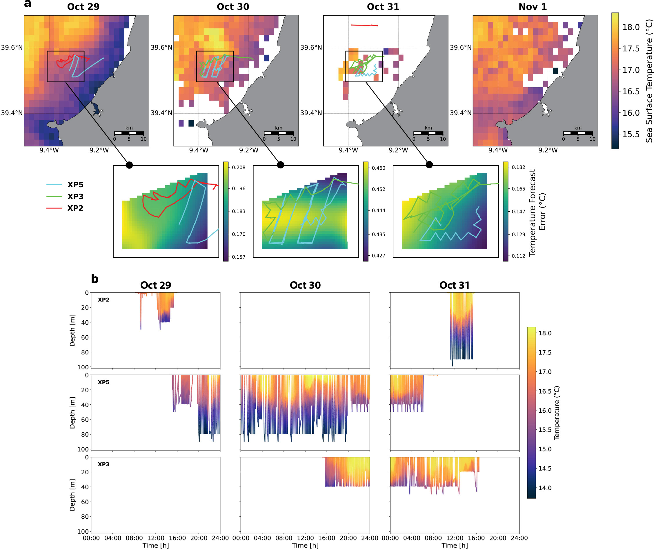
FIGURE 4. (a) L3 sea surface temperature (SST) remote sensing product CMEMS Marine Data Store (MDS), and AUV trajectories during the FRESNEL experiment, October 29–31, overlaid with the statistical-model uncertainty field (i.e., temperature forecast error) for the duration of the experiment in October. (b) Time-depth temperature evolution observed by AUVs in the same period. > High res figure

 

It is important to note that the SST imagery is partially affected by cloud coverage, which limits the availability and accuracy of satellite-derived temperature data. Despite these limitations, the SST patterns clearly capture the dominant mesoscale features and coastal processes driving the observed variability during the experiment. The pronounced temperature gradients associated with the upwelling front generated well-defined spatial and temporal variability, making the impact of targeted in situ observations on predictive model skill visible.

Figure 4b shows the vertical temperature distribution measured by the AUVs between October 29 and 31. The panels illustrate the temporal and vertical structure of the coastal water column throughout the three-day period, and they highlight the complexity of logistics in multi-vehicle operations, where scheduling, resources, and environmental constraints together determine the actual temporal coverage of the vehicles.

XP2 operated on October 29 and 31, XP5 on October 29, 30, and 31, and XP3 on October 30 and 31. The temperature fields reveal a thermocline and a progressive warming of the surface layer down to approximately 40 m depth, with temperatures ranging from ~14°C in deeper layers to ~18°C near the surface, reaching their maximum on the afternoon of October 30 during XP5’s mission.

In Figure 5, four scatter plots compare the measurements acquired in situ on October 31 against the corresponding geostatistical predictions derived under each scenario. They focus on the most contrasted scenarios: the baseline cases without assimilation (C and D) and those incorporating the full set of AUV observations from previous days (C4 and D4). The observations include all available data collected by the missions on that day (see Figure 4a,b). Colors indicate the depth layers associated with the vertical discretization used in the CMEMS NEMO model, which defines the vertical structure of the statistical model. This comparison illustrates the statistical model’s ability to reproduce the observed temperatures at each measurement point accurately, contrasting the non-assimilated cases (C and D) with the partially and fully assimilated (C1–C4 and D1–D4).

 

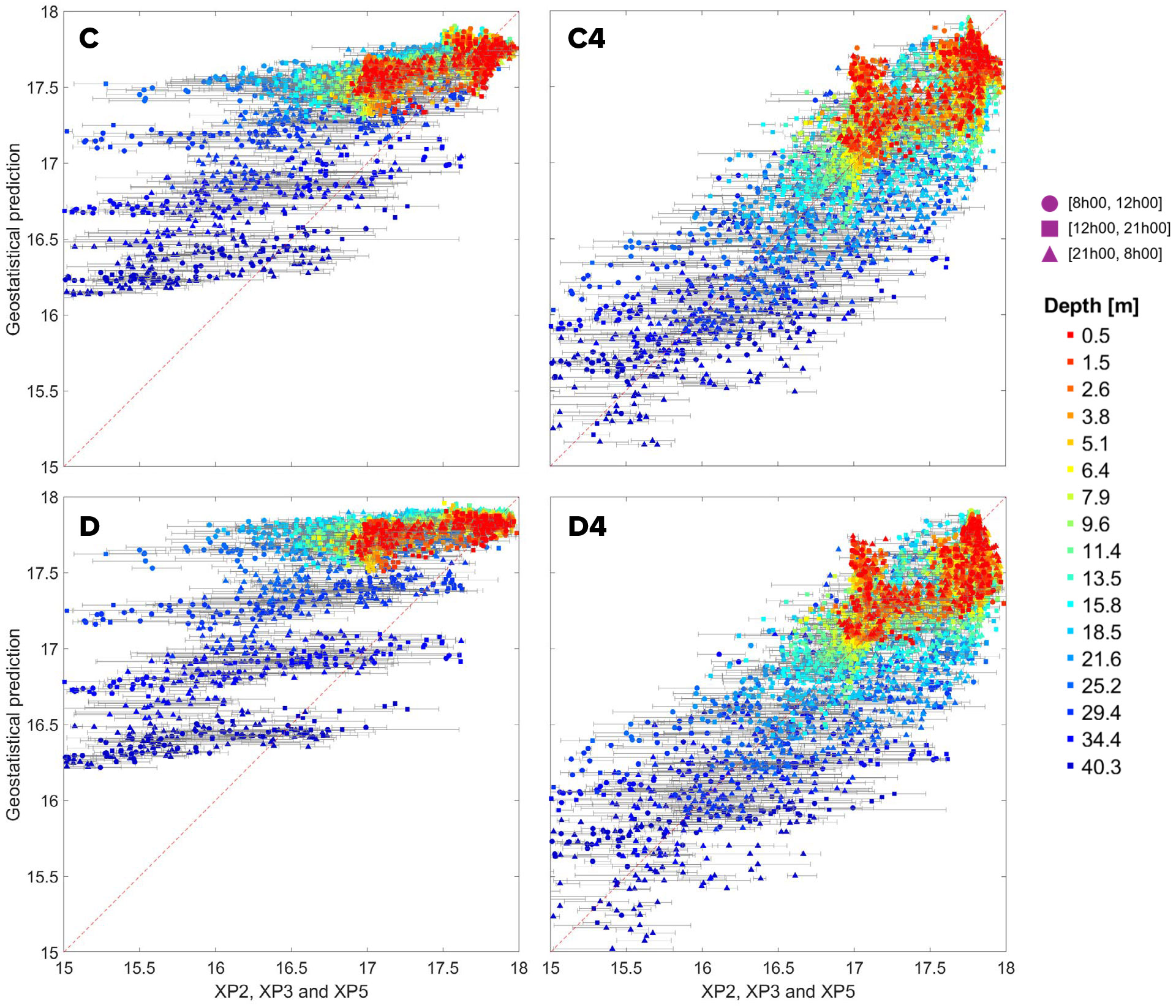
FIGURE 5. Comparison between in situ AUV temperature (°C) observations (October 31) and model temperature (°C) scenarios C, C4, D, and D4. Shallower layers are shown in warmer colors (red to yellow), while deeper layers (>30 m) are progressively represented in cooler shades (green to blue). The dashed red line provides a reference for correlation. > High res figure

 

In the baseline scenarios without assimilation (C and D), the plots exhibit a wide spread of points around the reference line, indicating substantial discrepancies between the model predictions and the observed AUV measurements. These deviations are particularly evident in XP3 and XP5 data, where temperatures around 20–30 m depth tend to be overestimated by almost 1°C (Figure 6b,c). This dispersion reflects the model’s limited ability to accurately reproduce the vertical thermal structure when it relies solely on CMEMS NEMO data without incorporating in situ information.

In contrast, the fully assimilated scenarios (C4 and D4) show a much tighter clustering of points around the reference, especially within the studied upper layers, where the previous AUV missions provide dense and temporally relevant observations. This reduction in spread suggests a clear improvement in predictive accuracy, indicating that the assimilation of targeted measurements effectively constrains the thermal structure and captures ongoing physical transitions in the water column. See the online supplementary material for a detailed comparison of SST fields across the CMEMS NEMO model products from C to C4 and from D to D4.

Figure 6 presents the RMSE between the statistical model forecasts and the in situ temperature observations collected by the AUVs. These figures cover all experimental configurations examined in this study. Figure 6a corresponds to the initial phase of the experiments on October 29 and 30. Scenario A represents the baseline statistical forecast based on CMEMS NEMO data. B and B1 scenarios correspond to forecasts for October 30 without and with the assimilation of in situ observations during the previous day (see Table 1). RMSE values in scenario A range from approximately 0.48°C near the surface to 1.33°C at 40 m, with a mean RMSE of about 0.74°C. The errors increase with depth, indicating reduced model skill in reproducing the subsurface thermal structure. The non-assimilated B scenario remains similar to A in the upper layers but diverges below 20 m. Assimilation in scenario B1 consistently improves predictions across the water column compared to the non-assimilated B scenario with RMSE values between 0.31°C and 0.55°C and an average of 0.39°C representing an overall reduction of nearly 50% relative to B. This improvement is most pronounced in the 5–20 m layers, coinciding with the strongest vertical temperature gradients and the region most densely sampled by the AUVs.

 

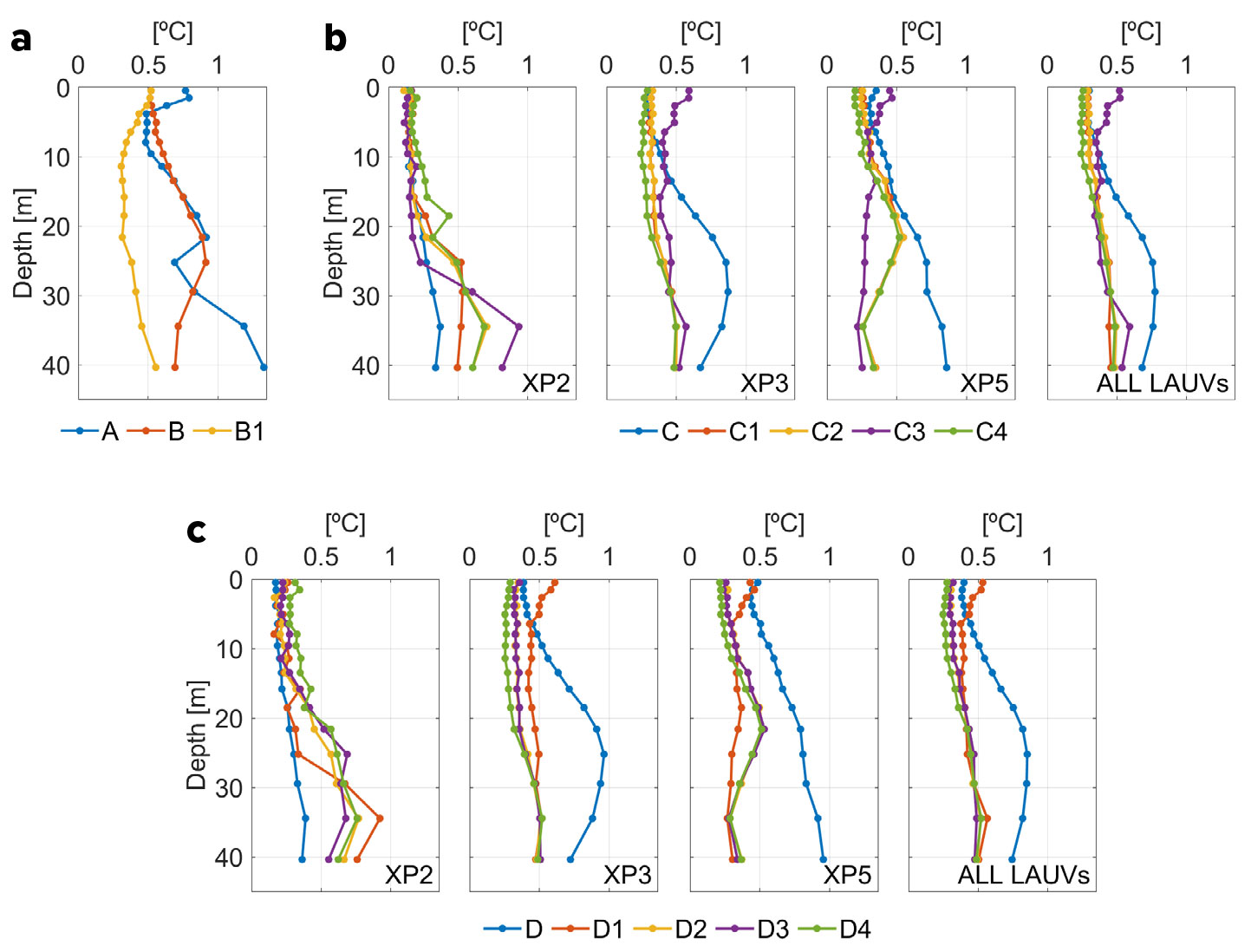
FIGURE 6. (a) Root mean square error (RMSE) in °C between model forecasts and in situ AUV temperature observations for October 29–30. Scenario A corresponds to the baseline statistical forecast generated based on CMEMS NEMO data up to October 29. Scenarios B and B1 represent forecasts for October 30 without and with, respectively, the assimilation of AUV observations collected by light autonomous underwater vehicle (LAUV) XP2. (b) RMSE, between the statistical model forecasts and in situ AUV temperature measurements for October 31, for scenarios C and C1–C4. These forecasts were initialized using Copernicus Marine Service Nucleus for European Modelling of the Ocean (CMEMS NEMO) data available up to October 30, and the assimilation steps progressively incorporate AUV observations collected on previous days. Results are shown for each vehicle and for the combined dataset (“All LAUVs”). (c) Same as (b), but for scenarios D and D1–D4, in which forecasts for October 31 were initialized using CMEMS NEMO data available only up to October 29. Assimilation configurations D1–D4 mirror those of the C-series but start from this less favorable prior state. Results are again presented per vehicle and for the aggregated dataset. > High res figure

 

The results for October 31, summarized in Figure 6, correspond to the phase of the experiment in which multiple assimilation scenarios were tested. The C-series used CMEMS NEMO data up to October 30, whereas the D-series uses CMEMS NEMO up to October 29, representing a less favorable statistical initial state. In both cases, the assimilation scenarios (C1–C4 and D1–D4) correspond to the incorporation of AUV data collected during previous days (see Table 1).

A consistent reduction in statistical forecast error is observed across most vehicles and assimilation stages. In the C-series, the average RMSE across all AUVs decreases from approximately 0.40°C in C to 0.31°C in C4, while in the D-series, the mean RMSE drops from 0.55°C in D to 0.40°C in D4 (see Table 1). These improvements correspond to an average error reduction of 25%–30%, demonstrating that the assimilation of targeted observations can compensate for differences in the initial state and improve predictive accuracy.

For XP3 and XP5, which performed targeted sampling in the same area where previous assimilation data were collected, RMSE values show a consistent reduction. In contrast, XP2, which on October 31 performed a cross-shore transect outside the main target region, exhibits a weaker response to assimilation. The implications of this behavior and its relevance for evaluating the predictive robustness of the framework are examined in the next section. Vertically, RMSE profiles show similar behavior in both experiment sets: errors tend to increase gradually below 25–30 m, where model uncertainty and unresolved variability are higher. However, this gradient weakens considerably in the fully assimilated cases (C4 and D4), particularly in the upper 30 m, where the assimilation of prior AUV data significantly improves the representation of the temperature structure and short-term thermal evolution probably associated with the upwelling-relaxation transition.

 

Discussion

Assessing the impact of targeted AUV observations on short-term ocean forecasts requires evaluating both model-data agreement and how assimilation effects vary across regions and dynamical oceanographic regimes. Although assimilation generally improves model skill, vehicle-specific results highlight differences linked to sampling patterns and regional dynamics.

Figure 6b,c presents the RMSE predictions compared with in situ data under the different assimilation scenarios (C, C4, D, and D4) for October 31. The results are shown as a function of depth and vehicle, allowing a direct comparison with and without data assimilation. For XP3 and XP5, a clear and consistent trend is observed: the assimilation scenarios (C4 and D4) improve the model prediction skill, with RMSE decreasing across all depths, indicating that the assimilation procedure effectively constrains the local dynamics represented in the statistical model. Although small differences are present between C4 and D4, they are not statistically significant and confirm that assimilation results are robust with respect to initial configuration differences.

The situation for XP2 was different, however. The assimilation scenarios (C4 and D4) lead to higher prediction errors compared with the non-assimilation runs (C and D). This counterintuitive result reflects a spatial mismatch: on October 31, XP2 operated north of Nazaré Canyon, while assimilated data from the previous days (October 29 and 30) were collected south of it. Nazaré Canyon marks a transition zone between distinct oceanographic regimes, where circulation patterns are strongly influenced by the canyon’s complex topography and the interaction between shelf and slope processes. Inside the canyon, residual currents are generally aligned along the canyon axis as a result of strong topographical forcing, and this alignment extends well above the canyon edges (~150 m depth), implying substantial disturbance of the predominant north-south circulation parallel to the general trend of the shelf and slope (Relvas et al., 2007; Tyler et al., 2009; Guerreiro et al., 2014). This topographic forcing not only alters circulation but also serves as a conduit for transporting organic matter and sediment from the shelf to the deep sea. The divergence in physical regimes at the canyon likely supports distinct biological assemblages, or “hotspots” of productivity that would be misrepresented by a model that fails to capture these subgrid dynamics (de Stigter et al., 2007; Cunha et al., 2011).

CMEMS NEMO fields (Figure 7) provide a broader context, comparing temperature distributions in northern and southern regions of the study area during the days preceding and during the experiment. Before October 26, although mean temperatures differ between the two regions, their variability is consistent, indicating that the system was evolving coherently across the canyon, with systematically colder waters (by about 1°C) in the northern region. After October 26, the temperature evolution in the two regions diverges, with the CMEMS NEMO model showing relatively warmer conditions in the north compared to the south. This divergence coincides with the onset of the upwelling-​relaxation transition and highlights a shift toward slightly distinct dynamical regimes on either side of the canyon. This transition can explain why assimilation of southern data, collected under a single dynamical regime, fails to improve and, in fact, degrades forecasts. An alternative explanation for the divergence of the results, which may also act in combination with previously explained factors, concerns the choice of covariance length scales. In our configuration, the estimated variogram range is approximately 70 km in the horizontal, with a temporal correlation scale of about one season. The variogram parameters are estimated using data from the entire domain of interest, which can be interpreted as capturing an “average” space-time behavior. As a consequence, this single, domain-​wide covariance model cannot represent local heterogeneity, such as differences between the southern and northern sectors of the Nazaré Canyon region. Therefore, local over- and/or under-estimation of the variogram range may lead to overly broad or overly localized background corrections, which can in turn increase the RMSE in the assimilative experiments (C4 and D4) relative to the corresponding baseline runs (C and D) without assimilation.

 

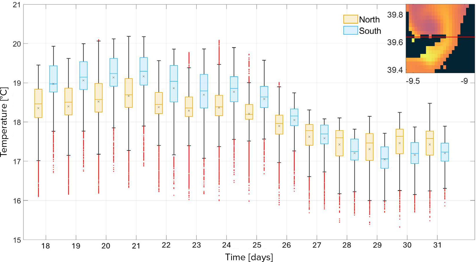
FIGURE 7. Temperature distributions from CMEMS NEMO for the northern and southern regions of the study area between October 18 and 31. The division between regions follows the line boundary shown in the inset map, top right. Only grid points shallower than 200 m were retained to avoid including the canyon interface. Boxplots show the spatial distribution of CMEMS NEMO temperature within each region, capturing both the median and the spread of variability. > High res figure

 

This spatial mismatch underscores the need for trajectory-​planning strategies that maximize class separation between distinct dynamical regimes, as proposed by Fossum et al. (2019b) using hierarchical clustering methods. Such approaches, based on criteria including variance reduction, mutual information, or entropy, could help identify routes that better discriminate between competing oceanographic states and mitigate situations where assimilation may propagate misleading information if relying solely on uncertainty fields.

Another highlight of this experiment was in showing the variability within the model grid, which provided additional insight into the subgrid-scale structure of the observed field. Figure 8 depicts the interquartile distance (IQD) of measurements recorded by the AUVs within the three-dimensional discretization of the statistical model. Each grid cell represents the maximum spatial resolution available in the model, while the IQD quantifies the local variability of in situ measurements acquired as the vehicles navigated through each cell.

 

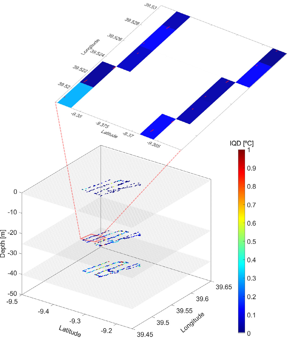
FIGURE 8. Trajectory of LAUV XP5, during the October 30 mission in the Nazaré Canyon region. The color shading represents the interquartile range (IQD) of temperature values recorded within each model grid cell, illustrating the horizontal resolution of the statistical model. Results are shown for three representative depth layers: near-surface, 20 m, and 40 m, capturing distinct vertical regimes. Higher IQD values indicate regions of higher thermal variability within the model grid. Close-up view of the 20 m layer reveals fine-scale fluctuations occurring inside single grid elements, illustrating that the AUVs are capturing subgrid-scale structure that the model does not resolve. > High res figure

 

This figure illustrates how robotic platforms can capture significant variability at scales smaller than the model resolution, revealing the existence of fine-scale gradients, in some locations greater than 1°C, as processes that are also unresolved by the model. Although the statistical model provides smoothed, grid-​averaged predictions of ocean properties, AUV measurements highlight fluctuations that occur within individual cells, indicating the presence of subgrid-scale dynamics. Unresolved variability is a known source of error in data assimilation systems; numerical forecasts and statistical surrogates inevitably smooth or filter variability below grid scale, so observations that resolve submesoscale or turbulent features will often disagree locally with grid-​averaged model fields (Oke and Sakov, 2008; Janjić et al., 2018). These considerations underscore that high-resolution observations from AUVs should not be interpreted solely through coarse model fields. Instead, subgrid variability itself provides valuable information about local forecast uncertainty and should be explicitly accounted for when assimilating observations into coarser-​resolution predictive systems.

Across all missions, the AUVs sampled each grid cell with median values ranging from 9 to 14 measurements per cell and mean values between 19 and 26. These statistics indicate a relatively uniform and dense sampling pattern, sufficient to characterize the local variability of the water column at the subgrid level. The maximum number of samples per grid cell reached several thousand available to communicate and geolocate, though these values are biased by vehicle behavior near the surface.

Despite these localized biases, the overall sampling density achieved by the AUVs provides a detailed depiction of fine-scale ocean variability. The IQD distributions reveal higher variability near the thermocline (30–40 m), where vertical gradients are strongest, while in some instances increased variability could also appear near the surface, potentially corresponding to small-scale frontal zones or localized mixing events. Because AUVs sample continuously along their trajectories, they resolve spatial and temporal scales that often fall between CTD stations in traditional ship-based surveys, thereby capturing subgrid processes that remain unresolved in numerical models.

This subgrid variability is not observational noise; it provides valuable insight into local uncertainty and environmental heterogeneity. For example, quantifying this variability is essential for biological oceanography, as many marine organisms—from zooplankton to fish larvae—aggregate in micro-fronts or thermal patches that are often smaller than model resolution. Understanding this “noise” helps distinguish biological aggregations from physical turbulence (Visser and Stips, 2002). Incorporating both the variability (such as IQD) and the spatial sampling density into data assimilation frameworks enhances the model’s ability to represent uncertainty at the subgrid scale and improve the realism of short-term forecasts.

This field study provides invaluable lessons in operational procedures, refinement of adaptive sampling and algorithms, and risk minimization for operating in an area with dense ship traffic and fishing nets. Our AUVs were occasionally affected by strong vertical currents that may have resulted from the impact of internal waves that are common in the area and that were observed with the help of remote-sensing imagery during the experiment.

Finally, the results achieved with this deployment provided additional insights and the motivation to further advance the state of the art in refining the sample-​assimilate-​predict-​direct cycle with the goal of improving the skill of oceanographic models. Furthermore, dense grids of sampled oceanographic data have the potential to fuel developments that target existing gaps in modeling skill when different levels of spatial and temporal resolution are considered (Balaji et al. 2022).

 

Conclusions

This effort demonstrates the usefulness of overall integration to close the sample-​assimilate-​predict-​direct cycle to improve oceanographic model skill by leveraging observations from robotic platforms. Figure 6 shows clear indications of an increase in predictive skill when high-resolution data from AUVs are assimilated in a geostatistical model. By choosing such a modeling approach, this effort offers a window into the rapid process of assimilating and predicting, the primary goal of FRESNEL, and doing so with minimal operational support. The accuracy of the predictions of the geostatistical model increased after several cycles, while overall prediction errors decreased as noted. These results provide a foundation for continuous ocean prediction when obtaining high-resolution in situ data as conceptualized in the METEOR (A Mobile (Portable) ocEan roboTic ObsErvatORy) framework (Rajan et al., 2021).

A confluence of external factors reduced the observation period from the planned three weeks to three days, primarily due to weather, platform availability, and personnel constraints. Future work will extend the observation period to validate and expand upon these promising results.

Other challenges that remain to be addressed include near-real-time assimilation and continuous model prediction, especially to capture dynamic coastal events. While we are still lacking the desired statistical significance of a long series of consecutive cycles, our future work will target optimization of the parameters used for deeper integration of the algorithms used in the cycle. For instance, we hope to investigate the selection of representative depths for the application of the sampling algorithm used to find the horizontal projection of the AUV paths (Bernacchi et al., 2025). Another potential outcome to be investigated is the use of higher-resolution numerical models and longer prediction horizons, considering computational trade-offs. In doing so, we would also like to demonstrate the viability of portable low (computational) cost models running in the cloud, which can be initialized for any region rapidly to demonstrate the loop-closure we set out to validate.

Along these lines, an additional research direction involves encapsulating a model surrogate embedded within the control system of one or more AUVs to capture coastal dynamism at fine scales (Frolov et al., 2009; Fossum et al., 2019b), while complementing an increase in the assessment of shore-based model skill.

 

Acknowledgments

This work was carried out with the support of the US Office of Naval Research (ONR), contract N00014-22-1-2796. We are grateful to Tom Drake (Code 32) for his support. RM and JBS acknowledge the support of Fundação para a Ciência e a Tecnologia (FCT) for its financial support to LAETA via the project UID/50022/2025. LA and AD gratefully acknowledge the support of CER-ENA (UID/04028/2025). MC and CR thank UID Centro de Estudos do Ambiente e Mar (CESAM) + LA/P/0094/2020 for support. AD is funded by the Fundação para a Ciência e a Tecnologia (FCT, Portuguese Foundation for Science and Technology) through project PRT/BD/154661/2023. The work was also partially supported by JUNO—Robotic Exploration of Atlantic Waters project—Refa 2021/0008 from FLAD, by the DiverSea project (grant # 101082004) supported by the European Commission and the TRAINEE project (2024.07606.IACDC) supported by FCT. Finally, we would like to thank the two anonymous reviewers whose comments and critique have contributed substantially to strengthening this manuscript.

Mendes, R., A.F. Duarte, L. Azevedo, L. Bernacchi, J.B. de Sousa, J. Pereira, B. Gabriel, J. Bogas, M. Cunha, C.F. Rodrigues, A. Subramaniam, F. Esteves, and K. Rajan. 2026. Toward ocean model-driven robotic exploration. Oceanography 39(2):34–47, https://doi.org/10.5670/oceanog.2026.e209.

- LAUV XP5 recovery at sea (video)

- Additional analysis and figures (pdf)

1. Agarwal, N., D. Kondrashov, P. Dueben, E. Ryzhov, and P. Berloff. 2021. A comparison of data-driven approaches to build low-dimensional ocean models. Journal of Advances in Modeling Earth Systems 13(9):e2021MS002537, https://doi.org/​10.1029/2021MS002537.
2. Balaji, V., F. Couvreux, J. Deshayes, J. Gautrais, F. Hourdin, and C. Rio. 2022. Are general circulation models obsolete? Proceedings of the National Academy of Sciences of the United States of America 119(47):e2202075119, https://doi.org/​10.1073/pnas.2202075119.
3. Behrenfeld, M.J., and E.S. Boss. 2014. Resurrecting the ecological underpinnings of ocean plankton blooms. Annual Review of Marine Science 6(1):167–194, https://doi.org/​10.1146/annurev-marine-052913-021325.
4. Bernacchi, L., A.F. Duarte, R. Mendes, L. Azevedo, and J.B. de Sousa. 2025. Closing the data loop: Real-world AUVs adaptive sampling for improved ocean model predictions. Pp. 1–8 in 2025 Symposium on Maritime Informatics and Robotics (MARIS). June 26–27, 2025, Syros, Greece, IEEE, https://doi.org/10.1109/MARIS64137.2025.11139688.
5. Cressie, N.A.C. 1993. Statistics for Spatial Data. Revised Edition, Wiley, New York, 928 pp., https://doi.org/10.1002/9781119115151.
6. Cunha, M.R., G.L. Paterson, T. Amaro, S. Blackbird, H.C. de Stigter, C. Ferreira, A. Glover, A. Hilario, K. Kiriakoulakis, L. Neal, and others. 2011. Biodiversity of macrofaunal assemblages from three Portuguese submarine canyons (NE Atlantic). Deep Sea Research Part II 58(23–24):2,433–2,447, https://doi.org/10.1016/j.dsr2.​2011.04.007.
7. Das, J., F. Py, T. Maughan, M. Messie, T. O’Reilly, J. Ryan, G.S. Sukhatme, and K. Rajan. 2012. Coordinated sampling of dynamic oceanographic features with AUVs and drifters. International Journal of Robotics Research 31(5), https://doi.org/​10.1177/0278364912440736.
8. Das, J., F. Py, J.B. Harvey, J.P. Ryan, A. Gellene, R. Graham, D.A. Caron, K. Rajan, and G.S. Sukhatme. 2015. Data-driven robotic sampling for marine ecosystem monitoring. International Journal of Robotics Research 34:(12):1,435–1,452, https://doi.org/​10.1177/0278364915587723.
9. de Stigter, H.C., W. Boer, P.A. de Jesus Mendes, C.C. Jesus, L. Thomsen, G.D. van den Bergh, and T.C. van Weering. 2007. Recent sediment transport and deposition in the Nazaré Canyon, Portuguese continental margin. Marine Geology 246(2–4):144–164, https://doi.org/10.1016/j.margeo.2007.04.011.
10. Deutsch, C.V., and A.G. Journel. 1992. GSLIB: Geostatistical Software Library and User’s Guide. Oxford University Press, New York, first edition, 340 pp.
11. Dias, P.S., S.L. Fraga, R.M. Gomes, G.M. Goncalves, F.L. Pereira, J. Pinto, and J.B. Sousa. 2005. NEPTUS - A framework to support multiple vehicle operation. Pp. 963–968 in Europe Oceans 2005. June 20–23, 2005, Paris, France, IEEE, https://doi.org/10.1109/OCEANSE.2005.1513187.
12. Duarte, A.F., L. Bernacchi, R. Mendes, J.T. Sousa, and L. Azevedo. 2025. Geostatistical uncertainty maps for real-world efficient AUV data collection. Frontiers in Marine Science 12:1674989, https://doi.org/10.3389/fmars.2025.1674989.
13. EU Copernicus Marine Service (CMEMS) Information Marine Data Store (MDS). 2024a. Atlantic-Iberian Biscay Irish-Ocean Physics Analysis and Forecast, https://doi.org/​10.48670/moi-00027.
14. EU Copernicus Marine Service (CMEMS) Information Marine Data Store (MDS). 2024b. European North West Shelf/Iberia Biscay Irish Seas – High Resolution ODYSSEA Sea Surface Temperature Multi-sensor L3 Observations Reprocessed, https://doi.org/​10.48670/moi-00311.
15. Eidsvik, J., T. Mukerji, and D. Bhattacharjya. 2015. Value of Information in the Earth Sciences: Integrating Spatial Modeling and Decision Analysis. Cambridge University Press, 400 pp., https://doi.org/10.1017/CBO9781139628785.
16. Ford, D.A., S. Grossberg, G. Rinaldi, P.P. Menon, M.R. Palmer, J. Skákala, T. Smyth, C.A. Williams, A. Lorenzo Lopez, and S. Ciavatta. 2022. A solution for autonomous, adaptive monitoring of coastal ocean ecosystems: Integrating ocean robots and operational forecasts. Frontiers in Marine Science 9:1067174, https://doi.org/​10.3389/fmars.2022.1067174.
17. Fossum, T.O., J. Eidsvik, I. Ellingsen, M. Alver, G. Fragoso, G. Johnsen, R. Mendes, M. Ludvigsen, and K. Rajan. 2018. Information-driven robotic sampling in the coastal ocean. Journal of Field Robotics 35(7):1,101–1,121, https://doi.org/10.1002/rob.21805
18. Fossum, T.O., G.M. Fragoso, E.J. Davies, J. Ullgren, R. Mendes, G. Johnsen, I. Ellingsen, J. Eidsvik, M. Ludvigsen, and K. Rajan. 2019a. Toward adaptive robotic sampling of phytoplankton in the coastal ocean. Science Robotics 4(27), https://doi.org/10.1126/scirobotics.aav3041.
19. Fossum, T.O., J. Ryan, T. Mukerji, J. Eidsvik, T. Maughan, M. Ludvigsen, and K. Rajan. 2019b. Compact models for adaptive sampling in marine robotics. International. Journal of Robotics Research 39(1), https://doi.org/10.1177/0278364919884141.
20. Frolov, S., A.M. Baptista, T.K. Leen, Z. Lu, and R. van der Merwe. 2009. Fast data assimilation using a nonlinear Kalman filter and a model surrogate: An application to the Columbia River estuary. Dynamics of Atmospheres and Oceans 48(1–3):16–45, https://doi.org/10.1016/j.dynatmoce.2008.10.004.
21. Garcia-Olaya, A., F. Py, J. Das, and K. Rajan. 2012. An online utility-based approach for sampling dynamic ocean fields. IEEE Journal of Oceanic Engineering 37(2):185–203, https://doi.org/10.1109/JOE.2012.2183934.
22. Graham, R., F. Py, J. Das, D. Lucas, T. Maughan, and K. Rajan. 2012. Exploring space-time tradeoffs in autonomous sampling for marine robotics. Pp. 819–839 in Experimental Robotics: The 13th International Symposium on Experimental Robotics. J.P. Desai, G. Dudek, O. Khatib, and V. Kumar, eds, vol. 88 in Springer Tracts in Advance Robotics, https://doi.org/10.1007/978-3-319-00065-7_55.
23. Greene, H.G., and J.R. Delaney. 2025. Urban sea systems and why they are important: A preliminary characterization. Estuarine, Coastal and Shelf Science 322:109274, https://doi.org/10.1016/j.ecss.2025.109274.
24. Guerreiro, C., C. Sá, H. de Stigter, A. Oliveira, M. Cachão, L. Cros, C. Borges, L. Quaresma, A.I. Santos, J.-M. Fortuño, and others. 2014. Influence of the Nazaré Canyon, central Portuguese margin, on late winter coccolithophore assemblages. Deep Sea Research Part II 104:335–358, https://doi.org/10.1016/j.dsr2.2013.09.011.
25. Janjić, T., N. Bormann, M. Bocquet, J. Carton, S.E. Cohn, S.L. Dance, S.N. Losa, N.K. Nichols, R. Potthast, J.A. Waller, and others. 2018. On the representation error in data assimilation. Quarterly Journal of the Royal Meteorological Society 144(713):1,257–1,278, https://doi.org/10.1002/qj.3130.
26. Lermusiaux, P.F. 2007. Adaptive modeling, adaptive data assimilation and adaptive sampling. Physica D: Nonlinear Phenomena 230(1–2):172–196, https://doi.org/​10.1016/​j.physd.2007.02.014.
27. Madec, G., P. Delecluse, M. Imbard, and C. Levy. 1997. Ocean General Circulation Model Reference Manual. Note du Pôle de modélisation, Institut Pierre-Simon Laplace (IPSL), France, No. 11, 91 pp.
28. Madec, G., and the NEMO team. 2015. NEMO ocean engine. Note du Pôle de modélisation, Institut Pierre-Simon Laplace (IPSL), France, No 27, 391 pp.
29. Mahadevan, A. 2016. The impact of submesoscale physics on primary productivity of plankton. Annual Review of Marine Science 8(1):161–184, https://doi.org/10.1146/annurev-marine-010814-015912.
30. Martins, I., J. Vitorino, and S. Almeida. 2010. The Nazaré Canyon observatory (W Portugal) real-time monitoring of a large submarine canyon. Pp. 1–7 in OCEANS’10 IEEE SYDNEY. May 24–27, 2010, Sydney, Australia, IEEE, https://doi.org/​10.1109/​OCEANSSYD.2010.5603854
31. Martins, R., and J. Sousa. 2010. Concepts and tools for coordination and control of networked ocean-going vehicles. Pp. 1–6 in 2010 IEEE/OES Autonomous Underwater Vehicles. September 1–3, 2010, Monterey, California, IEEE, https://doi.org/​10.1109/​AUV.2010.5779672.
32. McGann, C., F. Py, K. Rajan, J.P. Ryan, and R. Henthorn. 2008. Adaptive control for autonomous underwater vehicles. Pp. 1,319–1,324 in AAAI’08: Proceedings Association for the Advancement of Artificial Intelligence, vol. 3.
33. Oke, P.R. and P. Sakov. 2008. Representation error of oceanic observations for data assimilation. Journal of Atmospheric and Oceanic Technology 25(6):1,004–1,017, https://doi.org/10.1175/2007JTECHO558.1.
34. Pinto, J., P.S. Dias, R. Martins, J. Fortuna, E. Marques, and J. Sousa. 2013. The LSTS toolchain for networked vehicle systems. Pp. 1–9 in 2013 MTS/IEEE OCEANS - Bergen. June 10–14, 2013, Bergen, Norway, IEEE, https://doi.org/10.1109/OCEANS-​Bergen.​2013.6608148.
35. Quaresma, L.S., J. Vitorino, A. Oliveira, and J. da Silva. 2007. Evidence of sediment resuspension by nonlinear internal waves on the western Portuguese mid-shelf. Marine Geology 246(2–4):123–143, https://doi.org/10.1016/j.margeo.2007.04.019.
36. Rajan, K., and F. Py. 2012. T-REX: Partitioned inference for AUV mission control. Chapter 9 in Further Advances in Unmanned Marine Vehicles. G.N. Roberts and R. Sutton, eds, The Institution of Engineering and Technology (IET), https://doi.org/​10.1049/PBCE077E_ch9.
37. Rajan, K., F. Aguado, P. Lermusiaux, J. de Sousa, A. Subramaniam, and J. Tintore. 2021. METEOR: A Mobile (Portable) ocEan roboTic ObsErvatORy. Marine Technology Society Journal 55(3), https://doi.org/10.4031/MTSJ.55.3.42.
38. Relvas, P., E.D. Barton, J. Dubert, P.B. Oliveira, Á. Peliz, J.C. da Silva, and A.M.P. Santos. 2007. Physical oceanography of the western Iberia ecosystem: Latest views and challenges. Progress in Oceanography 74(2–3):149–173, https://doi.org/10.1016/​j.pocean.2007.04.021.
39. Ryan, J.P., S. Johnson, A. Sherman, K. Rajan, F. Py, H. Thomas, J. Harvey, L. Bird, J. Paduan, and R. Vrijenhoek. 2010. Mobile autonomous process sampling within coastal ocean observing systems. Limnology & Oceanography: Methods 8:394–402, https://doi.org/10.4319/lom.2010.8.394.
40. Shchepetkin, A.F., and J.C. McWilliams. 2005. The regional oceanic modeling system (ROMS): A split-explicit, free-surface, topography-following-​coordinate oceanic model. Ocean Modelling 9(4):347–404, https://doi.org/10.1016/​j.ocemod.​2004.08.002.
41. Singh, A., A. Krause, and W.J. Kaiser. 2009. Nonmyopic adaptive informative path planning for multiple robots. Pp. 1,843–1,850 in IJCAI’09: Proceedings of the 21st International Joint Conference on Artificial Intelligence. Morgan Kaufmann Publishers Inc., Pasadena, California.
42. Soares, A. 2001. Direct sequential simulation and cosimulation. Mathematical Geology 33(8):911–926, https://doi.org/10.1023/A:1012246006212.
43. Sotillo, M.G., F. Campuzano, K. Guihou, P. Lorente, E. Olmedo, A. Matulka, F. Santos, M.A. Amo-Baladrón, and A. Novellino. 2021. River freshwater contribution in operational ocean models along the European Atlantic facade: Impact of a new river discharge forcing data on the CMEMS IBI regional model solution. Journal of Marine Science and Engineering 9(4):401, https://doi.org/10.3390/jmse9040401.
44. Sousa, A., L. Madureira, J. Coelho, J. Pinto, J. Pereira, J. Sousa, and P. Dias. 2012. LAUV: The man-portable autonomous underwater vehicle. Navigation, Guidance and Control of Underwater Vehicles 3(1):268–274, https://doi.org/​10.3182/20120410-3-PT-4028.00045.
45. Toth, P., and D. Vigo, eds. 2014. Vehicle Routing: Problems, Methods, and Applications. SIAM, 449 pp., https://doi.org/10.1137/1.9781611973594.
46. Tyler, P., T. Amaro, R. Arzola, M.R. Cunha, H. de Stigter, A. Gooday, V. Huvenne, J. Ingels, K. Kiriakoulakis, G. Lastras, and others. 2009. Europe’s grand canyon: Nazaré Submarine Canyon. Oceanography 22(1):46–57, https://doi.org/10.5670/oceanog.2009.05.
47. Vidal, T., T.G. Crainic, M. Gendreau, and C. Prins. 2013. A hybrid genetic algorithm with adaptive diversity management for a large class of vehicle routing problems with time-windows. Computers & Operations Research 40(1):475–489, https://doi.org/​10.1016/j.cor.2012.07.018.
48. Visser, A.W., and A. Stips. 2002. Turbulence and zooplankton production: Insights from PROVESS. Journal of Sea Research 47(3–4):317–329, https://doi.org/10.1016/S1385-1101(02)00120-X.
49. Wallcraft, A., E. Metzger, and S. Carroll. 2009. Software Design Description for the Hybrid Coordinate Ocean Model (HYCOM), Version 2.2. Technical report, Naval Research Laboratory, Stennis Space Center, MS, https://doi.org/10.21236/ADA494779.
50. Wihsgott, J., T. Mansfield, S. Kay, J. Skakala, D. Partridge, D. Ford, G.H. Tilstone, T. Jordan, P. Land, K. Wang, and others. 2026. Improving predictions of coastal marine ecosystem forecasts through a digital twin ocean approach. Paper presented at the 2026 Ocean Sciences Meeting, February 22–27, 2026, Glasgow, Scotland.
51. Zhang, B., and G.S. Sukhatme. 2007. Adaptive sampling for estimating a scalar field using a robotic boat and a sensor network. Pp. 3,673–3,680 in Proceedings of the IEEE International Conference on Robotics and Automation, April 10–14, 2007, Rome, Italy, https://doi.org/10.1109/ROBOT.2007.364041.

This is an open access article made available under the terms of the Creative Commons Attribution 4.0 International License (https://creativecommons.org/licenses/by/4.0/), which permits use, sharing, adaptation, distribution, and reproduction in any medium or format as long as users cite the materials appropriately, provide a link to the Creative Commons license, and indicate the changes that were made to the original content. Images, animations, videos, or other third-party material used in articles are included in the Creative Commons license unless indicated otherwise in a credit line to the material. If the material is not included in the article’s Creative Commons license, users will need to obtain permission directly from the license holder to reproduce the material.