The proliferation of easily accessible machine learning algorithms and their apparent successes at inference and classification in computer vision and the sciences has motivated their increased adoption in ocean remote sensing. Our field, however, runs the risk of developing these models on limited training datasets—with sparse geographical and temporal sampling or ignoring the real data dimensionality—thereby constructing over-fitted or non-generalized algorithms. These models may perform poorly in new regimes or on new, anomalous phenomena that emerge in a changing climate. We highlight these issues and strategies for mitigating them, share a few heuristics to help users develop intuition for machine learning methods, and provide a vision for areas we believe are underexplored at the intersection of machine learning and ocean remote sensing. The ocean is a complex physical-biogeochemical system that we cannot mechanistically model well despite our best efforts. Machine learning has the potential to play an important role in improved process understanding, but we must always ask what we are learning after the model has learned.

This Landsat 8 view of Irbe Strait, which connects the Gulf of Riga to the rest of the Baltic Sea, was captured on February 28, 2022. Image credit: Norman Kuring (NASA Goddard Space Flight Center, retired), colors modified by author Gray. > High res figure

Introduction

Machine learning (ML) methods have been extensively applied in ocean remote sensing for a variety of tasks: chlorophyll a (chl-a) retrievals in complex coastal waters (Pahlevan et al., 2020), estimates of three-dimensional structure from surface satellite measurements paired with profiling float data (Sauzède et al., 2016), gap filling (Stock et al., 2020), retrieval of the diffuse attenuation coefficient of downwelling irradiance (Jamet et al., 2012), and estimates of phytoplankton community composition (El Hourany et al., 2024). ML is also supporting a wide range of ocean color remote-sensing goals through the classification of in situ plankton imagery (Irisson et al., 2022).

Many ML techniques are almost indistinguishable from core statistics concepts, but generally the aims are different. ML approaches aim to make predictions about a system (e.g., chl-a from reflectance spectra, phytoplankton species from a microscopy image, or mixed layer depth from temperature and location). ML methods can also be used to cluster data (e.g., grouping ocean biogeochemical provinces via temperature, salinity, and chl-a measurements or distinguishing phytoplankton patches via high performance liquid chromatography performed on samples). On the other hand, statistical approaches aim to make an inference about the system (e.g., testing if El Niño causes phytoplankton blooms in the Atlantic, identifying the key driver of fish habitat choice; Bzdok et al., 2018). While methods from both fields are used for both prediction and inference, the two disciplines employ different literature and language. Though disciplinary divisions exist, much of our discussion below applies to both standard ML approaches and empirical algorithms typically considered non-ML (e.g., NASA’s chlorophyll-a algorithm; O’Reilly and Werdell, 2019), and we hope it will inspire readers to also view traditional algorithms with fresh eyes and ideas.

Despite the great attention it receives and the frequent claims that it is an inscrutable black box, ML is simply a set of clever mathematical methods. Yet, these approaches are not without flaws. In supervised learning, for example, ML models can produce estimates that defy physical plausibility. They can easily “memorize” training data and thus overfit to patterns in the training data, resulting in poor predictions using new data. Model evaluation and uncertainty quantification are challenging, especially in geoscience applications. The assumptions baked into many models, conflicting philosophies with natural science, and introduction of new biases are leading some to debate whether ML is good or bad for the natural sciences (Hogg and Villar, 2024). Most serious debates conclude with a qualified yes, and the purpose of this article is to help ocean scientists develop intuition for using ML methods wisely and in a way that benefits the community.

Understanding ML Terminology

ML is a broad, often vague, sometimes misused term for a set of approaches that generally use patterns in data to find relationships and make predictions. Although ML, deep learning (DL), and artificial intelligence (AI) are often used interchangeably in popular writing, here we follow the common convention that defines ML as a subfield of AI that uses computational techniques to “train” a model to extract patterns from collected data and apply the model to new data that the model hasn’t encountered before. “Training” simply means optimizing model coefficients to minimize a cost function. For example, the cost function could be the root-mean-squared difference between a model prediction and a ground-truth measurement (e.g., of chl-a concentration). DL is a subfield of ML that uses nonlinear neural networks to automatically extract useful features from input data. This capability allows the model to take in raw data and process it through multiple layers, each one transforming the data into more abstract and useful representations. These more abstract network layers can be used to make predictions or cluster the input data (Lecun et al., 2015). In general, we prefer the term ML (or DL when specifically referring to neural network models) because AI is a broader term often used for marketing rather than technical specificity.

ML can be broadly broken into three categories: supervised learning, unsupervised learning, and reinforcement learning. We focus on the first two. Supervised learning is for specific tasks such as regression or classification, where labeled samples are used to train the model. Labeled samples refer to datasets comprised of both input data and corresponding outputs (e.g., in trying to estimate chl-a concentration from remote sensing, labeled samples might consist of reflectance spectra [inputs] and a measured in situ chl-a concentration [the outputs]). Common supervised algorithms include random forests, support vector machines, Gaussian processes, and neural networks, among many others.

It is important to understand that in the case of supervised learning, an ML model is simply transforming the input variables into the output variables using a mapping learned during training. A linear regression model with one input and one output is a very simple example of this transformation. In the case of a nearest neighbor algorithm, the model outputs the label from the training data that is most similar to the new example’s set of input variables. In the case of a decision tree, the model runs down the decision branches it learned until it reaches a leaf and outputs a class (classification) or continuous value (regression).

Unsupervised learning describes methods that do not require labels for data samples, such as clustering and dimensionality reduction, meaning that the input data have no accompanying information about the desired model output. Unsupervised algorithms for clustering include k-means, DBSCAN (density-​based spatial clustering of applications with noise), and Gaussian mixture models. Unsupervised algorithms for dimensionality reduction include principal component analysis (PCA), autoencoder neural networks, contrastive learning models, and more.

When developing supervised models, and particularly deep learning models, a train-validation-test framework is necessary: separate labeled subsets train the model, the model is validated as hyperparameters are tuned (e.g., model size, learning rate, model structure) and the model is re-trained, and then the model’s performance is tested on previously unseen data. This framework is critical, as during model development and tuning, one can overfit to the validation data and might assume unrealistic performance metrics if they are not evaluated on an additional test subset. Accurate labels are often a major limitation when training supervised models, and deciding how to split the labels into train-validation-test subsets is not trivial, as discussed in the section below titled Understanding and Evaluating Model Robustness Across Time and Space Is Hard.

Deep neural networks perform both feature extraction and prediction. The feature extraction aspect is what has made neural networks so powerful in many tasks, as they can learn complex, hierarchical relationships between input variables without requiring humans to specify those relationships by designing expert features (Lecun et al., 2015). For example, a convolutional neural network designed to detect human faces learns to detect low-level texture and shape features, which are combined to detect image components such as ears and eyes, which are then combined to predict the output class. Non-DL ML models still learn relationships from the input variables but learn simpler (often linear) transformations compared to DL.

Semi-supervised methods aim to leverage both labeled and unlabeled data. For example, pseudo-labeling allows a model to be trained on the predictions made by a model trained on the small amount of labeled data, thus expanding the training dataset and potentially improving model performance. Self-supervised learning is a type of unsupervised learning in which the model generates its own labels from the input data, typically via an initial step, such as learning to predict a masked-out part of the data, to learn useful representations before performing the actual task on the learned features. Masked autoencoders and the growing array of large language models (LLMs), such as GPT, are types of self-supervised deep learning approaches. Although the distinctions between categories mentioned above can be fuzzy, they can serve as a general framework for navigating methods (Chollet, 2021).

 

Intuition for ML in Ocean Science

Here we provide a few general heuristics and guidance on ML applied to ocean science data in the wild.

ML Models Extract Information and Interpolate—They Do Not Generate “New” Information

Regardless of the degree of complexity, ML models cannot extract information that is not contained within the input data distribution. Although the training data may in effect give the model a strong prior (set of assumptions) to be combined with the input data to make a prediction, the user should question whether this is sufficient to make informed predictions and where the model might miss important aspects of the system. For example, a model that is trained using a dataset spanning years that don’t contain an El Niño year should not be expected to accurately model El Niño-related patterns that may be encountered when the model is deployed.

Thus, in many situations, an effective heuristic for ML models is to consider them forms of interpolation. The model can be thought of as a function f(x) that is estimating y for new previously unseen x’s based on sets of labeled x-y examples. Neural networks are especially effective because they can transform the raw input data to an embedding space (i.e., a representation or state space of reduced dimensionality that hopefully consists of semantically meaningful dimensions) where interpolation can be done more effectively. This heuristic doesn’t always apply, but it can provide some intuition for where ML techniques won’t work well.

A related concept that users must grasp to properly implement ML techniques is that an ML model doesn’t generate any “new” information. We can fill gaps in cloudy sea surface temperature imagery based on similar examples from a training set (Agabin and Prochaska, 2023), but these estimated values were not truly part of the original signal. As an analogy, the model has learned a prior that it uses in combination with the original incomplete imagery to predict the likely measurement in the location of the gap. Yet, if there are no similar examples in the training data, this gap filling could be error prone. Because it is challenging to capture the full variability of the ocean in our training data, models become unconstrained when they encounter scenarios outside the training and evaluation data (a fundamental issue of ML models discussed later in Understanding and Evaluating Model Robustness Across Time and Space Is Hard). This can be troublesome as it is often difficult to assess whether the input data are outside of the distribution of the train-validate-test suite and therefore more uncertain.

Related cases where caution must be exercised are when using ML to predict observations at a higher spatial, temporal, or spectral resolution than the original data. A model predicting 50 hyperspectral bands from 10 multispectral bands is not generating new, independent data. In both cases, these models are making predictions based on all the previous data they’ve been trained on, that is, their priors. Applying this method implies that all variations in the upscaled data can be predicted by the lower resolution data. However, this assumption could be flawed in an ocean system where dynamic processes and fine-scale variations may not be captured adequately by lower resolution data. For example, predicting the remote sensing reflectance (R_rs) at 550 nm from R_rs(520 nm) and R_rs(580 nm) could be disconnected from reality given the sharp absorption peak of phycoerythrin (an accessory pigment in cyanobacteria and other phytoplankton) in the ocean at 550 nm that may not be connected to changes at 520 nm and 580 nm. Incorporating seasonality, temperature, and location as inputs may help the model develop more accurate predictions, but is not a mechanistic or causal linkage.

In the ocean sciences, particularly in ocean color remote sensing, the data can be fairly low dimensional (Cael et al., 2023). Compared to a natural image (i.e., a photo from your phone), which can have an immense amount of spatial information, ocean color spectra have only a few dimensions (i.e., spectral bands) and may not sustain the multiple levels of representation and abstraction needed to generate robust relationships in a large neural network in the same way a natural image can. Although the specific number of parameters we can invert from ocean color is currently under debate, we should not heedlessly use ML to squeeze more information out of our data than fundamentally exists.

In the case of ocean color inversion models, this suggests we might not want to invest effort in fine-tuning models to estimate a parameter that is not well constrained by R_rs alone or R_rs derivatives such as band ratios. Instead, we should explore moving beyond current per-pixel approaches to take advantage of spatial (Gray et al., 2024) and temporal (Jönsson et al., 2023) patterns in R_rs, combine sensing modalities such as lidar-​derived backscattering to inform and constrain our inversions (Bisson et al., 2023), use additional and related observations from space such as sea surface temperature (Chase et al., 2022), and invest resources in understanding the information encoded in new modalities such as degree of polarization provided by the recently launched Plankton, Aerosol, Cloud, ocean Ecosystem (PACE) satellite mission.

 

“Despite the great attention it receives and the frequent claims that it is an inscrutable black box, ML is simply a set of clever mathematical methods. Yet, these approaches are not without flaws.”

 

Understanding and Evaluating Model Robustness Across Time and Space Is Hard

A key challenge in supervised models is overfitting, where evaluation metrics are good for training data but not for new data, which results in a model unable to generalize to new data collected under slightly different conditions. This can stem from limited training data, noisy training data without underlying patterns, or an overly complex model that is able to “memorize” the noise in the training data—all of which lead to non-​generalization. Evaluating model generalizability can be challenging though, particularly in highly variable geoscience domains like the ocean. When we estimate an ML model’s performance on a set of test samples, we assume that our test samples are (1) independent from the training samples, and (2) representative of the data population that the model will be applied to at “deployment” or inference time. It is critical to design train-​validation-​test dataset splits and evaluation experiments to simulate one’s intended use case (Rolf, 2023). Note that these assumptions are the same when developing an explicit empirical model (i.e., the derivation of coefficients linking inputs to outputs through a fit to labeled data).

A model should be evaluated for robustness based on the possible conditions in which it might be used (Rolf, 2023). If a model is only attempting to predict chl-a and CDOM (colored dissolved organic matter) for a specific estuary, then it does not need to assess robustness in the middle of the Sargasso Sea, but rather might be trained to ensure robustness across all seasons and after anomalous weather events in the estuary of interest.

There are three particularly important considerations in terms of model evaluation and data subset design: (1) distribution shift, (2) spatial and temporal autocorrelation, and (3) sampling strategies.

Distribution Shift

Distribution shift (i.e., changes in the distribution of data) is rampant in ocean remote sensing and remote sensing science broadly (Taori et al., 2020). These shifts can be subtle, and ML models are known to be brittle to them. Covariate shift occurs when the distribution of the input data changes, such as after a sensor calibration update or due to different relationships between temperature and ecosystem properties as the climate changes. Label shift, on the other hand, involves changes to the label distribution, such as when the proportion of phytoplankton species varies across seasons and locations. Relationships that the model learns to be robust in summer in a certain region may break down in winter, leading to decreased model performance and reliability. As a simple example, a model trained to detect oyster reefs in remotely sensed imagery was highly effective in the spring, but during the fall when the salt marsh was senescent and lighting conditions had changed, the model accuracy dropped dramatically (Ridge et al., 2020). If a model is used to make predictions for data that are distributed differently than those in training samples, the model will likely do poorly because its underlying assumptions have changed. Understanding if a new data distribution has shifted significantly can be challenging, particularly for multidimensional data. Practitioners should consider seasonal, geographic, ecological, and climatic factors that may drive distribution shifts, and compare training data and data during model deployment to quantify possible shifts.

Spatial and Temporal Autocorrelation

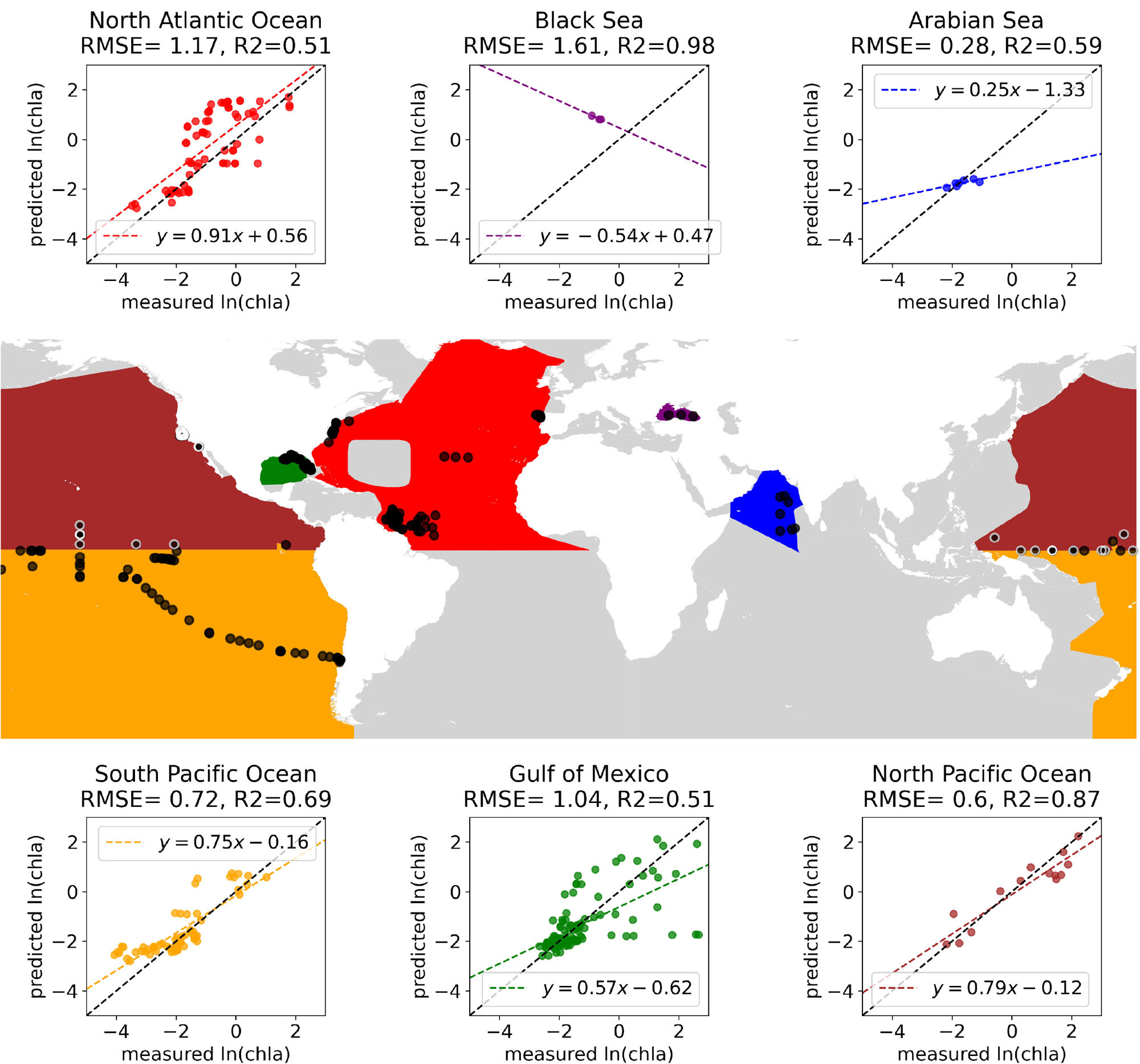
Spatial and temporal autocorrelation occurs when observations that are close together in space or time are more similar to each other than to those taken further apart. This autocorrelation is helpful for learning predictive models and interpolating data. However, if this autocorrelation is not accounted for in the dataset splits and evaluation protocol, there can be information leakage between training and test sets, causing overestimation of model performance because the test data are not independent from the training data (Figure 1). As an example, half of the irradiance data from ocean profiling floats comes from the Mediterranean (Begouen Demeaux and Boss, 2022), and if these data are simply split into a random training-validation-test subsets, the evaluation metrics could be substantially inflated by the autocorrelation in the data.

 

FIGURE 1. Using NOMAD (NASA bio-Optical Marine Algorithm Dataset), accuracy is achieved in predicting chl-a when a random forest model is trained on data from the North Pacific Ocean (black dots with white edges on the map) and then used for predictions based on data collected across a wide range of other locations (black dots). The model works well with data from the North Pacific and the South Pacific but has much lower and more variable accuracy for the North Atlantic and the Gulf of Mexico. > High res figure

 

If the intended use case of a model is to make predictions for observations acquired in a region or time period that was not present in training data, then train-validate-test splits should be designed to account for spatial or temporal autocorrelation (Rolf et al., 2024). ML evaluation protocols have been designed for this challenge in geospatial data such as spatial or temporal cross validation, checkerboard evaluation, and block or buffered cross validation (Rolf, 2023). A good design example would be: if the goal is temporal generalization, given a dataset of observations from 2010 to 2020, assign data from 2010 to 2015 to training, 2016 to 2018 to validation, and 2019 to 2020 to test (or better yet, do temporal cross validation). A bad design example would be: randomly split the data into train-​validate-​test following a standard 80/10/10% split in which data from all years can be in all subsets.

Sampling Strategies

The sampling strategies used to collect the labels that will comprise the test dataset are important to consider when trying to understand whether a test set is representative of a target population at model deployment time. Many in situ oceanographic datasets are collected using opportunistic sampling and are clustered in space and time (e.g., close to shore, rarely during winter storms). This results in a biased representation of the environment, which affects the accuracy estimation of the model, especially if spatial/temporal autocorrelation is not accounted for in evaluation. Begouen Demeaux et al. (2024) showed that a model estimating the diffuse attenuation coefficient trained on a large Biogeochemical Argo float dataset was still biased because it did not represent the real distribution of values in the ocean. Even if a probability sample (e.g., random uniform) is constructed to collect test data, sample size can greatly impact the uncertainty of the metric because it may miss rare or clustered patterns. For example, if a certain phytoplankton is rare, it may never appear in training data yet could still be encountered when the model is deployed (Nardelli et al., 2022). Thus, it is important to consider different sampling strategies and estimate standard errors/​confidence intervals of performance metrics when evaluating predicted products (Stehman and Foody, 2019).

ML models have no mechanistic representation of the ocean system. They are comprised of statistical relationships built using only the training data they have received. Given the many influences on the physical and biological states of the ocean, it can be hard to ensure proper training data across all relevant dimensions and conditions, particularly in higher dimensional spaces. Evaluating spatial and temporal generalizability and including anomaly detection tests can help resolve these issues.

Hypotheses and Physical Mechanisms Are Still Important in ML

Conducting data-driven science and exploration does not mean disregarding established knowledge of a system. Prediction should be combined with inference—understanding how the system works and making estimates either about future state or inverting parameters of interest. For example, in the western Atlantic, climatological wind speed may be connected to chl-a concentration through shared relationships with insolation and wind-driven mixing. However, this climatological wind and chl-a correlation does not mean that daily wind speed would be a good predictor of chl-a concentration in any causal way. As always, correlation does not imply causation, and the difference should be weighed when choosing model inputs and outputs.

While explorations of the entire dataset (e.g., via unsupervised methods for dimensionality reduction and visualization) and testing explanatory power via ML models may help form hypotheses, some understanding of the connections between the inputs and outputs of a model is typically warranted. ML can of course be used to gain insight into unexpected physical processes and guide the creation of effective physical relationships, but investigations into causation using more formal causal inference frameworks (i.e., Runge et al., 2019) are likely to both benefit the scientific process and guide model development through more informed model predictors and relationships.

Physically informed models with one to two expert-designed features may be much more generalizable and well constrained than ML models working on the raw data. In recent work predicting the diffuse attenuation coefficient from satellite ocean color, a simple analytical model developed from radiative transfer theory was shown to have less bias in an open-ocean environment than in an empirical approach. The empirical model, despite being tuned using a large global training dataset, had limited open ocean data, leading to greater bias in those regions (Begouen Demeaux et al., 2024).

Caveats of Complexity in an Uncertain Ocean

ML models are adept at modeling nonlinear transformations of input to output data, but we must consider the trade-offs between complexity and generalization. For example, is the community, and our own insight into the Earth system, better served by a complex ML model with high performance or a marginally lower scoring but simpler model, or potentially a much lower scoring but more generalizable mechanistic model? The answer will be different based on each project’s goals but should be considered. Here, we address two concerns in model development and deployment related to model complexity: uncertainty and anomalies.

Uncertainties

Incorporating uncertainty into model development and propagating uncertainty through to model predictions is critical for meaningful output (Elipot et al., 2022) as well as for performance evaluation. During model development, the uncertainty from each step must be understood and, during model use, the uncertainty from the input data must be propagated properly through the process.

Often during development, models are compared on the basis of accuracy (e.g., root mean square error, RMSE) without regard for uncertainty in input data (e.g., R_rs), label values (e.g., measured chl-a concentration), or—​importantly for small datasets—the uncertainty injected in the training/​testing data split. To objectively and robustly evaluate a model, all relevant uncertainties must be considered.

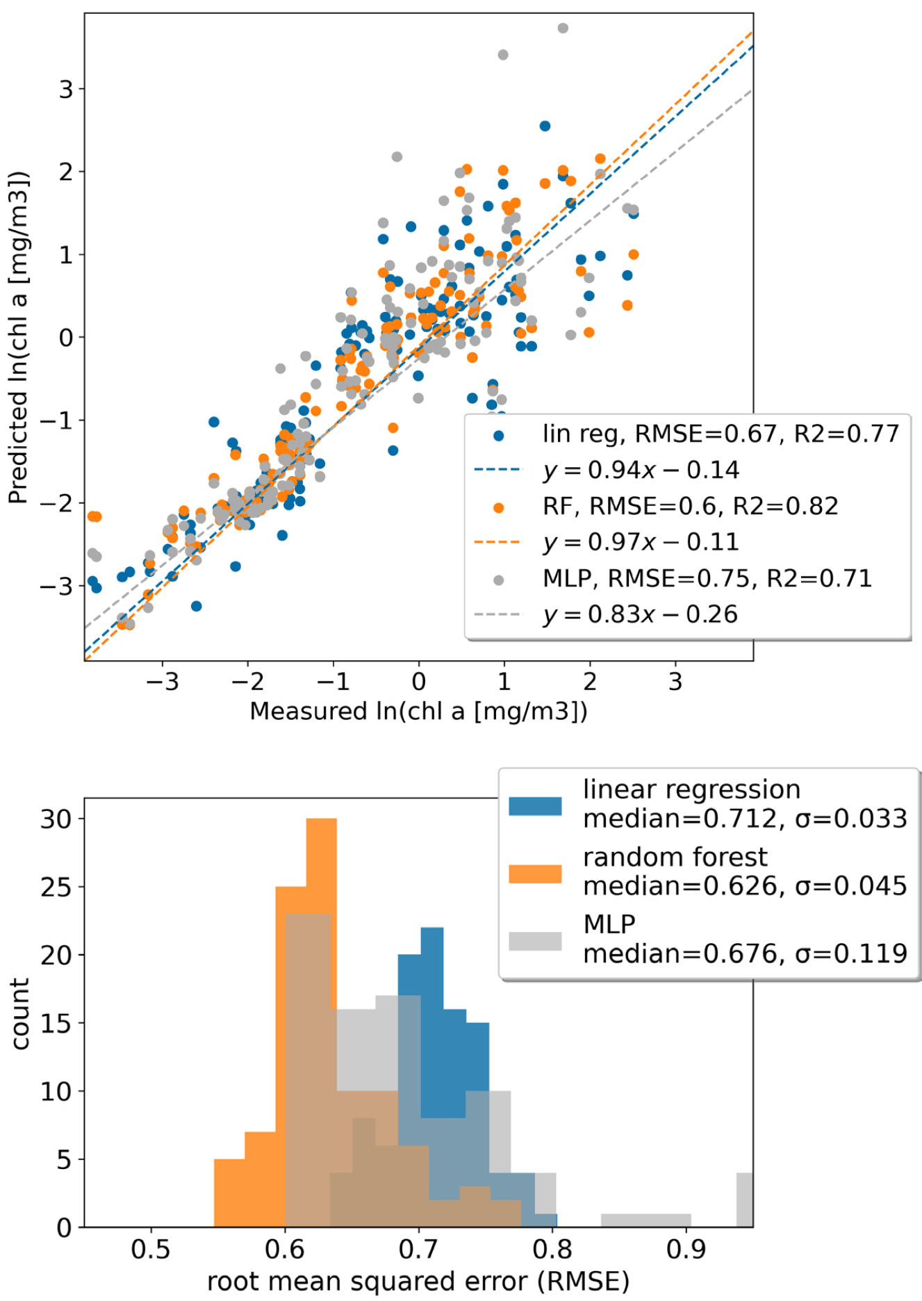
As a case study, consider three models of varying complexity for predicting chl-a from R_rs: a multiple linear regression, a random forest, and a multi-layer perceptron (MLP, a simple neural network) using the same data as in Figure 1. For a given train/test split and assuming all input and label measurements are exact, a specific model may appear more accurate (Figure 2, top panel). Yet, if we take a Monte Carlo approach and randomly shuffle the test/train splits and account for input and label uncertainty, it is not so clear (Figure 2, bottom panel). The uncertainty in the RMSE in this case is primarily driven by stochasticity in the train/test splits rather than in the measurement technique, which likely has to do with poor generalizability across regions or poor representation of water types. Striving to generate the best global algorithm might encourage collection or collation of more data rather than investing in more complex algorithm development for the existing data. This could also encourage different sampling approaches, such as more profiling floats vs. vessel-​based sampling. The ocean science community should follow the practice of the ML research community to report results using the mean and standard deviation over multiple random seeds and stratifying the test data over seasons and regions as described in Spatial and Temporal Autocorrelation below.

 

FIGURE 2. An example of three different algorithms of varying complexity trained to predict chl-a from remote sensing reflectance. (top panel) The dashed lines represent a regression between model predictions and measured in situ chl-a values and show the lowest root-mean-square-error (RMSE) is from the random forest model. (bottom panel) Distributions of RMSE for 100 different model training cycles accounting for the uncertainty in the radiometric measurement and the chl-a measurement by picking values from the distribution of expected values and randomly shuffling the training and testing data. When accounting for the full uncertainty, we cannot distinguish between the random forest and the multi-layer perceptron (MLP), yet some individual runs, such as in the top panel, may make it appear as if there is a substantial difference. > High res figure

 

Anomalies

Much of what we care about in the ocean, particularly in the context of climate change, involves anomalies and data points that lie outside the distribution of our training data. However, if not trained appropriately, ML models trained to predict phytoplankton types or harmful algal blooms may fail to detect these novel, significant events. As an example, imagine a model for predicting phytoplankton species from microscopy trained on all past images in a region. In the following year, a new phytoplankton species appears in the region, so that the model will never predict the correct class because it isn’t trained on this species. There are effective conventional statistical and ML approaches for anomaly detection (e.g., Isolation Forest, Local Outlier Factor), but they must be intentionally employed. The cost function of many models can also be modified to prioritize rare examples.

Dealing appropriately with rare examples and anomalies is particularly relevant given the long tail of ecological datasets (Van Horn and Perona, 2017), especially for phytoplankton (Nardelli et al., 2022). “Long tail” here describes the long-skewed distribution of rare species, rare spectra, rare combinations of sediment and minerals and phytoplankton types, all aspects that make traditional classification approaches challenging. These situations, where it is understood the training data cannot encompass all possible types encountered during model deployment, are sometimes called “open set” classification problems, and there is a rich literature not well explored in the ocean sciences (Geng et al., 2021).”

In sum, if a model is not properly evaluated, justified, and its limitations understood, releasing it into the wild or drawing conclusions from its predictions may in fact do a disservice to the community both through the opportunity cost of that time and effort and through adding a potentially poor model to an already cluttered landscape, obscuring better solutions and leading to poor inferences.

 

“If a model is not properly evaluated, justified, and its limitations understood, releasing it into the wild or drawing conclusions from its predictions may in fact do a disservice to the community…”

 

The Promise

Despite the caveats and complexities above, ML techniques have the potential to benefit the ocean sciences and the ocean remote sensing community. We strongly suggest that robustly evaluated supervised models, if proven to excel beyond existing baselines, paired with outlier detection to ensure inference is done within the testing distribution, can help advance many classification and regression problems. When simple or mechanistic models fail to capture complex relationships, it becomes useful to leverage the exceptional capabilities of ML.

A broad vision for machine learning in geosciences can be found in Tuia et al. (2021), who advocate for improved reasoning, multi-modal approaches, consistency with domain-specific knowledge (e.g., following physical equations), enhanced interpretability, and learning causal relationships. Rolf et al. (2024) present arguments and suggest pathways for machine learning researchers to consider satellite remote sensing data as a unique data modality for machine learning and to develop techniques that are uniquely suited to these data needs. Here, we lay out a vision for a range of other creative and currently underexplored applications specific to ocean remote sensing.

A Case Study on Unsupervised Exploration and Anomaly Detection

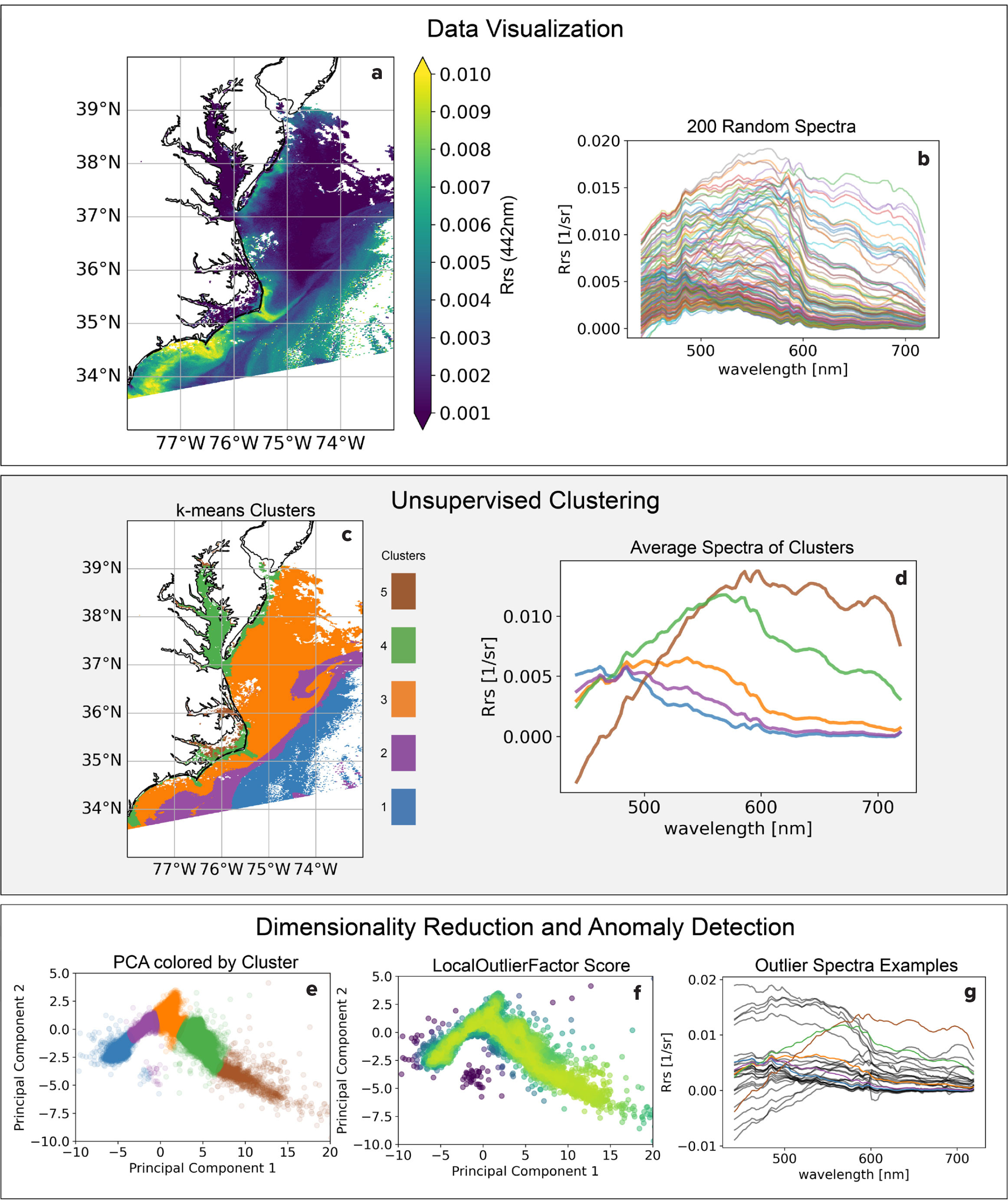
We illustrate the advantages of unsupervised learning and anomaly detection for dataset exploration by investigating an R_rs image from the recently launched PACE mission (Figure 3). This small subset of a single image contains >2,000,000 pixels, and each pixel represents 184 measurements across the spectrum from 350 nm to 700 nm. There is a large degree of spectral variability in this region ranging from open ocean to estuarine (Figure 3b). We map these spectra to five spatially coherent clusters using k-means clustering (Figure 3c,d). Viewing the data in a dimensionality reduced space via PCA, it is clear there is continuity between the clusters rather than their being discrete groups. This is often the case with ocean phenomena, and it warrants specific approaches. Using the anomaly detection algorithm LocalOutlierFactor from the scikit-learn library, we further investigate deviations from these clusters that may stem from atmospheric effects, high surface glint, or locally rare water column constituents. Simple ML-aided data exploration at the onset of a project can help users gain intuition for the dataset and develop informed hypotheses. See https://github.com/patrickcgray/ml_in_ocean_rs/blob/main/clustering_pace.ipynb for a step-by-step walk through.

 

FIGURE 3. A Plankton, Aerosol, Cloud, ocean Ecosystem (PACE) satellite mission image visualized as (a) Rrs(442 nm), (b) 200 randomly selected spectra showing the variability in the study region, (c) clusters via k-means shown geographically, and (d) the average spectra from each cluster. The bottom three graphs show data visualized by (e) the first two principal components colored by cluster, (f) LocalOutlierFactor anomaly score where the darker colors indicate more likely to be anomalous, and (g) highly anomalous spectra shown along with the five main clusters for reference. > High res figure

 

Self-Supervised Learning

The labeled data needed for supervised learning and evaluation is scarce and spatially clustered in ocean remote sensing. However, unlabeled data are plentiful—satellites acquire observations uniformly everywhere in the world at regular time intervals. Self-supervised learning (SSL) uses unlabeled data to construct a pre-text task (such as masked reconstruction) for conducting supervised learning. Using the SSL paradigm, models can be pre-trained using extremely large unlabeled ocean remote sensing datasets that could offer significant benefits for improving learning efficiency and accuracy in downstream tasks. Effectively leveraging SSL in ocean remote sensing requires investigating suitable pre-text tasks, including—but going beyond—masked reconstruction (Agabin and Prochaska, 2023). Future work should also investigate new approaches to model architectures, positional encoders, pre-training data curation, and other key elements of SSL methods that are uniquely suited to learning useful patterns in ocean remote sensing data. To help guide future work, the ocean remote sensing community should define which downstream tasks are most appropriate and informative for evaluating self-​supervised “foundation” models (e.g., by curating a suite of tasks like the terrestrial GeoBench; Lacoste et al., 2023).

Hybrid Physical Models

An emerging application of deep learning is to couple an ML model (e.g., a neural network) to a traditional numerical model of a physical process (e.g., climate modeling), termed a “hybrid physical model.” The core concept involves replacing complex, typically nonlinear processes in a mechanistic model with an ML approximator to enhance resolution or speed up the process. The ML emulator is trained on a set of expensive, high-resolution model runs representing the processes to be approximated. This has been used in ocean color remote sensing to speed up the retrieval of ocean properties. In one case, a neural network replaced the forward radiative transfer model and was able to be run 10³ times faster than the physical model in an iterative optimization approach (Gao et al., 2021). This approach bears the risk, however, of generalizing poorly, for example, generating highly erroneous results if presented with input parameters that lie far outside the training set. Furthermore, neural network-based emulators generally lack the physical intuition that one may implement with a heuristic algorithm. See Reichstein et al. (2019) for an overview of both opportunities and challenges for ML in Earth science and a specific focus on hybrid physical-DL models.

Bayesian Models

There are significant opportunities for the oceanographic community to further leverage Bayesian techniques combined with ML that have been applied extensively elsewhere. Most bio-optical inversion algorithms employ traditional linear regression algorithms, ignore measurement error, and don’t account for highly correlated uncertainties and retrieval targets. The Bayesian approach forces explicit identification and definition of priors that are typically present but unexplicit in frequentist approaches. In cases where a forward model can relate ocean properties to primary observables (e.g., a radiative transfer code linking absorption and backscattering to radiance measured by satellite), Bayesian inference techniques should be explored (e.g., Monte Carlo Markov chains, nested sampling). While computationally expensive, such methods already exist for atmospheric corrections and are under active development for inherent optical property retrievals (Prochaska and Frouin, 2024). Bayesian approaches have also shown promise in improving predictions for data undergoing distribution shifts (Seligmann et al., 2023), and there are mature tools for integrating deep learning with Bayesian methods (e.g., Tensorflow-Probability).

Data Manifolds

The apparent successes of DL in remote sensing indicates these models can effectively extract patterns from input data. Indeed, the lower dimensional data manifold embedding that is generated could become a basic object from which scientific inquiry is performed (Meilă and Zhang, 2024). Applications like these are already common in remote sensing studies on land (e.g., Tseng et al., 2023) and could translate well to ocean studies. In the ocean, physics-informed manifolds extract trends and non-correlations from complex datasets and can indicate regions of distinct dynamics (Sonnewald et al., 2019). These manifolds enable the investigation of physically similar but complex scenes and the classification or regression of dominant physical processes. We foresee an increasing emergence of the construction of data manifolds and analysis as the fundamental workflow of scientific discovery.

Data Integration

Another promising application of ML for ocean research is in facilitating the utilization of the large, disparate datasets collected from a variety of in situ platforms to complement remote-sensing data and enable algorithm development. While in situ data are abundantly and freely available, usage is hindered by the fact that data integration processes are currently performed manually, a tedious and grueling task that is not feasible for many large-scale studies. The improved ability of ML tools to extract knowledge from text and to use domain ontologies to integrate and align data opens the way for implementing tools for automating the ocean data integration process (e.g., the Ocean Data Integration Initiative, https://odini.net/; Sagi et al., 2020). Implementation of ML-based data integration tools will also help mitigate a primary challenge in remote sensing algorithm development—limited in situ data. For example, integrating all available flow cytometry datasets and pairing them with satellite ocean color data would allow more robust ML models to be developed for predicting phytoplankton type.

Spatial Features

While spatial (and temporal) features are not typically used in ocean remote sensing (e.g., ocean color where per-pixel per-image inversions are the norm), extracting features from spatial and temporal data and incorporating them into our inversions or using them as a new data stream may be a promising approach (Gray et al., 2024). This is one area where ML, and specifically DL, can be easily employed (e.g., convolutional neural networks or vision transformers). For ocean color research, we advocate beginning with simple, unsupervised algorithms to perform data exploration and then developing custom applications to meet scientific or community needs. Similar research is being pursued on sea surface temperature (e.g., Prochaska et al., 2023) and other parameters within the ocean remote-sensing community.

 

Conclusion

Our hope is to motivate the community to question the advantages and disadvantages of employing ML models to assist in answering geophysical questions. We emphasize caution when using supervised models in regions where there is limited confidence in the spatiotemporal comprehensiveness of the labeled data or in cases where anomalies are of interest. The nonlinear transformations done by many ML models are useful when playing to their strengths but can also hide trends and novel data. They should be used as specialized tools, not the initial hammers applied to every question. We emphasize that researchers should consider what they hope to learn before using ML tools. Is your objective the highest model prediction accuracy on a study region well defined by available training data? Do you seek broad Earth system understanding? Are you exploring unknown phenomena that don’t fit into a supervised model paradigm?

We suggest that in a changing world and a complex ocean system—with many degrees of freedom and nonlinear feedbacks—and with a lack of in situ data spanning all states of the ocean, a simpler and more physical model is generally better. Until collection of in situ data transitions beyond “grossly inadequate expeditionary sampling” and we can sample the ocean in all its states, interpolation methods are likely to err somewhere at some time, and we will miss key processes (Munk, 2002). There are many good reasons for using an ML model, but they must apply in each case where it is deployed and be worth the complexity, time, and effort.

We are likely to cross climate thresholds and ocean ecosystem tipping points in the next decade. The trainees of today will be the leading scientists as we pass these thresholds, as Earth experiences peak radiative forcing, including some of the most dramatic climate impacts. Improper usage of ML models could obscure these shifts and our understanding of them—or with proper use, they could help us understand, predict, and manage them.

 

Acknowledgments

We acknowledge support from the Zuckerman STEM Leadership Program to PCG. We thank three anonymous reviewers who considerably improved this article through their constructive feedback. We also thank members of the NASA Ocean Biology Processing Group for their effort to collate NOMAD (the NASA bio-Optical Marine Algorithm Dataset) and the NASA PACE Team for a huge effort to deliver data from the new mission, both of which are used here.

Data and Code Availability

All data and code to exactly recreate all figures and case studies can be accessed on Github at https://github.com/patrickcgray/ml_in_ocean_rs.

Gray, P.C., E. Boss, J.X. Prochaska, H. Kerner, C. Begouen Demeaux, and Y. Lehahn. 2024. The promise and pitfalls of machine learning in ocean remote sensing. Oceanography 37(3):52–63, https://doi.org/10.5670/oceanog.2024.511.

1. Agabin, A., and J.X. Prochaska. 2023. Reconstructing sea surface temperature images: A masked autoencoder approach for cloud masking and reconstruction. ArXiv, https://doi.org/10.48550/arXiv.2306.00835.
2. Begouen Demeaux, C., and E. Boss. 2022. Validation of remote-sensing algorithms for diffuse attenuation of downward irradiance using BGC-Argo floats. Remote Sensing 14(18):4500, https://doi.org/​10.3390/rs14184500.
3. Begouen Demeaux, C., E. Boss, J. Tan, and R. Frouin. 2024. Algorithms to retrieve the spectral diffuse attenuation coefficient of light in the ocean from remote sensing. Optics Express 32(2):2,507–2,526, https://doi.org/10.1364/OE.505497.
4. Bisson, K.M., P.J. Werdell, A.P. Chase, S.J. Kramer, B.B. Cael, E. Boss, and M.J. Behrenfeld. 2023. Informing ocean color inversion products by seeding with ancillary observations. Optics Express 31(24):40,557–40,572, https://doi.org/​10.1364/OE.503496.
5. Bzdok, D., N. Altman, and M. Krzywinski. 2018. Statistics versus machine learning. Nature Methods 15(4):233–234, https://doi.org/10.1038/nmeth.4642.
6. Cael, B.B., K. Bisson, E. Boss, and Z.K. Erickson. 2023. How many independent quantities can be extracted from ocean color? Limnology and Oceanography Letters 8(4):603–610, https://doi.org/​10.1002/lol2.10319.
7. Chase, A.P., E.S. Boss, N. Haëntjens, E. Culhane, C. Roesler, and L. Karp-Boss. 2022. Plankton imagery data inform satellite-based estimates of diatom carbon. Geophysical Research Letters 49(13):e2022GL098076, https://doi.org/​10.1029/2022GL098076.
8. Chollet, F. 2021. Deep Learning with Python, 2nd ed. Manning, 504 pp.
9. El Hourany, R., J. Pierella Karlusich, L. Zinger, H. Loisel, M. Levy, and C. Bowler. 2024. Linking satellites to genes with machine learning to estimate phytoplankton community structure from space. Ocean Science 20(1):217–239, https://doi.org/​10.5194/os-20-217-2024.
10. Elipot, S., K. Drushka, A. Subramanian, and M. Patterson. 2022. Overcoming the challenges of ocean data uncertainty. Eos 103, https://doi.org/​10.1029/2022EO220021.
11. Gao, M., B.A. Franz, K. Knobelspiesse, P.-W. Zhai, V. Martins, S. Burton, B. Cairns, R. Ferrare, J. Gales, O. Hasekamp, and others. 2021. Efficient multi-​angle polarimetric inversion of aerosols and ocean color powered by a deep neural network forward model. Atmospheric Measurement Techniques 14(6):4,083–4,110, https://doi.org/​10.5194/amt-14-4083-2021.
12. Geng, C., S.-J. Huang, and S. Chen. 2021. Recent advances in open set recognition: A survey. IEEE Transactions on Pattern Analysis and Machine Intelligence 43(10):3,614–3,631, https://doi.org/​10.1109/TPAMI.2020.2981604.
13. Gray, P.C., E. Boss, G. Bourdin, Mission Microbiome AtlantECO, Tara Pacific Consortium, and Y. Lehahn. 2024. Emergent patterns of patchiness reflect decoupling between ocean physics and biology. BioRxiv, https://doi.org/10.1101/2024.05.24.595779.
14. Hogg, D.W., and S. Villar. 2024. Is machine learning good or bad for the natural sciences? ArXiv, https://doi.org/10.48550/arXiv.2405.18095.
15. Irisson, J.-O., S.-D. Ayata, D.J. Lindsay, L. Karp-Boss, and L. Stemmann. 2022. Machine learning for the study of plankton and marine snow from images. Annual Review of Marine Science 14(1):277–301, https://doi.org/10.1146/annurev-marine-041921-013023.
16. Jamet, C., H. Loisel, and D. Dessailly. 2012. Retrieval of the spectral diffuse attenuation coefficient K_d(λ) in open and coastal ocean waters using a neural network inversion. Journal of Geophysical Research: Oceans 117(C10), https://doi.org/​10.1029/​2012JC008076.
17. Jönsson, B.F., J. Salisbury, E.C. Atwood, S. Sathyendranath, and A. Mahadevan. 2023. Dominant timescales of variability in global satellite chlorophyll and SST revealed with a MOving Standard deviation Saturation (MOSS) approach. Remote Sensing of Environment 286:113404, https://doi.org/10.1016/j.rse.2022.113404.
18. Lacoste, A., N. Lehmann, P. Rodriguez, E.D. Sherwin, H. Kerner, B. Lütjens, J.A. Irvin, D. Dao, H. Alemohammad, A. Drouin, and others. 2023. GEO-Bench: Toward foundation models for Earth monitoring. ArXiv, https://doi.org/10.48550/arXiv.2306.03831.
19. Lecun, Y., Y. Bengio, and G. Hinton. 2015. Deep learning. Nature 521(7553):436–444, https://doi.org/​10.1038/nature14539.
20. Meilă, M., and H. Zhang. 2024. Manifold learning: What, how, and why. Annual Review of Statistics and Its Application 11(1):393–417, https://doi.org/​10.1146/annurev-statistics-040522-115238.
21. Munk, W. 2002. The evolution of physical oceanography in the last hundred years. Oceanography 15(1):135–141, https://doi.org/​10.5670/oceanog.2002.45.
22. Nardelli, S.C., P.C. Gray, and O. Schofield. 2022. A convolutional neural network to classify phytoplankton images along the West Antarctic Peninsula. Marine Technology Society Journal 56(5):45–57, https://doi.org/10.4031/MTSJ.56.5.8.
23. O’Reilly, J.E., and P.J. Werdell. 2019. Chlorophyll algorithms for ocean color sensors - OC4, OC5 & OC6. Remote Sensing of Environment 229:32–47, https://doi.org/10.1016/j.rse.2019.04.021.
24. Pahlevan, N., B. Smith, J. Schalles, C. Binding, Z. Cao, R. Ma, K. Alikas, K. Kangro, D. Gurlin, N. Hà, and others. 2020. Seamless retrievals of chlorophyll-a from Sentinel-2 (MSI) and Sentinel-3 (OLCI) in inland and coastal waters: A machine-learning approach. Remote Sensing of Environment 240:111604, https://doi.org/10.1016/j.rse.2019.111604.
25. Prochaska, J.X., E. Guo, P.C. Cornillon, and C.E. Buckingham. 2023. The fundamental patterns of sea surface temperature. IEEE Transactions on Geoscience and Remote Sensing 61:1–19, https://doi.org/​10.1109/TGRS.2023.3300272.
26. Prochaska, J.X., and R.J. Frouin. 2024. On the peril of inferring phytoplankton properties from remote-​sensing observations. ArXiv, https://doi.org/​10.48550/arXiv.2408.06149.
27. Reichstein, M., G. Camps-Valls, B. Stevens, M. Jung, J. Denzler, N. Carvalhais, and Prabhat. 2019. Deep learning and process understanding for data-driven Earth system science. Nature 566(7743):195–204, https://doi.org/10.1038/s41586-019-0912-1.
28. Ridge, J.T., P.C. Gray, A.E. Windle, and D.W. Johnston. 2020. Deep learning for coastal resource conservation: Automating detection of shellfish reefs. Remote Sensing in Ecology and Conservation 6(4):431–440, https://doi.org/​10.1002/rse2.134.
29. Rolf, E. 2023. Evaluation challenges for geospatial ML. ArXiv, https://doi.org/10.48550/arXiv.2303.18087.
30. Rolf, E., K. Klemmer, C. Robinson, and H. Kerner. 2024. Mission critical—Satellite data is a distinct modality in machine learning. ArXiv, https://doi.org/​10.48550/arXiv.2402.01444.
31. Runge, J., S. Bathiany, E. Bollt, G. Camps-Valls, D. Coumou, E. Deyle, C. Glymour, M. Kretschmer, M.D. Mahecha, J. Muñoz-Mari, and others. 2019. Inferring causation from time series in Earth system sciences. Nature Communications 10(1):2553, https://doi.org/10.1038/s41467-019-10105-3.
32. Sagi, T., Y. Lehahn, and K. Bar. 2020. Artificial intelligence for ocean science data integration: Current state, gaps, and way forward. Elementa: Science of the Anthropocene 8:21, https://doi.org/10.1525/elementa.418.
33. Sauzède, R., H. Claustre, J. Uitz, C. Jamet, G. Dall’Olmo, F. D’Ortenzio, B. Gentilli, A. Poteau, and C. Schmechtig. 2016. A neural network-​based method for merging ocean color and Argo data to extend surface bio-optical properties to depth: Retrieval of the particulate backscattering coefficient. Journal of Geophysical Research: Oceans 121(4):2,552–2,571, https://doi.org/​10.1002/2015JC011408.
34. Seligmann, F., P. Becker, M. Volpp, and G. Neumann. 2023. Beyond deep ensembles: A large-scale evaluation of Bayesian deep learning under distribution shift. ArXiv, https://doi.org/10.48550/arXiv.2306.12306.
35. Sonnewald, M., C. Wunsch, and P. Heimbach. 2019. Unsupervised learning reveals geography of global ocean dynamical regions. Earth and Space Science 6(5):784–794, https://doi.org/​10.1029/​2018EA000519.
36. Stehman, S.V., and G.M. Foody. 2019. Key issues in rigorous accuracy assessment of land cover products. Remote Sensing of Environment 211:111199, https://doi.org/10.1016/j.rse.2019.05.018.
37. Stock, A., A. Subramaniam, G.L. Van Dijken, L.M. Wedding, K.R. Arrigo, M.M. Mills, M.A. Cameron, and F. Micheli. 2020. Comparison of cloud-filling algorithms for marine satellite data. Remote Sensing 12(20):3313, https://doi.org/​10.3390/rs12203313.
38. Taori, R., A. Dave, V. Shankar, N. Carlini, B. Recht, and L. Schmidt. 2020. Measuring robustness to natural distribution shifts in image classification. ArXiv, https://doi.org/10.48550/arXiv.2007.00644.
39. Tseng, G., R. Cartuyvels, I. Zvonkov, M. Purohit, D. Rolnick, and H. Kerner. 2023. Lightweight, pre-trained transformers for remote sensing timeseries. ArXiv, https://doi.org/10.48550/arXiv.2304.14065.
40. Tuia, D., R. Roscher, J.D. Wegner, N. Jacobs, X. Zhu, and G. Camps-Valls. 2021. Toward a collective agenda on AI for Earth science data analysis. IEEE Geoscience and Remote Sensing Magazine 9(2):88–104, https://doi.org/10.1109/MGRS.2020.3043504.
41. Van Horn, G., and P. Perona. 2017. The devil is in the tails: Fine-grained classification in the wild. ArXiv, https://doi.org/10.48550/arXiv.1709.01450.

This is an open access article made available under the terms of the Creative Commons Attribution 4.0 International License (https://creativecommons.org/licenses/by/4.0/), which permits use, sharing, adaptation, distribution, and reproduction in any medium or format as long as users cite the materials appropriately, provide a link to the Creative Commons license, and indicate the changes that were made to the original content. Images, animations, videos, or other third-party material used in articles are included in the Creative Commons license unless indicated otherwise in a credit line to the material. If the material is not included in the article’s Creative Commons license, users will need to obtain permission directly from the license holder to reproduce the material.