Introduction
In 2012, the international GEOTRACES program (Anderson and Henderson, 2005; GEOTRACES Planning Group, 2006; SCOR Working Group, 2007; Frank et al., 2003; Anderson et al., 2014; Anderson, 2024, in this issue; https://www.geotraces.org/) decided to create and release a series of intermediate data products and to make these data publicly available to scientists and the interested general public. The main motivation was to not wait until the end of the program to issue a final data product but rather to create and release observational, analysis, and synthesis data products during the active program. By releasing and sharing data at early stages, GEOTRACES intends to strengthen and intensify collaboration within the geochemical community itself and also to attract and invite colleagues from other communities, such as physical, biological, and paleo oceanography, as well as modeling, to apply their unique knowledge and skills to marine biogeochemical research questions. To ensure the highest possible data quality and compatibility of the data submitted by different laboratories worldwide, GEOTRACES has from the beginning invested enormously in standardization and intercalibration efforts. These efforts were coordinated and overseen by the Standards and Intercalibration Committee (Aguilar-Islas, 2024, in this issue).
To this date, GEOTRACES has released three intermediate data products (IDPs): (1) IDP2014 (Mawji et al., 2015), (2) IDP2017 (Schlitzer et al., 2018), and (3) IDP2021 (original release: GEOTRACES Intermediate Data Product Group, 2021; version 2 update: GEOTRACES Intermediate Data Product Group, 2023). With each new release and update, there were significant increases in the numbers of data values, parameters, and data types included in the product. Geographical and temporal coverage also increased significantly each time. While the first data product, IDP2014, was mostly confined to the Atlantic Ocean, the latest product, IDP2021v2, now exhibits good data coverage in all ocean basins, including the Mediterranean, the Black Sea, and the Arctic Ocean (Figure 1).
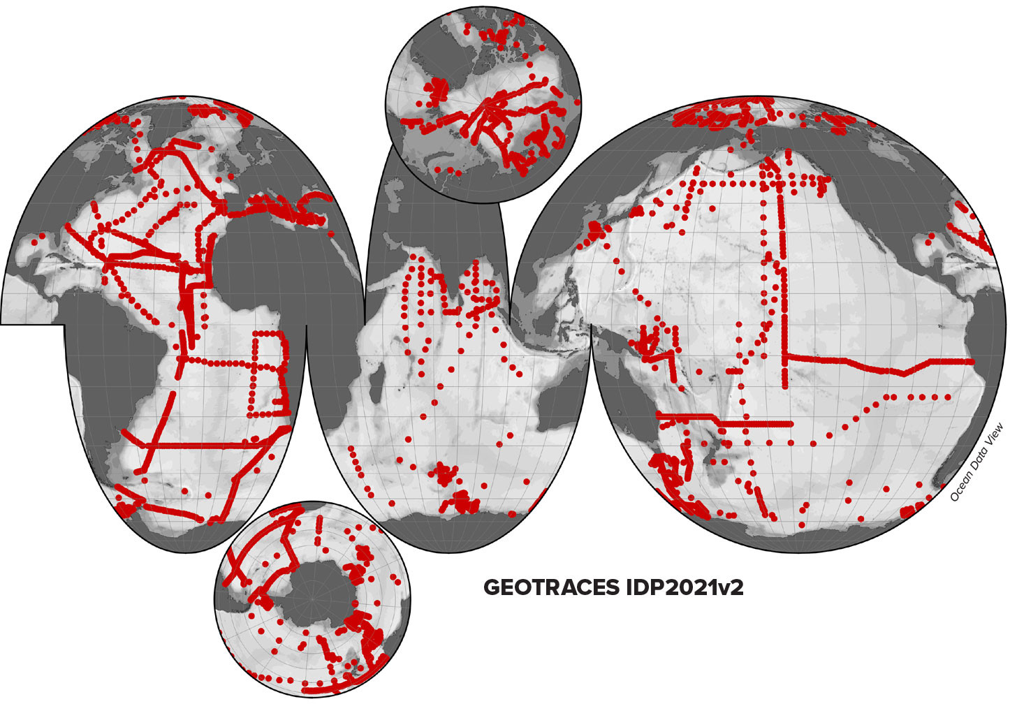
FIGURE 1. Map of seawater discrete sample stations in the GEOTRACES Intermediate Data Product 2021v2. > High res figure
|
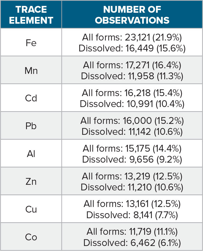
IDP2021v2 consists of five separate datasets: (1) seawater discrete sample data, (2) seawater CTD sensor data, (3) aerosol data, (4) precipitation data, and (5) data for snow and ice. The seawater discrete sample dataset is the core of the IDP and contains data for 586 parameters at 3,362 stations covering all ocean basins (Figure 1). GEOTRACES has created its own parameter-naming conventions, as described by Schlitzer et al. (2018). Table 1 shows the number of available data values for selected GEOTRACES trace elements that play important roles in a wide range of biogeochemical processes, including fixation of carbon and silicate, calcification, nitrification/denitrification, and the remineralization of organic matter. While at the beginning of GEOTRACES only a few hundred contamination-free data values existed for Fe and Zn (Anderson et al., 2014a), IDP2021v2 now provides more than 23,000 values for Fe and between 13,000 and 17,000 values for the other selected trace elements. This wealth of data allows, for the first time, the detailed mapping of trace element distributions in the entire world ocean.
TABLE 1. Number of measurements of selected GEOTRACES trace elements in the IDP2021v2 seawater discrete sample dataset. Numbers in parentheses indicate the percentage of discrete samples that contain data for that parameter. The “All forms” values include dissolved as well as particulate measurements. For Fe, this also includes data for Fe_II and soluble Fe. > High res table
|
In addition to the actual measurements, the GEOTRACES IDPs also contain extensive metadata on all the parameters measured on all GEOTRACES cruises, including ship operations, sampling procedures, analytical measurement techniques, calibration methods, names of the investigators making the measurements, and also references to original publications related to the observations. All this information is crucially important for correct interpretation and assessments of the GEOTRACES data nowadays and, even more importantly, in the future. Obtaining contamination-free samples and high-quality, calibrated trace elements and isotope (TEI) data values is still a challenge that requires expert skills available in only a relatively small number of laboratories worldwide. Sampling and measurement procedures for many TEIs still vary among laboratories, and it is fundamentally important to document the actual procedures used. Inclusion of investigator names in the IDP as well as on the eGEOTRACES visuals is a way of acknowledging and recognizing the fundamental work of the more than 370 data creators involved in the IDPs. The GEOTRACES IDPs would not exist without their willingness to contribute and share their data. The dynamic publication database incorporated in the IDPs makes it easy for data users to identify and cite the original publications associated with the data they use or to consider initiating collaborations with the data originators.
Unlike previous IDP versions that required users to register and log in before they could download the digital data, IDP2021 now provides free and anonymous access, but requires users to accept and adhere to the GEOTRACES Fair Data Use Agreement (https://egeotraces.org/docs/IDP2021_FairDataUseStatement.pdf). In essence, this agreement requires users to acknowledge the contributions of GEOTRACES investigators and data providers through invitations to coauthorship and/or by citing relevant original scientific articles and the IDP2021 itself.
The IDP2021v2 digital data are available for download as large, complete packages at http://www.bodc.ac.uk/geotraces/data/idp2021/. Users can also retrieve customized subsets of the data for smaller domains, individual cruises, or specific parameter sets via an online data extraction service at https://geotraces.webodv.awi.de/. Here, we will focus on how the rich IDP data resources can be accessed and utilized effectively using online analysis and visualization services. No data need to be downloaded and no special software needs to be installed by the user. We will also demonstrate how easy it is to access the rich metadata, such as cruise reports, documents on analytical procedures, names of data creators, and publication references. All these documents are just one or two mouse clicks away.
Important note on browser settings: Some features described below, such as downloading images, videos, or digital data, or clicking links or info buttons inside the webODV browser window, require that downloads as well as popup windows are enabled in your browser. Please see your browser documentation for instructions on how to do this.
eGEOTRACES Electronic Atlas
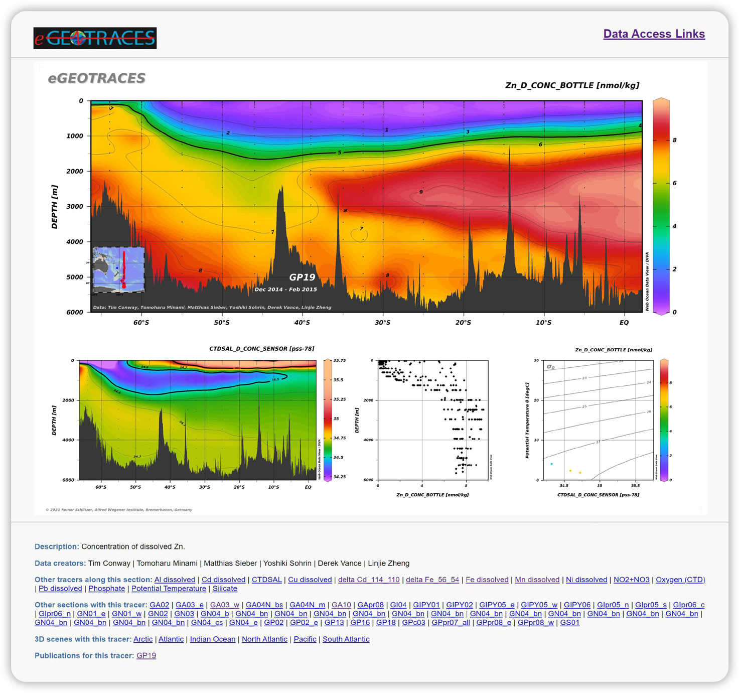
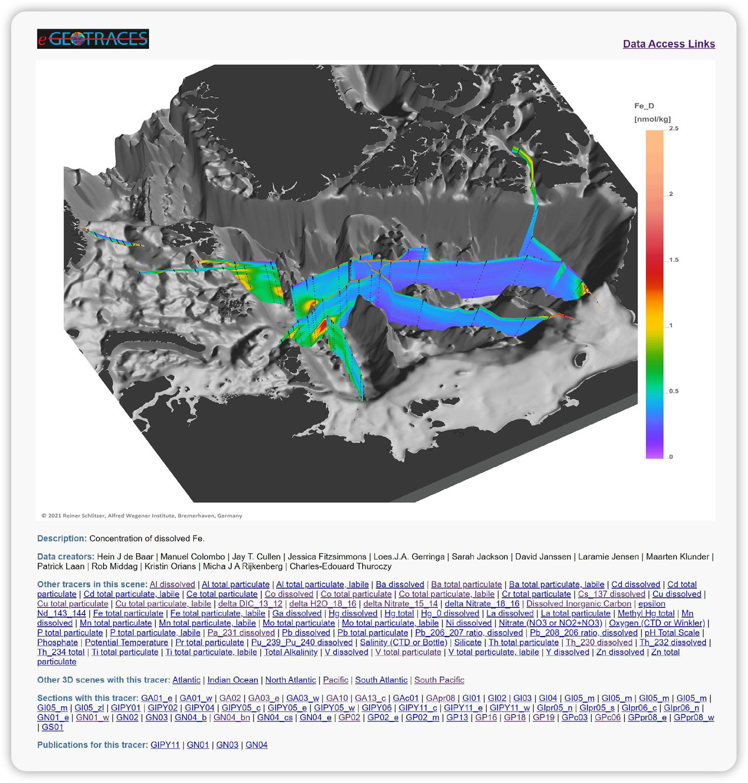
The eGEOTRACES Electronic Atlas is the visual component of IDP2021v2 and contains 1,463 section plots as well as 269 animated three-dimensional (3D) scenes for many (but not all) of the parameters in IDP2021v2. All plots are based on the digital data in IDP2021v2, with data values flagged as questionable/suspect or bad filtered out and not used for the plots. The eGEOTRACES website https://egeotraces.org/ provides a dynamic map where users start by selecting a data group and a tracer of interest. All GEOTRACES sections that contain a plot for the selected tracer are highlighted in red on the map, and basins containing a 3D animation for the selected tracer are highlighted in blue. Clicking on a red section label or a blue basin label will show the respective section plot or play the respective 3D scene. Example eGEOTRACES section and 3D scene pages are shown in Figures 2 and 3. Please note that all section plots and 3D scenes show the names of scientists who produced or are responsible for the data. Links to original publications related to the data can be found in the bottom line. This makes it easy for users to identify and acknowledge data producers. Clicking on Data Access Links in the upper right corner takes users to the IDP2021v2 download site and to the online subsetting and analysis services described below.
|
|
Clicking on a section plot loads a high-resolution version of the image. This can be downloaded and saved for use in one’s own publications, presentations, or outreach material. Use the browser’s Back button to return to the original section page. When viewing a 3D animation, move the mouse over the 3D scene to obtain an option bar that allows stopping the animation and positioning the view at arbitrary angles. Most browsers also allow download of a 3D movie file. Please note that downloaded eGEOTRACES videos are saved as webm files, which might not be supported by all video players or browsers.
All section and 3D animation pages include descriptions of the visualized parameters and lists of data creator names. In addition, there are groups of links to other section plots and 3D animations, including (1) links to other tracers along the particular section or in the scene, (2) other 3D scenes for the same tracer, and (3) other sections or 3D scenes for the given tracer. All these links greatly facilitate switching between and comparing different tracers along sections or in 3D scenes. All section plots use the same window layout geometries, and the different windows perfectly match when switching between tracers.
Section and 3D scene pages also contain links to the original publications associated with the selected tracer and section at the bottom of the page. Clicking on these links shows the list of publications from the dynamically updated reference database maintained at the GEOTRACES International Project Office (https://www.geotraces.org/geotraces-publications-database/).
The eGEOTRACES 3D scenes provide geographical and bathymetric context crucial for identifying tracer plume origins and extents and for inferring processes acting on the tracers and shaping their distributions. In addition to scientific usage, the interactive eGEOTRACES atlas and its visuals are great resources for teaching and outreach material. The 3D animations are easy for anyone to view and understand, and are useful for conveying societally relevant scientific results to interested non-scientists and policymakers.
Images and 3D movies from the eGEOTRACES atlas can be used free of charge for non-commercial purposes, such as in scientific publications, posters, presentations, and teaching activities, as long as the source is cited as follows: Schlitzer, R., eGEOTRACES – Electronic Atlas of GEOTRACES Sections and Animated 3D Scenes, http://egeotraces.org, 2021. High-resolution images are available on request.
IDP Digital Data Analysis
All five digital IDP2021v2 datasets are available for online analysis and visualization at the webODV Explore site https://explore.webodv.awi.de. In the following, we discuss only the seawater discrete sample dataset, the core of the IDP. We describe how the webODV browser interface can be used effectively to analyze and visualize IDP data online. We focus on the marine Zn cycle and on correlations of Zn with macronutrients, such as silicate and phosphate. Based on GEOTRACES IDP and earlier data, a near linear relationship between Zn and silicate was found (Bruland et al., 1978; Conway and John, 2014; Wyatt et al., 2014; Vance et al., 2017; Sieber et al., 2023). This is surprising given that synchrotron X-ray fluorescence analysis of individual phytoplankton cells showed that Zn was co-located with phosphorous (Twining and Baines, 2013), and remineralization of Zn together with phosphate would be expected, which would lead to good correlation of Zn with phosphate but not with silicate.
In the following, we provide hands-on descriptions and invite interested readers to follow step by step to create their own target plots. You will learn how to create correlation plots between Zn and the macronutrients silicate and phosphate, and obtain least-squares line fits for the Zn versus silicate case. Using specific formulas for Zn*, you will also learn how to establish expression-derived variables and show their distributions along GEOTRACES sections.
Basic features, such as obtaining data availability information, accessing the rich metadata, exporting selected data, and customizing eGEOTRACES section plots are explained first. Then we describe two use cases and provide detailed, hands-on instructions.
To start, visit the webODV Explore website https://explore.webodv.awi.de, navigate to Ocean > tracer > geotraces > idp2021 > seawater and click on the v2 version of the seawater discrete sample dataset (first entry). Alternatively, use the direct link to this dataset https://explore.webodv.awi.de/ocean/tracer/geotraces/idp2021/seawater/.
First-time visitors will see the Fair Data Use Agreement described above. You must agree before you can proceed. A new tab will open in your web browser showing a large station map of the dataset (if you are a first-time visitor), or the window layout (view) that existed when you closed your previous session. The user interface running in your web browser (called ODV-online) has been designed to mimic the user interface of the popular Ocean Data View (ODV) software (https://odv.awi.de). If you have used ODV before, you should feel at home right away and be productive from the start. If you have never used ODV, please read the Getting Started (https://odv.awi.de/fileadmin/user_upload/odv/docs/ODV-online_getting_started.pdf) and HowTo documents (https://odv.awi.de/fileadmin/user_upload/odv/docs/ODV-online_how-to.pdf).
Basics
The basic guidelines for using ODV-online are: (1) Left mouse clicks select stations or samples (making them current station or current sample). (2) Right-clicks open context sensitive menus that provide rich functionality, depending on the clicked object. For instance, right-clicking on the station map and choosing Save As Interrupted Map will generate a station map image similar to Figure 1. In addition to the context-sensitive menus, there is the main menu on the right side of the title bar. Current station and current sample are marked with red crosses on the map and the data plots. The metadata of the current station are shown in the current station list on the upper right side. Data values, data standard deviations (if available), and quality flag values, as well as info symbols ⓘ (if available) for the current sample are shown in the current sample list (middle/right). The color of a data value reflects its quality status: green indicates good data, red indicates questionable or bad data, and black indicates that no quality assessment was performed.
Obtaining Data Inventory Information
The seawater dataset contains measurements for a total of 586 parameters; however, most GEOTRACES sections or process studies contain data for a far smaller number of parameters. To quickly obtain lists of data counts available for the current cruise or current station (selected by left-clicking on a station on the map), right-click on an arbitrary parameter name in the current sample list (middle part of the menu at the right of the page) and choose Data Availability > Current Cruise or Data Availability > Current Station. Alternatively, use Collection > Browse Inventory > By Cruise and Variable to download an inventory summary for the entire dataset as well as for individual cruises.
Exporting Selected Data
As demonstrated by the use cases below, creation of publication-ready visuals normally does not require IDP data download to the user’s computer. However, to support special data analysis procedures not provided by webODV, users can export the original IDP data for user selected subsets of stations and parameters using the Export > Data options. Users can also download the X, Y, Z data of specific data windows via Export > Window Data.
Customizing eGEOTRACES Sections
The seawater dataset includes all 1,583 setups (views) used to create the static eGEOTRACES section plots (see above). For an easy start, you can enter a live data session with your favorite parameter and section using View > Load View. Then click on the respective GEOTRACES section and select your favorite parameter. For instance, choosing GP19_Zn_D_CONC_BOTTLE will reproduce Figure 2. You can customize the view by adapting the visual appearance, zooming into specific value ranges of interest, or selecting other parameters on the X, Y, or Z axes of the individual data plots.
Browsing Metadata Information
Detailed station and cruise metadata for the current station are shown in the top-right list window. In addition to the position and date/time of occupation, this includes operator’s cruise name, cruise start/end dates, chief and GEOTRACES scientist names, cruise alias names (if available), and, most importantly, a link to detailed cruise information documents. Simply click on the link shown in blue to view the cruise summary report. Note that popup windows need to be enabled in your browser. For most cruises, you will also find further links to cruise reports and track charts at the bottom of the page.
Detailed meta information about a particular data value in one of the data plots (e.g., Zn_D_CONC_BOTTLE) can be obtained by left-clicking on that data point in the plot to make it the current sample. Then scroll the current sample list and click on the info symbol ⓘ of the parameter of interest, for example, Zn_D_CONC_BOTTLE. Again, make sure that popup windows are enabled. A new browser tab will open and display a description of the parameter, the list of data creator names, a link to the analytical methods document as well as a link to publication references related to this value.
Use Case 1: Correlations Between Zn and Macronutrients
We now describe the specific steps necessary to create Figure 4, which contains correlation plots of Zn concentration versus silicate and phosphate for IDP2021v2 Zn data in the Atlantic Ocean. To provide a well-defined start, please choose option View > Load View and select AllStationsMap at the bottom of the public branch.
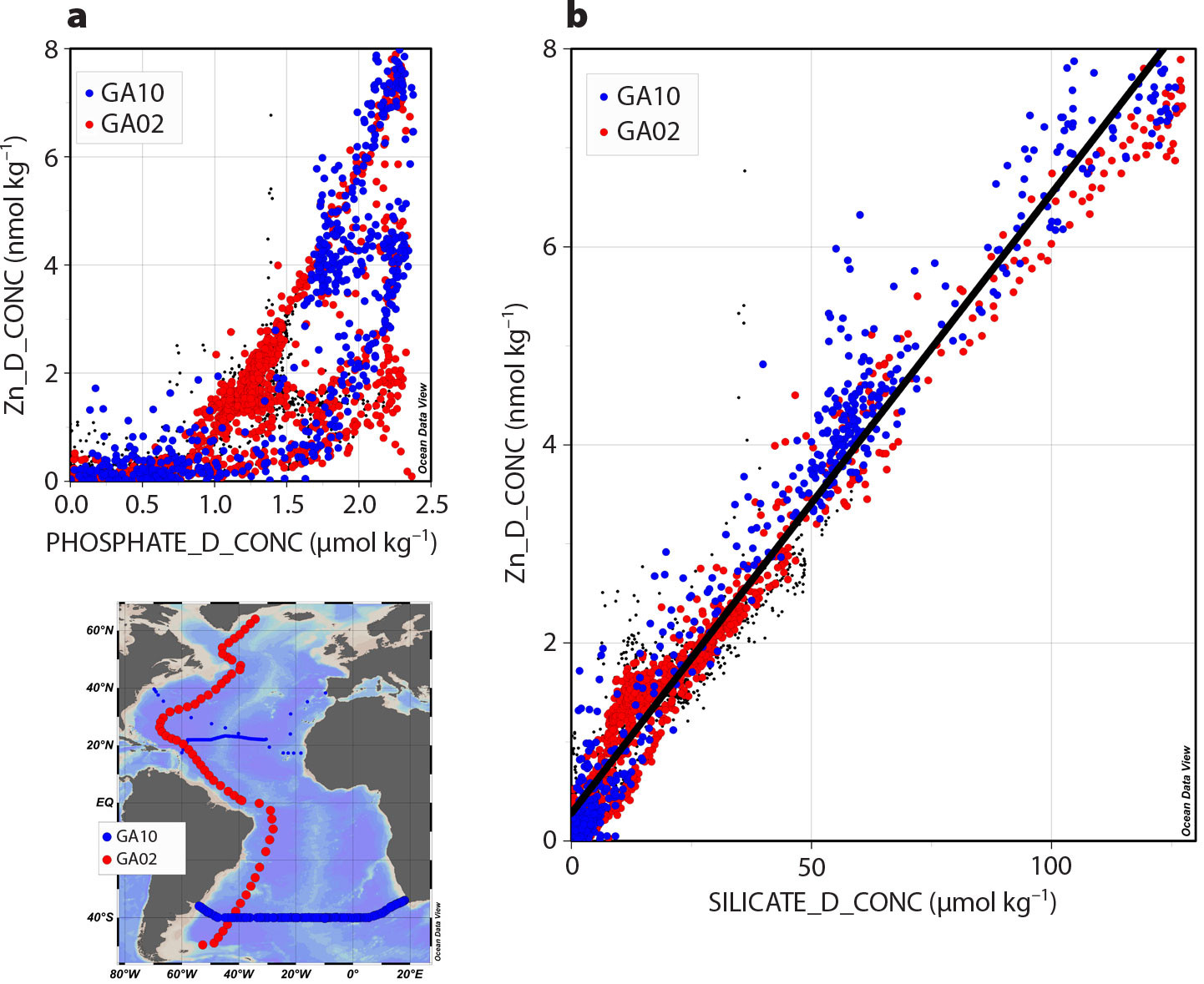
FIGURE 4. Correlation of Zn concentration versus (a) phosphate and (b) silicate using all IDP2021v2 Zn data from sections GA02, GA03, GA10, and GApr08. Note that most GA03 and GApr08 data (black dots) are hidden beneath the highlighted GA02 and GA10 values. > High res figure
|
Defining Aggregated Derived Variables
A variety of different sampling systems is used during GEOTRACES cruises, such as (a) Niskin or similar water sampling bottles, (b) trace-metal-clean towed surface samplers, (c) in situ or on-deck pumps, (d) pumps on an ice floe, and (e) ships’ underway surface seawater systems. Data arising from these different sampling methods are reported in separate parameters with name suffixes (a) BOTTLE, (b) FISH, (c) PUMP, (d) SUBICE_PUMP, and (e) UWAY. This separation makes it easy to analyze data from a specific sampling system and exclude the others. However, most of the time, it would be preferable to combine all measurements of a given TEI or hydrographic parameter, irrespective of the sampling method. For instance, when correlating Zn with silicate (see below), we would like to use all available Zn and silicate values from all sampling systems, BOTTLE, FISH, PUMP, SUBICE_PUMP, and UWAY, together in a single graph.
In order to accomplish this, we will define aggregated derived variables and use these on the X and Y axis of the correlation plots. Derived variables are requested via the View > Derived Variables option. In the Choices list on the right, click on Special, then on Aggregated Variable. Next, select all individual parameters that should be combined into a single parameter. For aggregated silicate, select variables 39, 54, 59, and 68; for aggregated phosphate, use 37, 53, 57, and 67; and for aggregated Zn, use 111, 131, 145, and 157. Be sure to hold down the control key when multi-selecting. Then adjust the label of the new aggregated derived variable by removing Aggregated from the beginning and _BOTTLE from the end. A parameter name without the sampling system suffix, such as Zn_D_CONC, then represents an aggregated derived variable that combines measurements of all selected sampling systems. Once defined, derived variable values appear at the end of the current sample list (middle right).
Saving Private Views
After you have made changes, such as defining derived variables or modifying the window layouts, you should regularly save the current settings using the View > Save View As option. Your settings are recorded as a private view; please take your time and choose a descriptive name. Later, you can load saved views via View > Load View. Please note that your private views are stored locally in your web browser. Use the View > Manage Resources > Views option to download your private views to .xview files before deleting browser data; otherwise, your private settings will be lost.
Defining Station Filters
By clicking on View > Station Filter > Customize, you can establish a large variety of conditions for accepting or rejecting stations. Only stations satisfying the specified conditions pass the station filter and are shown on the map. Only data from these stations are shown in data windows. Here, we want to filter for stations containing Zn data (any sampling system) and bearing specific cruise names.
Start by clicking on the Availability tab on the Station Filter dialog and select Zn variables 111, 131, 145, and 157, then select OR logic and press Apply. Only 893 out of 3,362 stations are now shown; each one of these stations is guaranteed to have Zn data. Now let’s continue filtering and only accept stations from specific cruises. Use View > Station Filter > Customize again and click the Name / Range tab. In the cruise label field, enter GA10 || GA02 || GA03 || GApr08 and press Apply. Now just 324 stations satisfy the station filter conditions, and only data from these stations will be shown in subsequently defined data plots. Finally, right-click on the map, choose Zoom, and slide the lines to crop the map and select the Atlantic sub-domain covered by stations.
Changing the Window Layout
Using option View > Layout Templates > 2 SCATTER Windows, we are now establishing a new window layout containing two SCATTER windows in addition to the station map. Note that SCATTER windows show all data of all stations in the map. Right-click on the large SCATTER window on the right, choose X-Variable, and select the previously defined variable SILICATE_D_CONC (near the bottom of the list). Then choose Y-Variable and select Zn_D_CONC. Repeat this procedure for the smaller SCATTER window but put PHOSPHATE_D_CONC on the X axis instead of silicate. Adjust the Zn value range to [0, 8] by right-clicking on one of the data windows and choosing Set Ranges.
Defining Sample Filters
Apply sample filters and reject outliers by repeating the following for each data plot: Right-click on the data plot and choose Sample Filter > Reject Outliers. Note that “strange” data points are excluded and no longer shown.
Fitting a Straight Line
Let us now fit a straight line through the silicate/Zn data points: right-click on the large data plot and choose Statistics > Curve Fitting. Leave all settings unchanged and click Construct Curve, keep notes of slope and intercept of the least-squares line, as well as of root mean square difference rms, correlation coefficient r, and data point count n. Note that the slope and intercept obtained here for data from the entire Atlantic (0.0626 ± 0.0007, 0.278 ± 0.024) are very close to values obtained by Wyatt et al. (2014) for GA10 data in the South Atlantic alone (0.065, 0.209). We can add the fitted line to the data plot by clicking the Show Curve button.
Highlighting Selected Data and Stations
We now show how to highlight the data and station locations of selected cruises in the data plots and the map. The procedure is the same for all three windows. (a) For a data plot, click on a sample associated with the GA02 cruise; for the map, click on a GA02 station. (b) Right-click on a data plot (or map) and choose Layout > Add Graphics Object > Symbol Set, then select Current Cruise; on the Properties dialog, select color 12 as Symbol > Fill color and press Apply. Repeat steps (a) and (b) for a sample (station) associated with GA10, choosing color 1 as Symbol > Fill color this time. Note that the properties of a graphics object can be modified any time by right-clicking on the object and choosing Properties. Use this option to increase the font size of the legend boxes as well as to affect the color of the fitted line. Also, bring the fitted line to the foreground by right-clicking on the line and choosing Move to Foreground. Note that draggable objects, such as the legend boxes, can be moved to an arbitrary location.
The correlation plots are now finalized. You can obtain high-resolution images of the entire page by right-clicking on the canvas (white areas between windows) and choosing Save Canvas As. Images of individual data plots or the map can be obtained by right-clicking on the respective window and choosing Save Plot As or Save Map As. Note that downloads need to be enabled in your browser. The image files are saved in your browser’s download folder.
Use Case 2: Distribution of Zn* Along GP19
In the second data analysis use case, we will apply the Zn* parameter introduced by Conway and John (2014) as Zn* = Zn – Zne (Si), where Zn is the measured concentration and Zne is an estimate depending on the measured silicate concentration Si. For Zne, Wyatt et al. (2014) use their least squares line fit between Zn and Si, while Conway and John (2004) and Sieber et al. (2023) use a simplified term Si * 0.06. Here, we will analyze data from GP19 and use the respective least squares line fit for Zn* calculations. Alternative expressions can be implemented easily—readers are invited to experiment.
Sampling along GP19 was special in two respects. (1) All samples for Zn and silicate were taken by Niskin or Go-Flo bottles. Therefore, all measured values are reported in parameters SILICATE_D_CONC_BOTTLE (39) and Zn_D_CONC_BOTTLE (111), and there is no need to establish aggregated derived variables as in use case 1 above. (2) Measurements of silicate and Zn were not done on the same water but rather on separate, nearby samples. As a consequence, Zn and silicate parameters 111 and 39 cannot be used directly in correlation plots because for a given sample only one of the values exists, either silicate or Zn, but never both values together. As a solution to this problem, we will establish an interpolated derived variable for silicate, which will fill empty slots (e.g., samples with Zn data) with interpolated silicate values. Existing, measured silicate values are kept unchanged. In the GP19 case, all Zn sampling depths that require interpolation of silicate have a nearby sample containing a measured silicate value. Therefore, interpolation is trustworthy here, and errors are expected to be small.
We initiate creation of Figure 5 by loading the eGEOTRACES view for Zn along GP19: choose View > Load View > GP19 > GP19_Zn_D_CONC_BOTTLE.
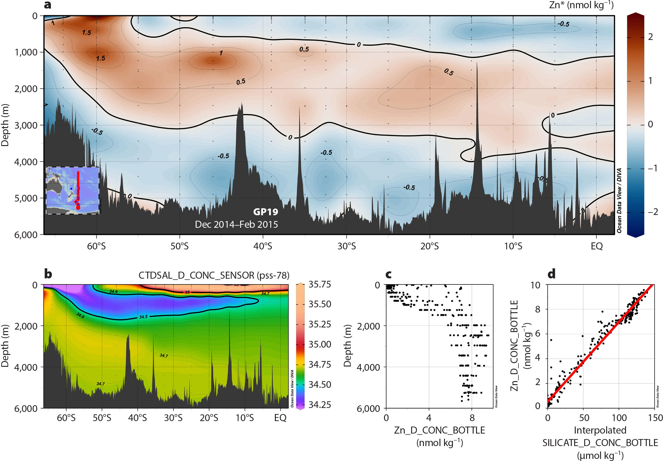
FIGURE 5. Distributions of (a) Zn* and (b) salinity along the GP19 section in the South Pacific. Also shown are (c) profiles of dissolved Zn and (d) correlation of dissolved Zn versus silicate concentration. See the text for details on the calculation of Zn* and interpolated silicate. > High res figure
|
Defining Interpolated Derived Variables
Establish an interpolated derived variable for silicate by choosing View > Derived Variables > Special > Interpolated Variable, then select variable 39 SILICATE_D_CONC_BOTTLE and press Select and Apply.
Establishing Zn Versus Interpolated Silicate Correlation
We now adapt the lower right data window. Right-click on this window and choose X-Variable. Scroll to the end of the list and select Interpolated SILICATE_D_CONC_BOTTLE. Right-click again, choose Y-Variable, and select variable 111, Zn_D_CONC_BOTTLE. Finally, set the Z-Variable to none (first entry). Adapt the X and Y value ranges by first right-clicking and choosing Full Range. Then right-click, choose Set Ranges, and set the minimum value for interpolated silicate to 0. Remove outliers by right-clicking and choosing Sample Filter > Reject Outliers.
Fitting a Straight Line
We now fit a straight line through the interpolated silicate/Zn data points: right-click on the data plot and choose Statistics > Curve Fitting. Leave all settings unchanged and click Construct Curve, keeping notes of slope (0.0644 ± 0.0011) and intercept (0.523 ± 0.082) of the least-squares line. Add the fitted line to the data plot by clicking the Show Curve button.
Expression Derived Variable
We now calculate Zn* by using the least squares line fit obtained above for Zne: Zn* = Zn – 0.0644 * Si – 0.523, where Zn is the measured Zn concentration in nmol/kg and Si is the interpolated silicate in µmol/kg. Expressions like this can be implemented using expression derived variables. Make sure you have already defined interpolated silicate, as described above. Select View > Derived Variables. In the Choices list, click on Expressions, Derivatives, Integrals, then on Expression. In the Labels and Units fields, enter Zn~^* and nmol/kg. In the Input Variables > Choices list, select Zn_D_CONC_BOTTLE (111) and press the << button. Then select Interpolated SILICATE_D_CONC_BOTTLE (at the end of the list) and again press <<. Press the Enter Infix Expression button and enter the expression #1 - 0.0644 * #2 - 0.523, ensuring spaces between all items. Press Convert and then Apply.
Establishing the Zn* Section
We now use the Zn* derived variable as Z variable in the upper large section plot: Right-click on this window, choose Z-Variable, and select the Zn* derived variable at the end of the list. Note that the plotting mode changes to original data points when changing a variable on one of the axes of a data plot. In the following, we will establish gridding using the advanced DIVA tool (Brasseur et al., 1996). Please see chapter 16.6 Gridding Methods in the ODV User’s Guide, https://odv.awi.de/fileadmin/user_upload/odv/misc/odvGuide.pdf, for a better understanding of gridding procedures in general and for guidelines on how to optimally specify crucial gridding parameters. To establish DIVA gridding, right-click on the large section window, choose Properties, and click on the Display Style tab. Click on Gridded field, select DIVA gridding, uncheck Automatic scale lengths, and specify 50 for X and Y scale lengths. Click the General tab and select the crameri_vik color palette. Click Apply. Adjust the Zn* value ranges to [-2.5, 2.5] by right-clicking and choosing Set Ranges. Add contours by right-clicking, choosing Properties, clicking the Contours tab, and clicking the << button. In the Already Defined list, select the 0 contour, under Line select width thin medium, and click << again. Click Apply. Note the systematic Zn* pattern, with positive values mostly associated with low-saline subantarctic mode water in the southern part of the section.
Save your settings to a private view by choosing View > Save View As. A good name would be GP19_Zn-star. As before, you create images of individual data plots or the map by right-clicking on the respective window and choosing Save Plot As or Save Map As.
When using such graphics in your publications or presentations, please be sure to cite the original papers of the data you use. Also cite the IDP2021v2 (GEOTRACES Intermediate Data Product Group, 2023) and the webODV Explore service (Schlitzer and Mieruch-Schnülle, 2021).
Summary
The latest GEOTRACES IDP, IDP2021v2, contains high-quality, intercalibrated global data for more than 500 trace elements and isotopes, covering most of the periodic table. Data value counts are orders of magnitude larger than those available from pre-GEOTRACES times. All ocean basins exhibit good coverage, now allowing detailed mapping of TEIs in the global ocean. Data in the IDPs are associated with easily accessible detailed metadata. IDP data and metadata are distributed in a variety of ways. Here, we demonstrate that detailed data analysis and creation of publication-ready visuals can be done easily using the webODV Explore online service at https://explore.webodv.awi.de. Pre-created section plots and 3D animated scenes can be browsed and downloaded from the eGEOTRACES atlas at https://egeotraces.org. Researchers, teachers, and the interested public are invited to use these resources extensively.
Acknowledgments
We are grateful to the more than 370 researchers worldwide who have released their published or unpublished data to the GEOTRACES IDPs. We also thank the GEOTRACES Data Management Committee, the Standards and Intercalibration Committee, and the Parameter Definition Committee for their fundamental work. Special thanks go to the GEOTRACES International Data Assembly Center (GDAC) at the British Oceanographic Data Centre for carefully collating and delivering all individual data and metadata. Four national data centers prepared GEOTRACES data from individual countries: (a) Biological and Chemical Oceanography Data Management Office (BCO-DMO), (b) Japan Oceanographic Data Center (JODC), (c) LEFE CYBER France, and (d) Netherlands Polar Data Centre (NPDC). The GEOTRACES International Project Office (IPO) maintains the dynamic publication database and coordinated the creation of the GEOTRACES data for oceanic research (DOoR) portal, implemented by experts from the Service de Données de l’Observatoire Midi-Pyrenées (SEDOO). We thank all colleagues for their dedication and professional work. We also thank Roland Koppe, Michael Günster, and Jörg Matthes from the AWI computing center for advice and technical support. Special thanks go to two anonymous reviewers for very carefully checking the step-by-step instructions above and providing valuable comments that helped improve the manuscript. The international GEOTRACES program is possible in part thanks to the support from the US National Science Foundation (Grant OCE-2140395) to the Scientific Committee on Oceanic Research (SCOR).