Purpose

Many undergraduate oceanography students have few opportunities to use ocean technologies on seagoing research vessels. For those who do, understanding sensor function and principles governing instruments like the echosounder systems used to detect the seafloor can be complex and inaccessible. This activity’s goal is to introduce students to the concept and function of underwater acoustics using inexpensive and commercially available sensor building materials. The activity gives students experience with ocean sensors through (1) hands-on engagement with electronics and building of circuits, (2) construction and use of their own simplified echosounder, (3) application of acoustics in ocean bathymetry and seafloor mapping by producing a map of acoustic soundings along a transect, and (4) use of their own data to explore implications of sampling resolution. This activity also serves as an introduction to microcontrollers and environmental sensing, providing students with a foundation for working with additional applications and sensors, and for further exploration.

 

Audience

The activity was designed for an intermediate-level undergraduate oceanography course in ocean technology and engineering. With minimal modifications, this activity is appropriate for introductory through advanced undergraduate-level oceanography courses across a variety of disciplines, as well as for high school marine science, technology, or physics students. Variations of this activity are provided in the supplementary material.

 

Time Required

Prior to conducting this activity, we recommend instructors familiarize themselves with the Sensor Assembly Guide provided in the online supplementary material. Instructors should identify the components of assembly the students will be responsible for and give themselves sufficient time to acquire the necessary materials. We suggest conducting this activity over the course of two lab periods of one to two hours each. During the first session, students review the background information, assemble their sensors, and test the sensors in air. In the second session, students collect and analyze the data. We suggest that students work in small groups of two to four, depending on sensor availability and class size, though this activity can also be done individually.

 

Background

Bathymetry

Bathymetry is the measurement of the depth of a body of water, and bathymetric surveys in which the seafloor is mapped serve many purposes across industries and research fields. For example, depth observations are used to create navigational charts, identify obstructions on the seafloor that could damage fishing gear, investigate underwater archaeological sites, and explore marine geologic phenomena such as underwater ridges and hydrothermal vents. Improving the coverage and resolution of these surveys is critical for maritime industries and for advancing our scientific understanding of many Earth processes.

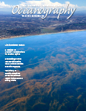
Bathymetric measurements from ships are made using depth soundings. Historically, measurements were made using a weighted rope or wire, referred to as a sounding line, lowered to the seafloor over the side of a ship to measure water depth. The line was marked to indicate standard length intervals and deployed by hand or reel. Once the weight reached the seafloor, the length of line between the mark at the surface and the weight indicated the depth. These measurements were particularly hard to collect in deep water where, even using motorized reels, the process was time-consuming and inefficient for taking multiple measurements. Nonetheless, in the nineteenth and twentieth centuries, sounding machines deploying line or wire via a reel were commonly used for ocean exploration and led to major discoveries of seafloor features such as the Mid-Atlantic Ridge and the Mariana Trench (Dierssen and Theberge, 2014; Figure 1).

 

Figure 1. (a) First recorded bathymetric map of the North Atlantic produced by Matthew Fontaine Maury in 1853 showing an indication of the Mid-Atlantic Ridge (courtesy of the NOAA Photo Library). (b) Modern digital elevation model of the North Atlantic produced using a combination of echosounder and satellite measurements (NOAA National Centers for Environmental Information). > High res figure

 

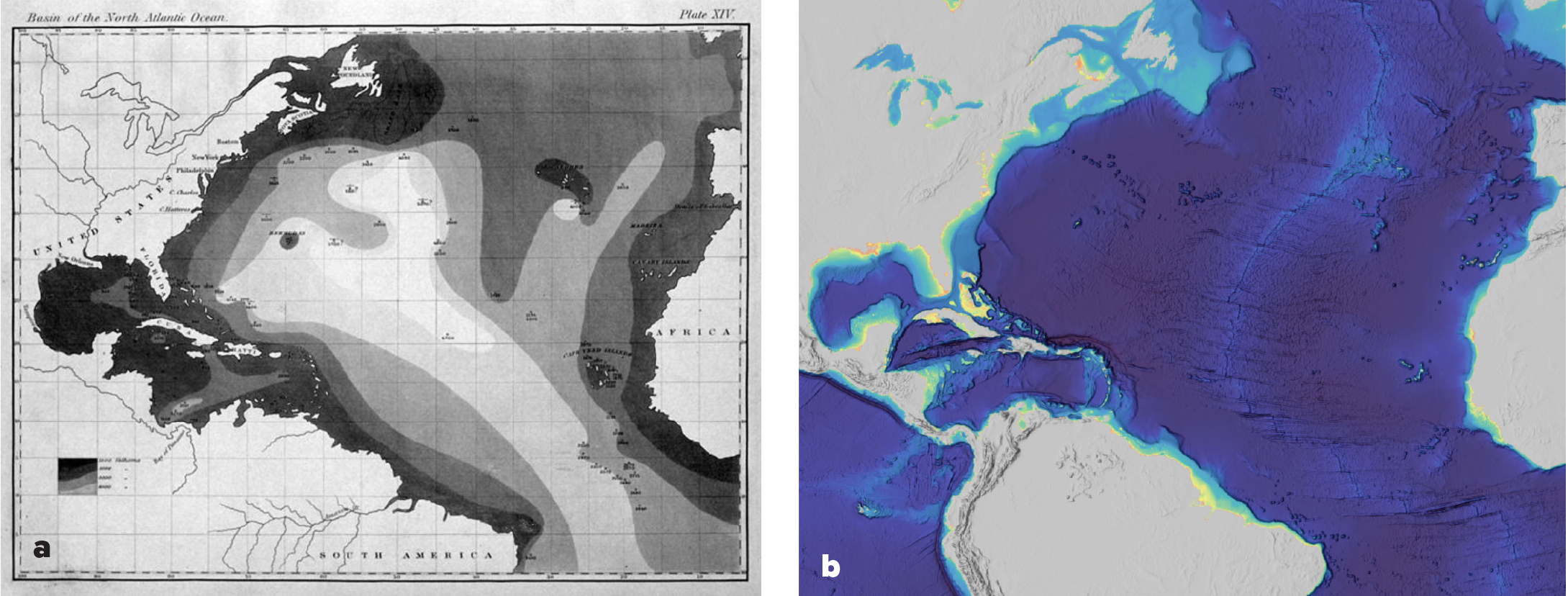
The invention of the piezoelectric transducer in 1917 made it possible for ships to collect echo soundings, depth measurements calculated by transmitting a pulse of sound through the water column and recording the echo that is reflected from the seafloor (Katzir, 2012). In 1922, the US Navy conducted the first seafloor survey using an echosounder and compared depths measured via echo to those measured via sounding line (Anonymous, 1923). The first commercial echosounder systems were produced in 1925 and quickly became the standard depth measurement instrument for hydrographic surveys. With the integration of echosounders into naval and research fleets, our understanding of the seafloor (particularly of deep regions of ocean basins) expanded quickly during the mid-twentieth century. Further technological developments, including multibeam echosounders that image large swaths of the seafloor and satellite-​based ranging, have continued to improve mapping capabilities (Figure 1).

Sound in Water

Sound is a pressure wave, and thus needs a medium to propagate through—a gas, a liquid, or a solid. The speed of sound in water was first measured in 1827 by Colladon and Sturm at Lake Geneva. In their experiment, they simultaneously created a flash of light and rang a bell underwater and measured the timing of the arrival of those signals 16 km across the lake (Colladon, 1893). By measuring the delay between the two signals, they could measure the speed of travel. The speed at which sound travels (c) is a function of compressibility, or its inverse the bulk modulus (B), and density (ρ):

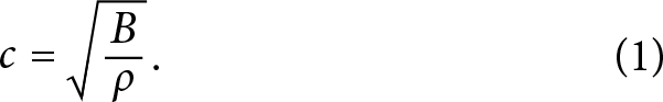
A sound wave is a propagation of a local compression. Mediums with lower compressibility push back with more force for a given decrease in volume when compressed. For example, water has much lower compressibility than air. We can represent a parcel of water as a strong spring and a parcel of air as a weak spring. To compress both springs to the same size, the strong spring (water) requires more force than the weak spring (air). This additional force means that the strong spring will bounce back faster and with greater force to return to its original state. This is the equivalent of a parcel of water exerting the force of a compression wave onto a neighboring parcel. Due to this enhanced transfer of the compressional wave, sound both travels faster and propagates farther in water than in air. Though water is also denser, the difference in density is too small to compensate for the difference in compressibility. Because the speed of sound in any medium is a function of compressibility and density, the speed varies throughout the ocean due to changes in temperature, salinity, and pressure (Wong and Zhu, 1995). On average, the speed of sound in the ocean is approximately 1,480 m s^–1, more than fourfold the average speed of sound in air (344 m s^–1 at sea level and 21°C).

The ability to use sound to detect the seafloor is a function of the intensity of the transmitted signal (I₀), the energy lost during travel, and the reflectivity of the seafloor:

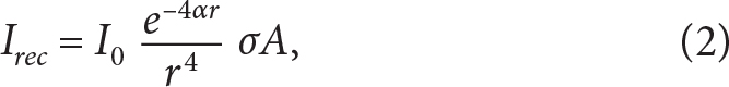
where I_rec is the intensity of the echo received at the transducer, r is the distance between the transducer and the seafloor, α is the absorption coefficient, A is the area of the seafloor the sound reflects off of, and σ is the scattering cross section. The scattering cross section is a function of the acoustic properties of the target (i.e., changes in the sound speed and the density relative to the water) that determines how much energy is reflected (Jackson and Richardson, 2007). Energy lost as the pressure wave moves through the water, represented by  in Equation 2, is a function of both geometric spreading and absorption. Geometric spreading is a decrease in the intensity of the signal per unit area as the signal travels away from the source and the energy spreads out over a larger area. Absorption is the loss of acoustic energy due to the conversion of the signal’s energy to heat.

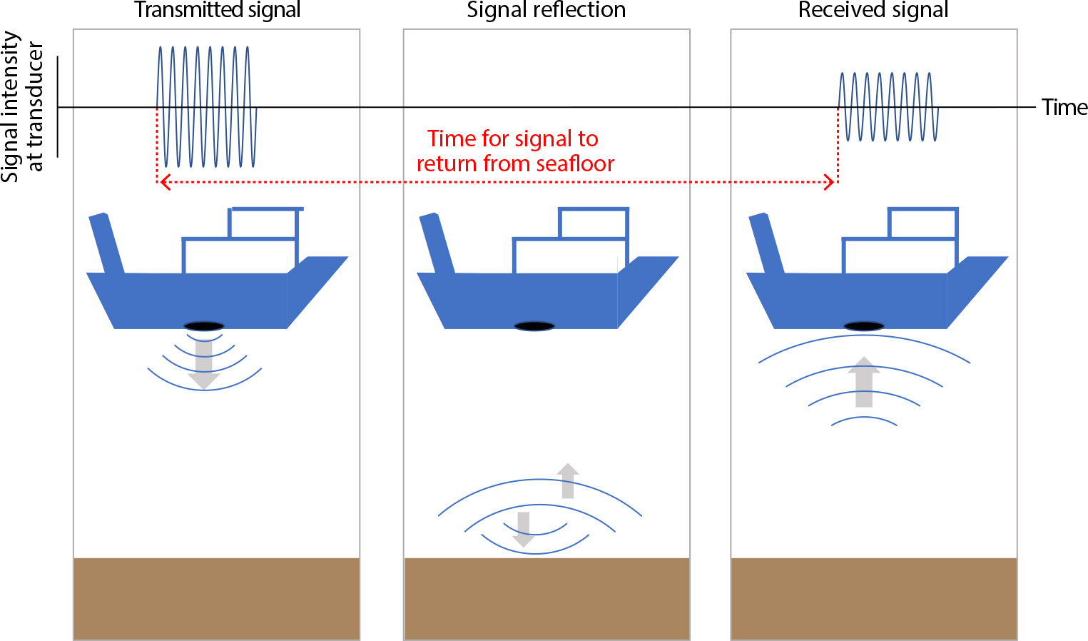
Once an echo from the seafloor is received, the time between when the signal was transmitted from the surface and when the echo was received is used to calculate the distance traveled, and thus the depth (Figure 2):

Here, distance (d) is the product of the speed of sound (c) and the time it takes the signal to travel (t). For example, given an echo with a delay of 0.5 s from the transmitted signal and the speed of sound in water (c = 1,480 m s^–1), Equation 3 tells us that d = (1,480 m s^–1)(0.5 s) = 740 m. The estimated seafloor depth is 370 m, half of the total distance traveled to and from the seafloor by the transmitted signal.

 

Figure 2. Steps of echosounder detection of seabed, with sound wave direction (blue curves) indicated by gray arrows. A signal is transmitted by a transducer at the surface (left box). Upon reaching the seafloor, the signal is reflected to the surface (middle box). The return signal is received by the transducer (right box). The signal intensity is lower upon return due to transmission loss and reflective properties of the seafloor. > High res figure

 

Sampling Resolution

These calculations to (1) detect the seafloor, and (2) calculate the depth based on the distance traveled are the foundations of acoustic bathymetry. The ability to detect, resolve, and map features on the seafloor depends on the sampling resolution and coverage. On many modern vessels, echosounder systems use a single-beam transducer mounted to the hull. For single-beam systems, increasing the horizontal resolution of the bathymetry measurements requires increasing the number of observations of the seafloor collected over a given distance. The distance between measurements is dictated by both the speed at which the ship is moving and the ping rate (number of sound waves transmitted per unit time). In practice, the horizontal resolution is also limited by the angle at which the acoustic beam expands as it moves away from the transducer. The width of the acoustic beam at a given depth is referred to as the beamwidth. The narrower the beamwidth, the smaller the area of the seafloor reflecting the signal. Narrow beamwidths enable collection of more closely spaced measurements. A higher number of independent observations can then be made over a given distance to construct a higher resolution map. More advanced technologies, such as multibeam systems that sample a swath of the seafloor, are elaborations of these same acoustic principles; they increase the sampling resolution by increasing the number and density of seafloor observations that can be measured from a ship’s position.

Active Learning Through Sensor Building

In our activity, students use basic acoustic principles and Equation 3, the distance equation, to repurpose an inexpensive ultrasonic distance sensor as a single-beam echosounder to conduct a bathymetric survey. A key component of this activity is the construction and use of low-cost microcontroller-based sensors that operate using the same principles as commercial instrumentation. Hands-on sensor activities can help students understand the design and use of ocean technology in oceanographic industry and research (Kelley and Grünbaum, 2018). Sensor building exposes students to principles of electronics and engineering, while facilitating an understanding of oceanography and physics concepts through hands-on applications. Through sensor building, students can more effectively learn and apply field-specific concepts (Seroy et al., 2019). Across STEM disciplines, active learning experiences like these have been shown to increase working knowledge of scientific concepts (Freeman et al., 2014) and provide exposure to engineering principles and skills that may benefit students beyond their educational endeavors (Boss and Loftin, 2012).

 

Activity

During this activity, students assemble waterproof ultrasonic distance sensors, and use them to take echo soundings in a local body of water to map bathymetry. These sensors utilize the sonar equation to detect the distance of an object located in the path of the acoustic signal. The associated open-source materials provide an opportunity for a range of engagements with concepts in both oceanography and physics.

Research Question

Students are directed to answer the question: What is the slope and structure of the bottom of a body of water? In the process of collecting data, they will also identify sources of error and assess the precision of their sensors. By collaborating with other students to increase the resolution of their data set, they will also explore the role of sampling frequency in their ability to resolve bottom features.

Materials

To gain experience with sensor technology and demystify sensor function, students should construct their own sensors during an initial class period. Details on microcontrollers, components, and sensor assembly can be found in the Sensor Assembly Guide in the online supplementary material S1 and at PublicSensors (https://www.publicsensors.org/). Sensor components include:

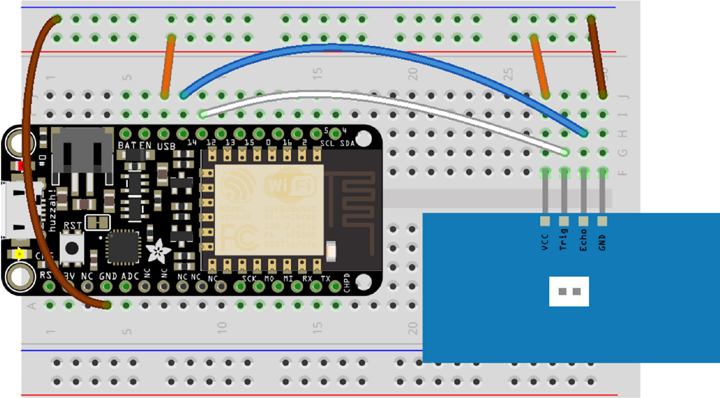
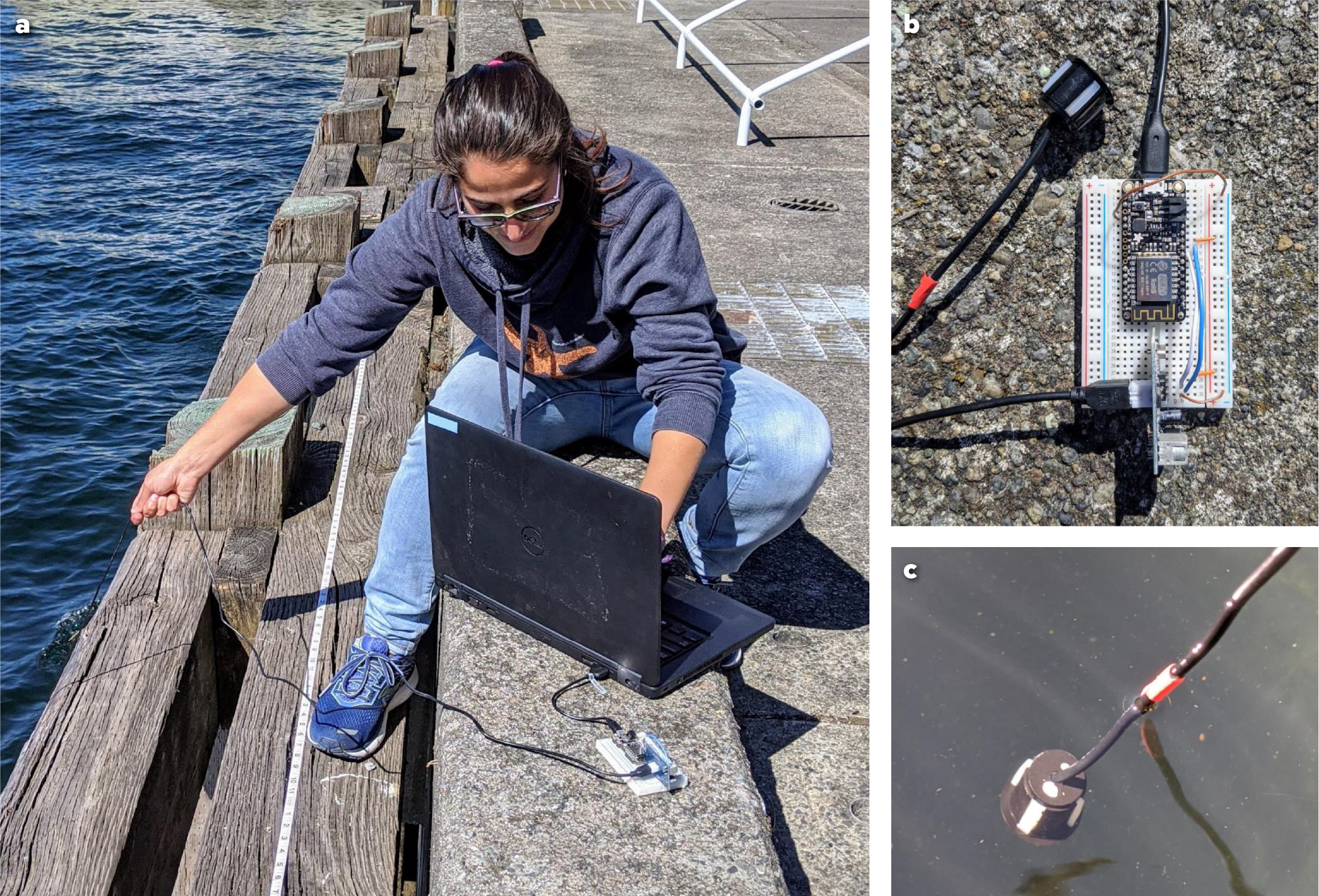
• A MicroPython-based microcontroller. Examples are shown using Adafruit’s Feather HUZZAH with ESP8266 ($17), a MicroPython-based microcontroller (Figures 3 and 4b). Up-to-date firmware and required Python scripts are available on the PublicSensors GitHub repository (https://github.com/publicsensors). Other microcontrollers (e.g., Arduino-based) are compatible, but resources are not provided.
• An ultrasonic distance sensor (hereafter referred to as an acoustic sensor) with a waterproof transducer (JSN-SR04T, $11). This acoustic sensor operates using the same principles as a scientific echosounder. When the sensor receives a trigger signal, it transmits a set of 8 pulses at 40 kHz into the water. The sensor then waits 38 milliseconds for an echo to be received. In water with no obstructions, this timeout corresponds to a theoretical maximum detection distance of ~28 m (~6 m in air). However, loss of signal energy as described in the background can further limit this distance. Due to transducer construction, frequency, and length of transmit signal, the minimum distance an object can be detected in water is ~0.8 m (~0.2 m in air).

Students will also need a laptop for communication with the microcontroller and for data plotting/analysis.

 

Figure 3. Fritzing (https://fritzing.org/) diagram showing the wiring required for the JSN-SR04T using a breadboard. The Trig and Echo pins on the JSN-SR04T should be connected to GPIO 12 and 14, respectively, on the ESP8266 Feather. The GND pin on the JSN-SR04T should be connected to the GND pin on the ESP8266 Feather and the VCC pin on the JSN-SR04T to the USB pin on the ESP8266 Feather. Both the GND and VCC pins can be connected to the microcontroller via the breadboard rails. > High res figure

 

 

Figure 4. (a) Acoustic measurements being taken along a dock. (b) Assembled microcontroller using breadboard connections for acoustic sensor and Feather HUZZAH with ESP8266 microcontroller. (c) The transducer lowered so that the 10 cm tape mark is located at the waterline for consistent sampling. > High res figure

 

Sensor Assembly and Initial Exploration

We recommend providing students with microcontrollers already containing the firmware and necessary files installed, although we encourage instructors to have students conduct as much of the construction and assembly as possible, depending on the time and resources available (see Sensor Assembly Guide sections 3–5 in the online supplementary materials for detailed step-by-step instructions).

Using a breadboard and male/male jumper wires, connect the acoustic sensor to the microcontroller as shown in Figure 3. The transducer cable should be marked with a piece of colored electrical tape or another easily identifiable marker at 10 cm distance from the face of the transducer.

• Connect the microcontroller to a computer with the USB cable. Using a serial terminal (e.g., Beagle Term), connect to the microcontroller. To initialize the sensor, import the hcsr04 library: import hcsr04
• Set pin designations and speed of sound: sensor = hcsr04.HCSR04(trigger_pin = 12, echo_pin = 14, c = 344)
• Use the distance function to collect a measurement (reported in centimeters): sensor.distance()

Students can complete an initial exploration using their sensors in air (c = 344 m s^–1) to assess sensor accuracy and precision, while informing their understanding of potential sources of variability when collecting measurements in water. See Alternative Approaches and Extensions below for optional activities to first determine the speed of sound. Students should collect replicate measurements from a fixed, known distance such as from a tabletop to the floor, wall, or other stationary object. They should consider measurement consistency and possible sources of variability. How are precision and accuracy affected by directly introducing known variability (e.g., measuring the distance from an angled surface or moving a hand between the sensor and the target object)?

Students can assess the role of sampling resolution in resolving features by profiling a feature in air (e.g., a book on the floor) and taking measurements at different spatial intervals relative to feature size. This exploration, analogous to the in-water component of the activity, will help troubleshoot and provide background for understanding how to interpret underwater measurements. Using items on the floor or furniture against a wall, students can take measurements along a continuous transect and consider the necessary number of samples or the interval between measurements that would be required to resolve (1) that a feature is present, and (2) the relief of said feature.

Data Collection

Before students collect their measurements in water, the sampling transect should be defined and students assigned to their sampling positions. We recommend providing students opportunities to test and explore their sensors in water.

• Mark sampling positions at fixed intervals along an accessible shallow body of water (i.e., dock, pool). We recommend approximately 20 sampling locations at one-meter intervals to provide space for groups of students sampling at adjacent positions. However, this is flexible depending on the size and accessibility of the sampling site.
• Assign each group of students a starting point and sampling interval (e.g., Group 1 begins at the zero-meter position and samples every two meters, and Group 2 begins at the one-​meter position and samples every two meters).

Students should collect replicate measurements at each assigned sampling position using c = 1,480 m s^–1. See Alternative Approaches and Extensions below for an optional component to determine the speed of sound in situ. When working in proximity to water, students should take extra caution and be provided with proper safety equipment (e.g., life vests), if necessary.

• At each sampling position, lower the sensor so that the transducer is completely submerged, and the marked 10 cm line is at the water’s surface (Figure 4c).
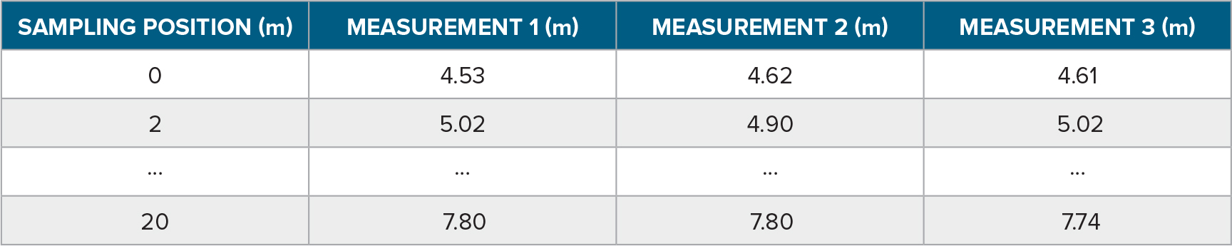
• Collect a measurement of depth and record the value (Table 1). Be sure to include the offset of the distance of the transducer below the water’s surface (e.g., if the sensor reports a distance of 525 cm and the tape mark is at 10 cm, add the additional 10 cm to the distance and record 535 cm).
• Take an additional two measurements at the same position, waiting a minimum of 10 seconds between each measurement.
• Repeat at each subsequent sampling position.

 

Table 1. Example of a data recording table. Students record location as a measure of distance (e.g., “4 m”) as well as values for three measurements collected at that location in units of meters. Additional examples of data recording are included in the supplementary material. > High res figure

 

Data Analysis

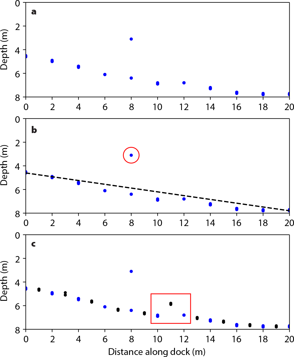
Students should create a bathymetry plot from their own data, where the x-axis is distance along the dock and the y-axis is depth (Figure 5).

• Include all three distances measured at each location to indicate the precision of the depth estimate.
• Groups with alternating starting locations should share their data with each other, to compare the combined data set with their own.

Examples of plotting methods using both Microsoft Excel and Python Jupyter Notebooks are included in the supplementary material. After plotting the data, students should calculate estimates of seafloor depth and slope along the dock, including derived measurements such as height and maximum/minimum relief (angle) of features.

 

Figure 5. Example data analysis figures showing (a) data collected by a single group, (b) the identification of an outlier (red circle) and the slope of the seafloor shown as the dashed line, and (c) combined data sets of two groups, indicating the presence of a feature previously unidentified in the original data set (red box). > High res figure

 

Reflection

Once students have plotted their data, they should consider what their observations imply and the sources of variability. Questions might include the following.

• What features could you identify from your own data?
• Were there features that were possible to discern only in the combined, higher-resolution data set? What were the apparent size and shape of these features?
• How precise was your sensor (how variable were replicate measurements taken at a single location)? What are the possible causes of that variability?
• Identify and remove apparent outliers (https://en.wikipedia.org/wiki/Outlier) from your data set and replot the measurements. Justify your decision for removing these points in the context of the rest of your data. What could have caused measurement outliers? How might this affect the bathymetric profile and statistics?

 

Alternative Approaches and Extensions

• Students can use the sensor to quantify the speed of sound in air or water by calibrating the sensor using an object positioned at a fixed known distance. This can also be accomplished by using a sounding line to ground truth depths at a subset of locations in the same body of water as the bathymetry activity. This is most effective when completed prior to the profiling activity, as an opportunity for students to calculate the speed of sound in one or both mediums themselves. It can be further expanded by conducting the same calibration activity in a variety of mediums with varying densities, such as fresh vs. salt water. Details are outlined in the Activity Extensions supplementary material.
• In addition to taking vertical profiles along a transect, the sensor can be used to take measurements at multiple fixed angles along the original transect. These observations can be used to create a contour plot of bathymetry. Measurements taken at an angle along the transect demonstrate the function of side-scan and multibeam echosounder systems and can be used to investigate more advanced data processing and visualization methods. Students could consider:
  • How does the apparent depth/distance vary as a function of angle?
  • What is the maximum angle at which a return echo is received?

Additional extensions and materials for the approaches described above can be found at PublicSensors (https://www.publicsensors.org/).

 

Additional Online Resources

PublicSensors (http://www.publicsensors.org/)

PublicSensors GitHub Organization (https://github.com/publicsensors)

 

Acknowledgments

We would like to thank the students of OCEAN 351 at the University of Washington who participated in the original iterations of this lab module. We also thank Emmanuel Boss, Tom Weber, and two anonymous reviewers for helpful comments that improved this lab exercise.

Levine, R., S. Seroy, and D. Grünbaum. 2020. Sound and the seafloor: Determining bathymetry using student-built acoustic sensors. Oceanography 33(3):71–77, https://doi.org/10.5670/oceanog.2020.305.

S1: Sensor Assembly Guide (2.2 MB pdf)

S2: Activity Extensions (674 KB pdf)

S3: Student Data Sheet (26 KB Microsoft Excel file)

S4: Bathymetry Lab (7 KB Python Jupyter Notebooks file)

Anonymous. 1923. Echo sounding. The International Hydrographic Review 1.

Boss, E., and J. Loftin. 2012. Spotlight on education—Engineering literacy for undergraduates in marine science: A case for hands on. Oceanography 25(2):219–221, https://doi.org/10.5670/oceanog.2012.61.

Colladon, J.D. 1893. Souvenirs et mémoires: Autobiographie de J. Daniel Colladon. Albert-Schuchardt, Geneva.

Dierssen, H.M., and A.E. Theberge. 2014. Bathymetry: Seafloor mapping history. Pp. 644–648 in Encyclopedia of Natural Resources – Water and Air – Vol II. Yeqiao Wang, ed, CRC Press, Boca Raton, FL.

Freeman, S., S.L. Eddy, M. McDonough, M.K. Smith, N. Okoroafor, H. Jordt, and M.P. Wenderoth. 2014. Active learning increases student performance in science, engineering, and mathematics. Proceedings of the National Academy of Sciences of the United States of America 111(23):8,410–8,415, https://doi.org/​10.1073/pnas.1319030111.

Jackson, D.R., and M.D. Richardson. 2007. High-Frequency Seafloor Acoustics. Springer Science & Business Media, New York, New York, 616 pp.

Katzir, S. 2012. Who knew piezoelectricity? Rutherford and Langevin on submarine detection and the invention of sonar. Notes and Records of the Royal Society 66(2):141–157, https://doi.org/10.1098/rsnr.2011.0049.

Kelley, D.S., and D. Grünbaum. 2018. Seastate: Experiential C-STEM learning through environmental sensor building. Oceanography 31(1):147, https://doi.org/​10.5670/oceanog.2018.123.

Seroy, S.K., H. Zulmuthi, and D. Grünbaum. 2019. Connecting chemistry concepts with environmental context using student-built pH sensors. Journal of Geoscience Education 68(4):334–344, https://doi.org/10.1080/10899995.2019.​1702868.

Wong, G.S., and S.M. Zhu. 1995. Speed of sound in seawater as a function of salinity, temperature, and pressure. The Journal of the Acoustical Society of America 97(3):1,732–1,736, https://doi.org/10.1121/1.413048.

This is an open access article made available under the terms of the Creative Commons Attribution 4.0 International License (https://creativecommons.org/licenses/by/4.0/), which permits use, sharing, adaptation, distribution, and reproduction in any medium or format as long as users cite the materials appropriately, provide a link to the Creative Commons license, and indicate the changes that were made to the original content. Images, animations, videos, or other third-party material used in articles are included in the Creative Commons license unless indicated otherwise in a credit line to the material. If the material is not included in the article’s Creative Commons license, users will need to obtain permission directly from the license holder to reproduce the material.