INTRODUCTION
The deep sea is generally vertically density stratified. No matter how weak the stratification, it is stable. Thus, cross-density (diapycnal) mixing, which results in the upward transport of nutrients and downward transport of heat and oxygen, requires energy, and these transports can only be accomplished by turbulence. Turbulence in the deep sea occurs on spatial scales between 1 m and 1,000 m and on temporal scales between 1 s and 10,000 s, so-called energy-containing turbulent overturning scales. Scientific observational studies of turbulence on such a wide range of scales requires more than one billion simultaneous measurements to resolve all energy-transfer processes at 1 m scales over a 1,000 m range in three directions, as turbulence eventually has a three-dimensional (3D) character. Thus, choices have to be made.
The deep sea is not a stagnant pool of cold water; rather, it is always in motion. Wind and Earth’s rotation are important drivers of water flows. These flows occur not only near the sea surface where stratification is largest due to solar heating but also reach deeper, some even to the deep seafloor. At the large scale, basin-wide circulation occurs with intensified water flows near its boundaries (boundary flows). On medium scales, eddies split off boundary flows. On shorter timescales, tides slosh back and forth and, after interacting with underwater topography, set the stable deep-sea stratification in motion for the generation of internal waves. While internal waves are found everywhere in stratified waters, they freely propagate at frequencies (σ) in the range f ≤ σ ≤ N (e.g., LeBlond and Mysak, 1978). Internal waves at local vertical Earth rotation frequency f are called inertial waves and are, for example, generated after the passage of a storm. The smallest internal waves are at buoyancy frequency N, which is the natural wave oscillation frequency driven by stratification.
Inertial waves provide relatively large vertical water-flow differences (shear) across stratification due to their short vertical scales. Shear deforms stratified layers and thereby generates “shear-induced turbulence,” allowing for diapycnal mixing. In addition to internal waves, any spatially varying water flow can generate shear turbulence, for example, via friction over the seafloor.
Another type of turbulence generation is buoyancy-driven (convection). Warm (and/or fresh) water beneath denser cold (and/or salty) water is statically unstable and generates convection turbulence, as exhibited in ascending and descending plumes (Marshall and Schott, 1999). In the generally stratified ocean, convection rarely reaches from the surface to the seafloor and more often is arrested at the level of matching densities. Examples of convection turbulence generation are nighttime cooling that extends from the surface to several tens of meters depth, and geothermal warming of waters through Earth’s crust that reaches some 100 m above the seafloor.
Here, geothermal heating is understood as the general heat flux from Earth’s mantle that leaks through its crust, other than at underwater volcanic thermal vents. Similar to dense-water formation by surface cooling that leads to convection turbulence, geothermal heating is an effective vertical mixing process. Globally, it contributes about 35 TW of heat flux to the ocean (Davies and Davies, 2010; Wunsch, 2015), an amount about 3,000 times smaller than incoming solar radiation but about 10 times larger than the 3 TW of kinetic energy in tides.
Though commonly observable in geophysics, geothermal heating is very difficult to measure directly in the deep sea outside of hydrothermal vents because temperature differences of less than 0.001°C can only be observed in near-homogeneous waters. Under such conditions, small temperature differences that reflect convection turbulence will not be masked by other oceanographic processes generally associated with larger temperature variations, such as turbulence-suppressing stratification, internal waves and associated turbulence, and passages of (sub-)mesoscale eddies with varying background temperatures.
Because turbulence consumes energy, its production at large scales eventually dissipates at its smallest scales of 0.001 m and 0.01 s, where the mechanical energy is irreversibly converted to heat. Because of a relationship between production, buoyancy flux, and dissipation, turbulence measurements are expressed as the rate of dissipation after certain model assumptions. The turbulence dissipation rate (ε [m2 s–3]) has been mainly inferred from measurements using shipborne one-dimensional (1D) vertical profiling instrumentation. Most used are microstructure profilers, which measure the smallest current-shear variations while sampling at rates of about once per 0.01 s (e.g., Oakey, 1982; Gregg, 1989). Alternatively, CTD profiling is used, which measures the largest turbulent energy-containing overturns as unstable density portions at rates of about once per 0.1 s (Thorpe, 1977).
For time-series analysis of observations at fixed positions, the sizes of large turbulent overturns have been inferred from 1D moored temperature (T) sensors that sampled at 10 m vertical intervals at rates of about once per 100 s (Aucan et al., 2006) and at 1 m intervals at once per 1 s (van Haren and Gostiaux, 2012). Most 1D moored observations have been made in seas that were vertically well stratified in density, so that N > 10f and shear dominates diapycnal vertical turbulent exchange. Three-dimensional measurements needed for understanding full turbulence development are difficult to obtain due to logistical problems, as are (moored) observations from deep convection turbulence areas where dense-water formation occurs.
This paper provides turbulence details observed by high-resolution T sensors moored in a 3D setup above the deep Western Mediterranean seafloor. Box 1 describes the typical physical processes in that region, which mimic many common ocean processes. Variations in turbulence types are presented, ranging from internal wave-dominated, low shear-induced turbulence via moderate convection turbulence from above, to strong convection turbulence from below.
TECHNICAL DETAILS
Instrumentation
Netherlands Institute for Sea Research (NIOZ4) instruments are independent, self-contained high-resolution T sensors with a precision better than 0.0005°C, a noise level of less than 0.0001°C, and a drift of about 0.001°C per month after aging (van Haren, 2018). They are designed to be moored in large numbers on a line in the deep sea to study internal waves and turbulence types. The instruments also house tilt and compass sensors to monitor undesired motions of the mooring line dragged by large-scale water flow. Every four hours, the internal clocks of all sensors on a mooring are synchronized, so that sampling times are less than 0.02 s off. T sensors sample at a rate of once per 2 s. With such high-resolution sensors, turbulence types can potentially be observed in the weakly stratified deep sea, but only under particular conditions, after considerable post-processing corrections, and when the sensors are located in a densely instrumented, moored array. Here, T sensors are used in a five-line (5-L), 3D mooring to collect information on the transition between stratification-hampered 2D (anisotropic) and full 3D (isotropic) turbulence.
The 5-L is a 6 m tall, 3 m diameter, fold-up, high-grade aluminum structure (van Haren et al., 2016). It consists of two frames each 1.7 × 1.7 m that support a set of four arms or extensions (Figure 1b,c). T sensors are taped to five 105 m long, 0.0063 m diameter nylon-coated steel cables that extend from the upper to the lower frame. Four of the instrumented lines (lines 1–4) connect the corner tips of the upper and lower frame arms; the fifth instrumented line, “line c,” connects the centers of the upper and lower frames (Figure 1d). Corner lines are horizontally separated by 4.0 m from line c and are located 5.6 (or 8) m from each other. During deployment, the four arms are extended after the mooring is lifted overboard (Figure 1c,d). The 3D 5-L mooring then free falls to the seafloor in a manner similar to the setting of a 1D oceanographic mooring. Corner and center line weights supply tension of more than 1 kN per line, and top flotation attached with a single line above 5-L provides at least 5 kN total net buoyancy once the mooring reaches the seafloor.
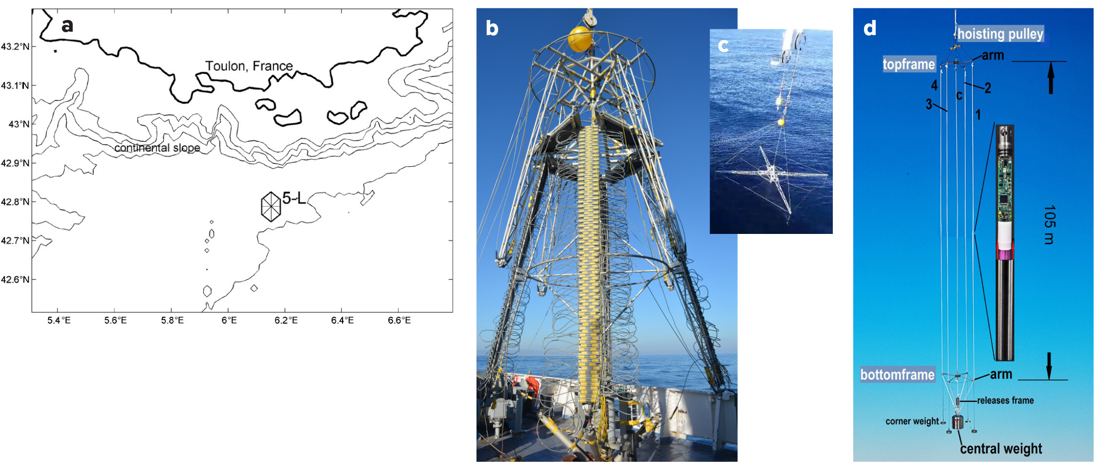
FIGURE 1. Five line (5-L) mooring frame and deployment site. (a) Location of 5-L (star) about 40 km south of Toulon, France, and 12 km south of the continental slope. Depth contours are drawn every 500 m. (b) 5-L folded up and ready for deployment onboard R/V L’Atalante. (c) 5-L unfolded overboard, just before release to free fall. (d) Model of completely extended 5-L to scale, except for the T sensor on the right. > High res figure
|
A total of 340 NIOZ4 T sensors were used in this study. One hundred four T sensors were attached at 1.0 m intervals to line c, with the lowest sensor at 5 m above the seafloor at z = –2,475 m. Fifty-three T sensors were attached at 2.0 m intervals to lines 1–4, and four T sensors were attached at 1.0 m intervals to each 25 kg corner-line weight so that the lowest sensor was 0.5 m above the seafloor. Above 5-L at z = –2,310 m, a single point 2 MHz Nortek AquaDopp acoustic current meter sampled water flow every 150 s.
The mooring was deployed at z = –2,480 m, about 40 km south of Toulon harbor (Figure 1a) for 10 months between November 2017 and September 2018. The local bottom slope is nearly flat, <1° from horizontal, and featureless, though the mooring was only 12 km seaward of the foot of the steep continental slope.
For calibration purposes and to establish the local temperature-density relationship, shipborne CTD profiles were obtained within 1 km of the 5-L site during the deployment and recovery cruises. During another cruise in 2020, a CTD profile was obtained 6 km northeast of the 5-L site.
Moored Instrument Performance
The T sensors performed well, but only for the first 4.5 months following deployment. Bad batteries caused 50% failure around day 460 and more after that. Less than 10% of the T sensors collected data during the 10 months underwater. Detailed analysis thus focuses on data collected before day 450, when fewer than 49 (15%) of the T sensors were either not working, showed calibration problems, or were too noisy. Data are interpolated between neighboring sensors. The current meter worked fine for the entire 10 months underwater.
Post-Processing of Moored T Sensor Data
After calibration, T sensor data were corrected for pressure and compressibility effects by transferring them to Conservative Temperature Θ (IOC et al., 2010). To correct for instrument drift so that our results would not include unrealistic unstable conditions, portions of the T sensor data were sought in which dΘ/dz = 0 < 0.00001°C/100 m over the entire range of observations as in homogeneous waters. Existence of such homogeneous waters in the deep Western Mediterranean was established using previous extensive CTD observations, especially in the central and southern parts of the basin. These data extend up to about 800 m from the seafloor (e.g., van Haren et al., 2014), covering two-thirds of the vertical range of 1,200 m for geothermal heating dominance suggested by Ferron et al. (2017). Closer to the continental slope at the 5-L site, <200 m of vertically homogeneous layers were expected due to larger submesoscale activity resulting in ascending and descending water masses and associated weak stratification.
RESULTS
Monitoring the Mooring Deployment
The eight T sensors on the frame arms monitored the deployment of 5-L, including the sinking and the final positioning on the seafloor under flotation tension (Figure 2). During the free fall, the initial vertical speed was just above 1 m s–1 and decreased to about 0.7 m s–1 due to flow drag during the remainder of the fall (Figure 2a). The water temperature (Figure 2b) decreased with time, as expected for a stable environment, and subsequently increased with time, due to slight compressibility effects in the weakly stratified waters for pressures p > 1.5 × 10⁷ Pa (Figure 2a). After the mooring reached the seafloor, temperature varied by ±0.0001°C (Figure 2b), which indicates near-homogeneous waters, close to instrument noise levels. The mooring’s aluminum frame was sturdy and virtually stable, with the two square frames aligned to within 1° (Figure 2c) under drag of 0.1 m s–1 water-flow speeds. During the 10-month deployment, the mooring remained almost unaffected by water-flow drag, even when bottom currents increased to 0.35 m s–1 in late winter; it rotated no more than ±3° under maximum cable and frame vibrations of 10 s–1 and 2 s–1, respectively.
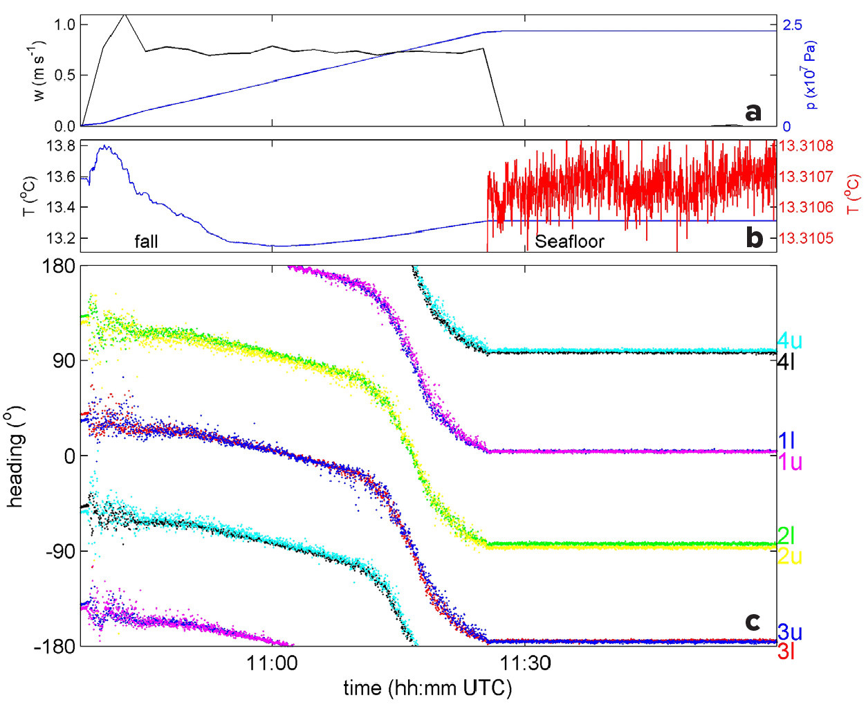
FIGURE 2. Operational observations during deployment of 5-L, from the free-fall descent to a stationary position at the seafloor. (a) Vertical velocity (black, with scale at left; positive is when the mooring descends) and pressure (blue, with scale at right) registered every 150 s by the current meter 170 m above the central weight. (b) Temperature (blue, with scale at left) and its 2,000 times magnification arbitrarily shifted vertically (red, with scale at right). (c) Compass headings of all eight mooring-frame corner sensors on upper (u) and lower (l) aluminum frames. > High res figure
|
CTD Profiles
Similar variations are seen in Θ among the three CTD profiles (Figure 3a), as well as in density anomaly σ2 referenced to 2 × 10⁷ Pa (Figure 3b). The vertical density stratification, which corresponds to –dσ2/dz ~ N2, declines in value from the surface toward the seafloor (Figure 3c). At 200 m above the seafloor, stratification is very weak, as N calculated from CTD data varies between 0 and 2f, with a general mean value of about N = 1f = 1.36 cycles per day (cpd). N is computed over dz = 100 m vertical scales. In the same vertical range, maxima of small-scale buoyancy frequency Ns, computed over dz = 1 m, are observed up to about Ns,max = 4f (Figure 1c). The vertical range of N = 0 (homogeneous, no stratification) extends less than 100 m from the seafloor in these profiles, confirming the suggested influence of the nearby continental slope and its stratified boundary flow, which suppress the formation of hundreds of meters of large homogeneous layers such as found in the central Western Mediterranean (van Haren et al., 2014). Knowledge of the weak stratification is thus important for studies of internal wave dynamics. Such knowledge can only be achieved via careful post-processing of moored T sensor data.
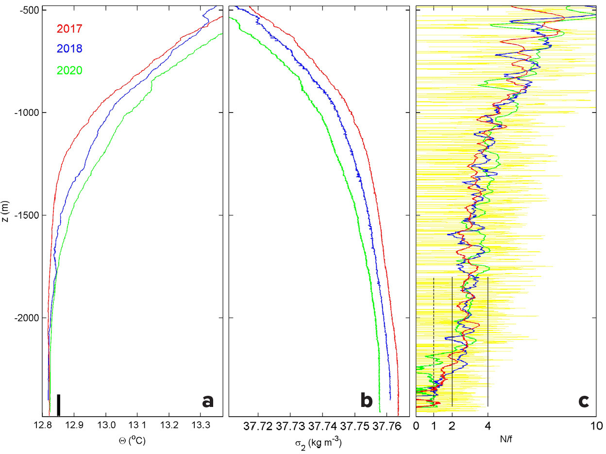
FIGURE 3. Lower 2,000 m of shipborne CTD profiles obtained near 5-L site during cruises for deployment (red, with lowest value 5 m above the local seafloor) and recovery (blue, with lowest value 80 m above the seafloor due to winch constraints), with an extra profile from October 2020 (green, with lowest value 0.5 m above the seafloor). (a) Conservative Temperature. The vertical bar indicates the range of the moored T sensors. (b) Density anomaly referenced to 2 × 10⁷ Pa. (c) Buoyancy (N) to local inertial (f) frequency ratio smoothed over 5 × 10⁵ Pa (and in yellow over 6 × 10⁴ Pa for CTD2020, which represents Ns). > High res figure
|
Given the relatively tight and consistent Θ-σ2 relationship (Equation S1 in the online Supplementary Materials) evident in shipborne CTD data, the moored T sensor data can be used to infer turbulence dissipation rates (Equation S2). Mean turbulence values are calculated by arithmetically averaging ε(t, z) in the vertical […] or in time <…>, or both. Although Θ data are analyzed throughout, “temperature” is used henceforth as a shorthand for Conservative Temperature.
Environmental Variability with Time and Frequency
Flow speeds measured at z = –2,310 m were typically <0.1 m s–1 between late summer and early winter but doubled periodically, with peaks of 0.35 m s–1 due to increased eddy activity in late winter and spring (Figure 4a). A single 10-month record of temperature varied by <0.01°C, with most of the variation occurring in a limited number of positive (warm-water) peaks between days 430 (early March) and 560 (mid-July). One-third of the temperature variation was attributable to instrumental drift that caused a low-frequency nonlinear increase with time, mainly during the first month (Figure 4b).
The positive peaks in vertical temperature difference ΔΘ stand out and reflect stable stratification, not only over 98 m but also over 16 m vertically near the seafloor (Figure 4c), and they align with warm-water peaks (Figure 4b). The positive ΔΘ implies very small homogeneous layers above the seafloor, which are generally <100 m vertically and occasionally <16 m during spring.
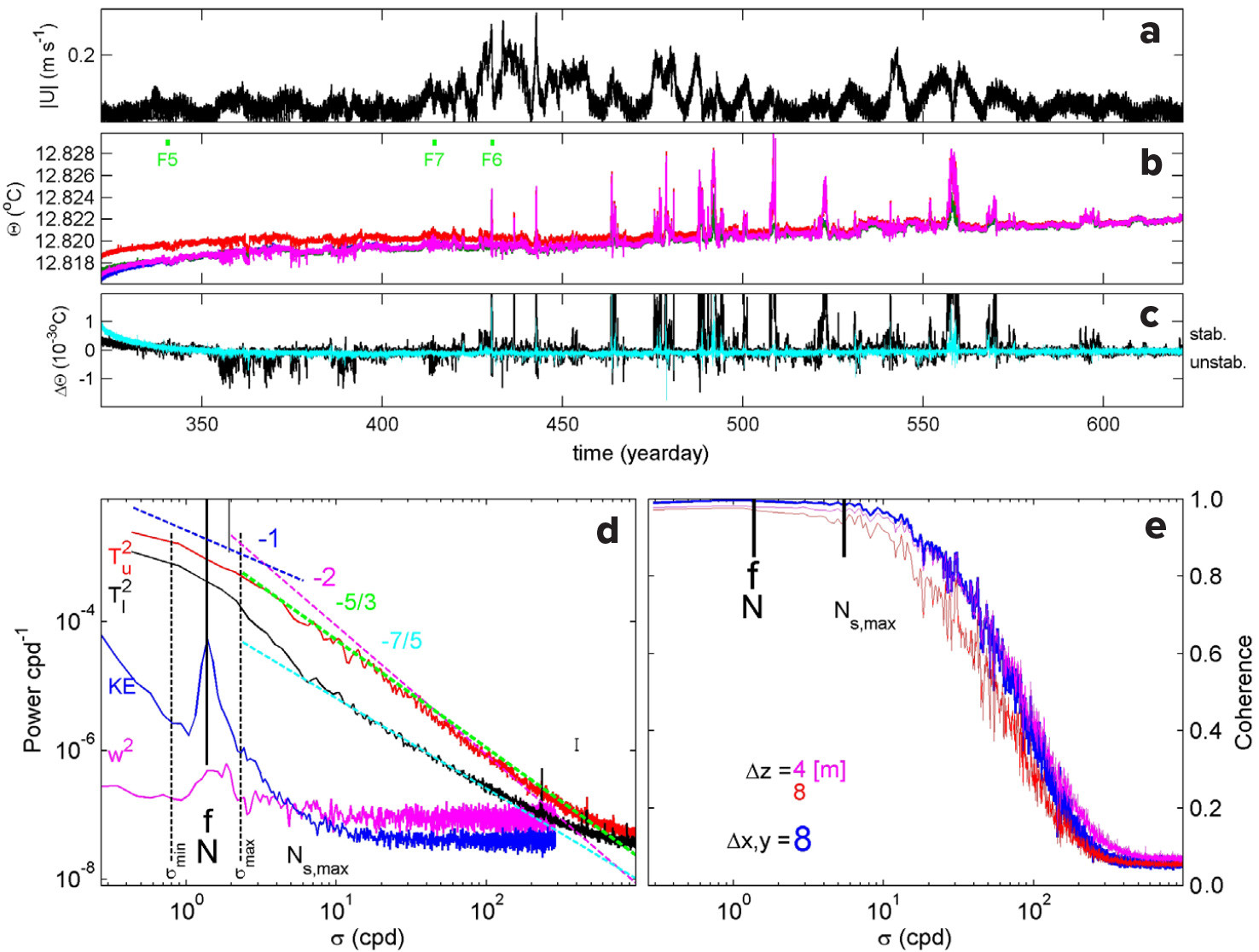
FIGURE 4. Overview of 10 months of mooring data. (a) Horizontal water-flow amplitude observed by the current meter at z = –2,310 m. (b) Calibrated, but not drift-corrected, Conservative Temperature from –2,475 m (blue), –2,459 m (green, barely visible), –2,393 m (red), and –2,377 m (purple) of line 1. Green ticks indicate days of F(igures) 5–7. (c) Difference between records from panel (b): from –2,459 minus –2,475 m (16 m difference, light blue) and –2,377 minus –2,475 m (98 m difference, black). Data are low-pass filtered with cut-off at 1,000 cycles per day (cpd). (d) Moderately smoothed power spectra for temperature between days 322 and 425 in panel (b), and averages for the lower two T sensors (black) and the upper two (red). Current meter data provide arbitrarily vertically shifted spectra of horizontal kinetic energy (KE) and vertical current variance (w2). The small vertical line indicates the semidiurnal lunar tidal frequency, and the long vertical dashed lines indicate the internal wave band for weak stratification N = f. Ns,max = 4f denotes the average of maximum small 2 m-scale buoyancy frequencies per profile. Several spectral slopes are given in the log-log plot with, for example, –1 indicating σ–1 (see text). (e) Coherence spectra between all possible pairs of T sensors across indicated vertical and horizontal distances, averages for days 322 to 425. The 95% significance level is at coherence = 0.05 so that values extend above noise for σ < 200 cpd. > High res figure
|
Both ΔΘ records also show significant negative values that reflect unstable conditions (Figure 4c). Largest negative ΔΘ are observed in early winter (between days 350 and 400), well before positive peaks occur. For Θ-σ2 relationship (Equation S1), negative ΔΘ indicates rather persistent large-scale instabilities, possibly related to convection. For example, observed ΔΘ = –0.001°C over 98 m and stable N = 2f higher up translate to a net vertical homogeneous range of 250 m from the seafloor, well exceeding the 105 m range of the moored T sensors. These inferred near-homogeneous layers above the seafloor are the largest in the 10-month record.
The spectral overview (Figure 4d) for the first 3.5 months of T sensor data demonstrates that the kinetic energy of local horizontal water flows is dominated by a peak at f (about 17.5-hour periodicity) and larger energy at sub-f (about 10-day periodicity). The vertical water-flow component shows a small but significant peak bulge in variance around f, confirming rotation-driven internal waves in very weakly stratified waters. It includes a small semidiurnal tidal peak.
The mean T-variance spectra do not show significant peaks but rather several slopes that vary with frequency band and vertical position. Within the internal wave band [σmin,σmax] = [0.6f, 1.7N] in weak stratification N = f, spectral slopes for both upper and lower sensor data scale with σ–1, as observed in the open ocean (van Haren and Gostiaux, 2009). The extension of the internal wave band to frequencies σ < f and σ > N (for equations, see LeBlond and Mysak, 1978) is related to waves driven by Earth’s rotation that manifest themselves in weak stratification.
For the upper sensors at σmax < σ < 300 cpd, the slope scales approximately with σ–5/3, reflecting the inertial subrange of (shear-induced) turbulence for a passive scalar (Tennekes and Lumley, 1972; Warhaft, 2000), before rolling off to noise levels. Although this range includes Ns, the range N < Ns < Ns,max describing internal waves in small stratified layers, the slope does not reflect freely propagating internal waves that scale with σ–2 (Garrett and Munk, 1972).
For the lower sensors, the T variance is about one order of magnitude lower compared with the upper sensors. For σmax < σ < Ns,max, the slope scales with σ–2.5, representing either internal waves or, more likely, finestructure contamination (Phillips, 1971). For Ns,max < σ < 120 cpd, the slope scales with σ–7/5, which reflects an active scalar (Bolgiano, 1959; Pawar and Arakeri, 2016) and convection turbulence.
Thus, spectrally, T sensors show a limited internal wave band related to the weak stratification N = 1f throughout the vertical range of observations. At frequencies higher than the internal wave band, extended finestructure and mainly shear-induced turbulence are observed away from the seafloor. In contrast, at these frequencies, mainly convection turbulence is observed near the seafloor.
In terms of small-scale comparison between all independent pairs of T sensors, strong coherence is found up to Ns,max, before rolling off to noise values (Figure 4e). The 8 m horizontal scale matches that of the 4 m (and even smaller) vertical scale, suggesting vertically restricted anisotropic turbulence. For about 150 < σ < 300 cpd, the 8 m horizontal scale coherence matches that of the 8 m vertical scale coherence, which suggests isotropic turbulence with motions unrestricted in all directions. In the range Ns,max < σ < 150 cpd in between, convection turbulence observed at the lower T sensors marks the transition from anisotropic “stratified” to isotropic turbulence.
DYNAMICS DETAILS
Moored T sensor data highlight three types of dynamical stability features near the seafloor close to the continental slope of the deep Western Mediterranean: (1) mainly stable stratification, deep internal waves, and some turbulence; (2) mainly apparently stable stratification and considerable turbulent bursts; and (3) mainly apparently unstable stratification and large turbulence.
Mainly Stable Stratification, Deep Internal Waves, and Some Turbulence
In summer and autumn, between about days 210 and 340, the waters near the mooring site are weakly but stably stratified, and double-inertial period internal waves appear close to the seafloor (Figure 5a). Turbulence activity is as low as in open-ocean interior waters (Figure 5b), with one-day, 105 m mean [<ε>] = 2 ± 1 × 10⁻¹⁰ m2 s–3 for [<N>] = 2.0 ± 0.2 × 10⁻⁴ s–1 ≈ 2f. Nevertheless, waters are not quiescent as they are in laminar flows, and bursts of turbulence occasionally appear (e.g., on day 340.3, Figure 5b). No convection turbulence is observed from the seafloor upward. The stable vertical density stratification apparently masks any direct observation of geothermal heating.
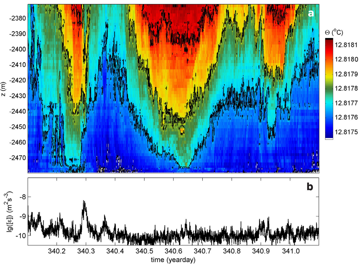
FIGURE 5. Example of one-day detailed T sensor corner line 1 observations of apparent stable stratification and deep internal waves in late autumn. (a) Time-vertical image of Conservative Temperature. Black contours are drawn every 0.0002°C. The total temperature range is 0.0007°C. The seafloor is at the x-axis, so that the lowest T sensor is at 0.5 m above it. (b) Time series of logarithm of vertically averaged turbulence dissipation rate calculated from the data in panel (a). > High res figure
|
Mainly Apparently Stable Stratification and Considerable Turbulent Bursts
The stable N = 2f stratification is built up in spring, between about late-winter day 65 (430 in the following year) and mid-summer day 210 (575). During this period, deep-water flows reach speeds of >0.1 m s–1, up to 0.35 m s–1 (Figure 4a). Such flows are occasionally, but not always, accompanied by positive peaks in temperature (Figure 4b).
The Θ peaks reflect warm waters either coming from above, possibly via convection, or via internal waves that push the stable stratification downward. Figure 6 shows details of part of such a Θ peak, where the warmest core is to the right of the image. The water flows steadily at 0.25 m s–1 from the north-northwest during this period. The flow is probably related to a meandering boundary current or eddying and, in this example, may advect the warmer plume that was generated nearer the coast. The time period coincides with that of potential dense-water formation near the surface, which can reach several hundreds of meters deep every year and extend to the seafloor once every two to five years (Mertens and Schott, 1998; Somot et al., 2018). The local stable stratification peaks to N ≈ 4f, but quasi-convection turbulence (from above) is obvious with ascending and descending cold- and warm-water plumes.
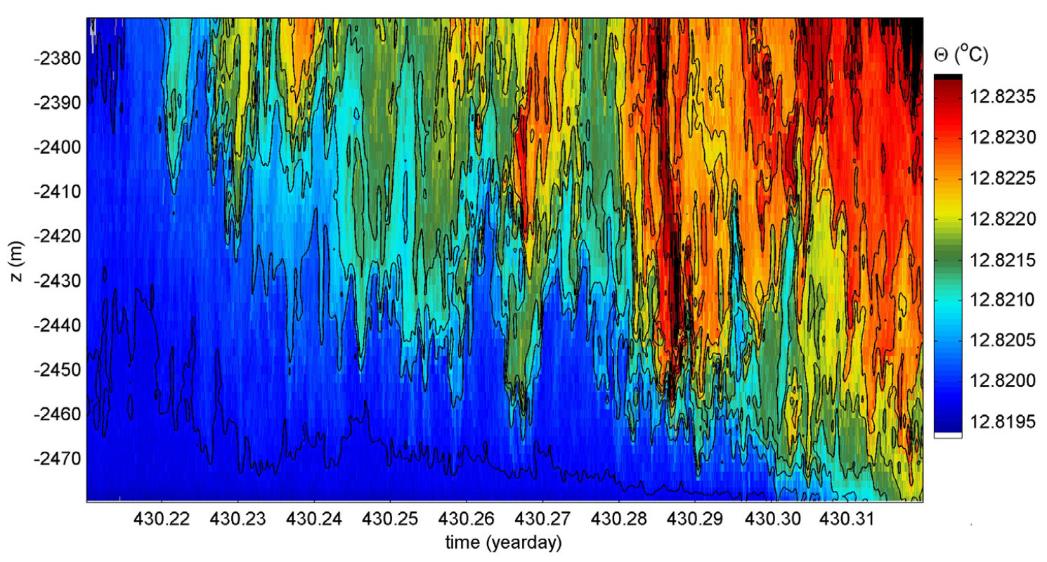
FIGURE 6. Same as Figure 5a, but for 104 s (0.11 day) of observations of apparent stable stratification and convection plumes from above in late winter, and with different color scale, which covers a temperature range of 0.0045°C. > High res figure
|
Convection beneath stable stratification has been attributed to internal waves and active turbulence that overcome the local reduced gravity (gravity times the relative density difference) in the lower 50 m above the floor of Lake Garda, where mean N = 2f (van Haren and Dijkstra, 2021). In that 340 m deep alpine lake, convection turbulence initiated by internal waves was observed below strongly stratified waters. Downward internal wave motions accelerate convection turbulence in the near-homogeneous layer below. These accelerations overcome the reduced gravity of the weak stratification at timescales of the minimum buoyancy period, or largest turbulence timescales. Figure 6 mimics unstable convection turbulence simulations influenced by rotation (Bofetta et al., 2016).
For the present data, it is not possible to rule out the partial density-compensation effects of salinity in different water masses (from above), which may cause ambiguous temperature-density relationships due to dense-water formation in late winter and spring. Adopting a conservative stand because of the possible ambiguity in the sign of the temperature-density relationship, no turbulence values are given for this period. (If turbulence values are calculated using Equation S2, they fall between those of subsections above and below.) Warm-water blobs coming from above are surrounded by unstable waters >105 m above the seafloor (see the leftmost part of Figure 6). Note that the entire temperature range of this figure is about 0.0045°C and that convection detection generally requires a smaller range.
Mainly Apparently Unstable Stratification and Large Turbulence
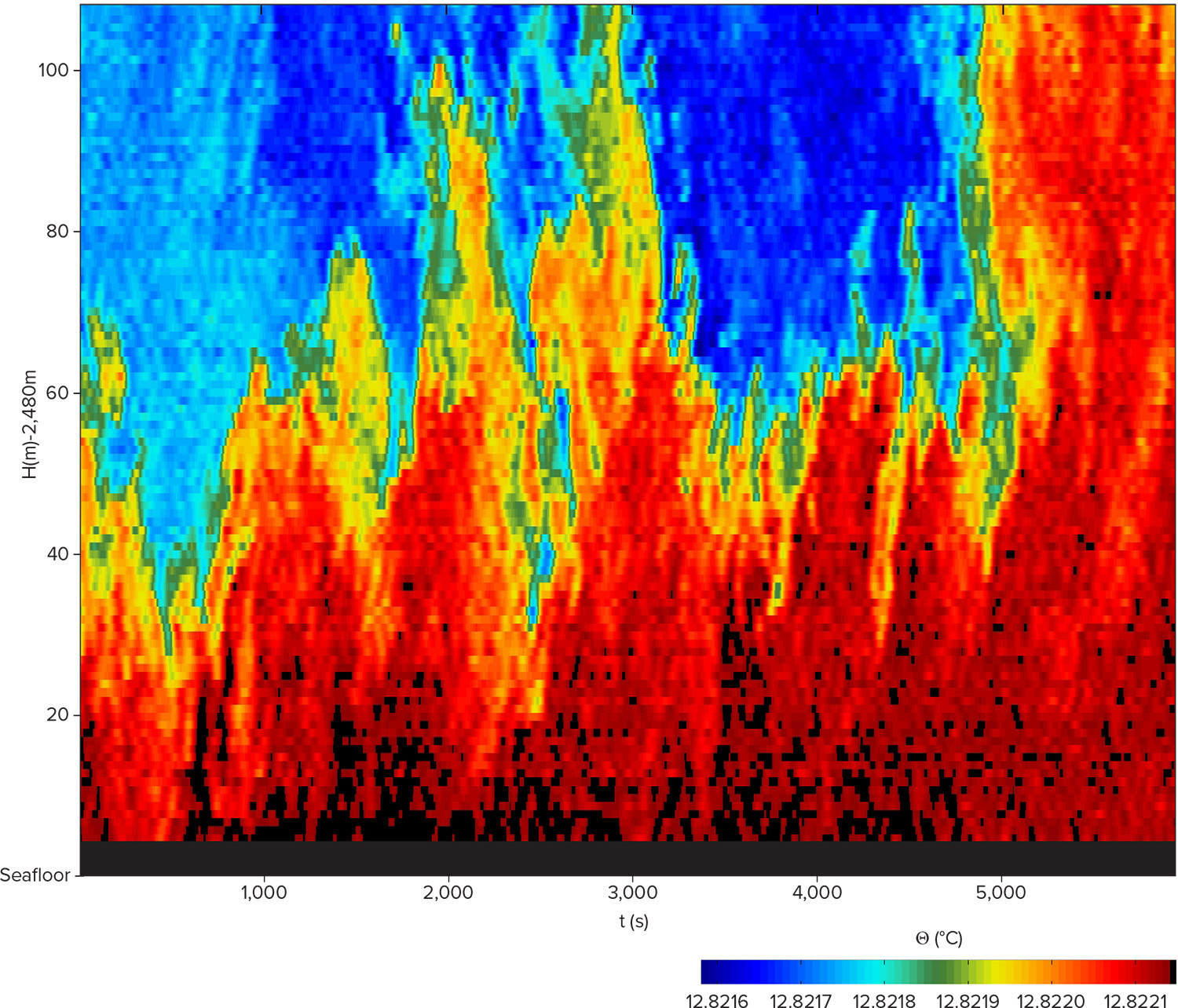
In winter between days 340 and 430, waters near the seafloor are sufficiently weakly stratified so that presumed geothermal heating may be directly observable (Figure 7). During this period, deep dense-water formation is not yet active, as near-surface waters are not sufficiently cooled and evaporated to become denser than all underlying waters (e.g., Mertens and Schott, 1998). Thus, convection from above that may mask geothermal convection from below is not expected before the end of winter, if it occurs at all, and is not blocked by stratified boundary flow. However, stratification higher up arrests the eroding geothermal convection just as stratification confines convection due to nighttime cooling near the sea surface.
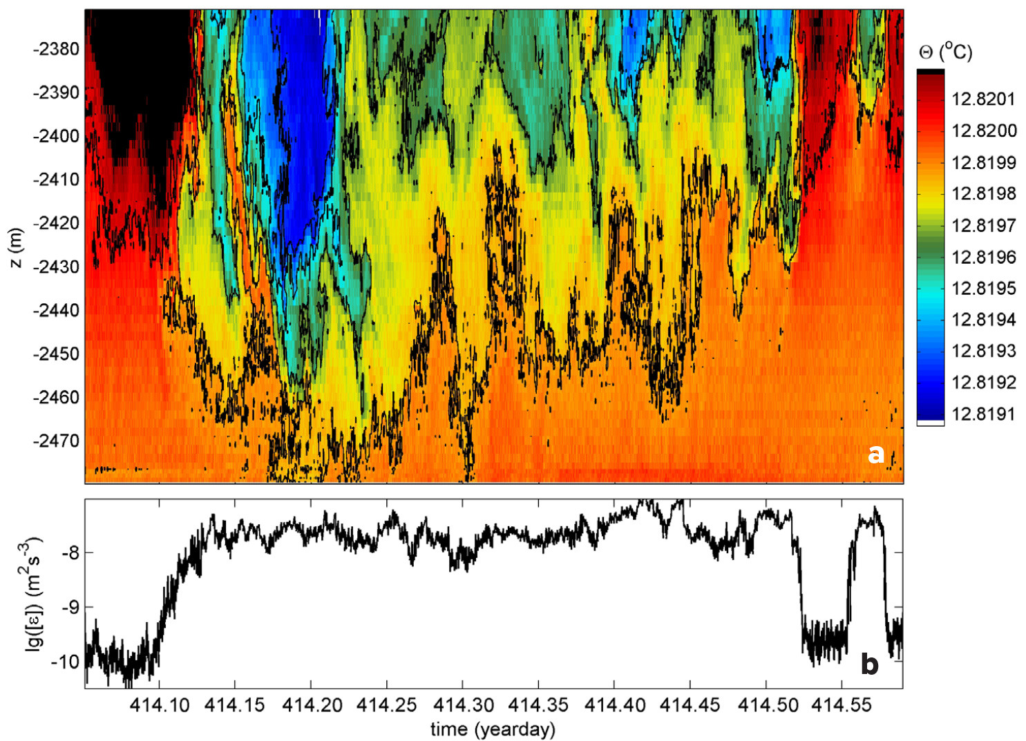
FIGURE 7. Same as Figure 5, but for 0.54 day of observations, including 0.38-day (half inertial period) instability and apparent convection from below, geothermal heating, and relatively warm stratified convection from above on the sides in winter. Compared to Figure 5a, a different color scale is used in panel (a), which covers a temperature range of 0.0011°C. > High res figure
|
The 0.0011°C temperature range in Figure 7a shows warmest waters near the seafloor for half an inertial period (0.38 d), with typical “plumes” of alternating (ascending) warm and (descending) cooler waters depicting natural convection turbulence. The individual plumes are variable in temporal and vertical extent as well as intensity. They resemble the irregular plumes of opposite signs in Figure 6. In Figure 7, the warmer waters near the seafloor heat waters above. This heating varies with time, as temperature is not constant near the seafloor. The convection from below is surrounded and capped by stably stratified waters. Using conventional Thorpe-scale analysis (Equation S2), as has been satisfactorily applied for sea surface convection turbulence eroding stratified waters below (Kumar, 2021), the 0.54-day, 105 m mean [<ε>] = 2.2 ± 1.5 × 10⁻⁸ m2 s–3 for [<N>] = 2.0 ± 0.2 × 10⁻⁴ s–1 ≈ 2f.
Recall that the mean buoyancy frequency is determined from the reordered, stably stratified vertical profiles. Its value is the same as the general value for the stable periods to within error. This suggests that convection turbulence is working on the same stratification as shear-induced turbulence might have.
Averaging data from Figure 7 only over the period of convection, the 0.38-day, 105 m mean [<ε>] = 2.8 ± 1.6 × 10⁻⁸ m2 s–3 for above [<N>]. The variation with time is considerable in ascending and descending motions, but only about one order of magnitude in vertically averaged dissipation rate. Integrated over the 105 m range of observations, however, the turbulence energy dissipation rate equals 3 mW m–2 after conversion with density of seawater. This value is just 3% of the average amount of the vertical flux attributed to geothermal heating in the area, which is 100 ± 30 mW m–2 (Pasquale et al., 1996). Even if considering a turbulent mixing efficiency (proportion of kinetic energy consumed by mixing) of about 0.5, which is typical for vertical natural convection (Dalziel et al., 2008; Gayen et al., 2013; Ng et al., 2016), the calculated dissipation rates here fall short by one order of magnitude of a presumed value of 50 mW. Two suggestions are given for the apparent discrepancy in Box 2.
DISCUSSION AND CONCLUSIONS
The high-resolution observations collected by moored T sensors revealed turbulence and internal wave processes in very weakly stratified waters of the deep Western Mediterranean. These observations confirm the importance of geothermal heating to turbulent mixing of deep-sea waters, although not to the 1,200 m vertical extent calculated by Ferron et al. (2017) for the central Western Mediterranean. Although geothermal heating induced the greatest turbulence, it was only observed in winter. At other times, convection turbulence induced by geothermal heating was masked by other processes such as stratification, which dampens turbulence, and convection from above. While no information is available on the period of the year when Ferron et al.’s (2017) shipborne microstructure profiles were obtained, their deep Ligurian Sea values near the continental slope were 1–3 × 10⁻⁹ m2 s–3, which falls between the low and high values presented here. The moored T sensor data collected near the deep seafloor show that variations in temperature affect the strength and the types of turbulence. These variations in turbulence strength and type are summarized below.
Throughout spring, convection turbulence from below induced by geothermal heating alternates in time with convection turbulence induced by apparently stable warmer waters from above. Downward advection of such warmer waters by convection processes near the surface and/or by (sub)mesoscale eddies also occurs with inertial and semi-inertial periodicities. Deep-water flow speeds regularly double in size compared to winter, and these stronger flows may advect the stable warmer waters horizontally over the mooring site and occasionally resuspend sediment, which will be transported upward by the convection turbulence.
By early summer, turbulence becomes weaker in time and smaller in amplitude, presumably dampened by added heat and increased stratification from above.
In late summer and autumn, convection turbulence is weak, from both below and above. The stratification of typically N = 2f extends nearly to the seafloor, dampens vertical turbulent exchange, and supports internal waves of considerable amplitudes (>10 m). While these internal waves provide internal shear, their friction effects over a flat seafloor are generally small. Gradually, stratification erodes, presumably by geothermal heating in conjunction with some (weaker turbulent) internal wave shear. Convection turbulence remains undetectable until stratification is sufficiently reduced and the waters are mixed to near-homogeneity.
Only in winter, convection turbulence from below is greatest compared to other turbulence types inferred from the 10-month record. During this period, water-flow speeds are <0.1 m s–1, dominated by near-inertial motions. The convection turbulence from below observed by T sensors is mainly attributed to geothermal heating.
The measurements presented here are significant because convection turbulence is very efficient at mixing water, including its dissolved and suspended constituents, in ascending and descending plumes. However, by itself, convection turbulence is not considered effective for resuspending materials from the seafloor, a process for which shear-induced turbulence by frictional water flows or breaking internal waves is more important. Nevertheless, mixing by convection turbulence is expected to affect the redistribution of oxygen and of nutrients from above, and, possibly, once suspended, matter from the seafloor. Rather than a disconnected stagnant pool of water without exchange, the high-resolution measurements described here show that waters near the seafloor are replenished by convection turbulence, an important process for maintaining life in deep-sea environments.
ACKNOWLEDGMENTS
This research was supported in part by the Netherlands Organization for Scientific Research (NWO). I acknowledge captain and crew of R/V L’Atalante and NIOZ-MRF for their very helpful assistance during deployment and recovery of the mooring. I thank M. Stastna (University of Waterloo, Canada) for providing the “darkjet” color map suited for T sensor data and L. Gerringa for critically reading a previous manuscript draft. I also thank three reviewers for their comments that improved this manuscript.