Four global mass coral bleaching events have now been recorded. The first, in 1998, was associated with that year’s strong El Niño. Subsequent global-scale bleaching occurred in 2010 and then over the periods 2014–2017 and 2018–2025 (and likely ongoing). All these events also coincided with El Niños for at least part of the period. While El Niño is an important factor, each event has also occurred during a period of rising global temperatures. Here, we use attribution of daily sea surface temperatures to show that the most recent global coral bleaching event is entirely due to human-caused warming. Furthermore, all previous events, including the original one in 1998, had strong fingerprints of anthropogenic climate change. Our analysis shows that global warming is the main driver of bleaching and that global coral bleaching simply would not occur without human-caused climate change.

Coral reefs are the most diverse marine ecosystems, housing approximately 32% of all named marine species (Fisher et al., 2015). Reef-building corals have adapted to their local annual cycle of environmental temperature, but when temperatures exceed these conditions for several weeks, bleaching or even death can occur (Hoegh-Guldberg, 1999). Extensive mortality leads to a transformation in the ecosystem from one dominated by coral to one dominated by algae, sponges, or other taxa (Norström et al., 2009), and this is typically accompanied by a loss of species richness and diversity (Bellwood et al., 2004).

Global mass coral bleaching events—coincident bleaching across many reefs around the world—have occurred periodically since 1998 (Goreau et al., 2000). These events, which also occurred in 2010, 2014–2017, and 2018–2025 (Spady et al., 2026), all coincided wholly or in part with El Niño conditions, making it difficult to isolate the influence of climate change. Here, we use attribution of daily ocean temperatures to quantify the role of anthropogenic ocean warming in driving global mass bleaching of the world’s coral reefs.

 

Isolating the Signal of Climate Change in Ocean Temperature Records

Our ability to detect climate change at finer spatial and temporal scales has increased in the last decade. This is most apparent in the advent of extreme event attribution (Otto, 2017; Swain et al., 2020), which has been used to diagnose the contribution of climate change to individual heatwaves on land (Stott et al., 2004) and in the ocean (Hope et al., 2024), extreme rainfall events (Van Oldenborgh et al., 2017; Reed et al., 2022), and economic damages from coastal flooding (Strauss et al., 2021).

Gilford et al. (2022), extended extreme event attribution methods (e.g., Otto, 2017; Swain et al., 2020) to daily air temperatures. Their approach integrates information from climate models run with and without anthropogenic greenhouse gas forcing and from the observed local response to changing global temperatures. Giguere et al. (2024) applied this same multi-method approach to sea surface temperatures from NOAA’s Optimum Interpolation Sea Surface Temperature (OISST) long-term Climate Data Record (Reynolds et al., 2007). The Gilford-Giguere approach reaches similar conclusions about how climate change increased the likelihood of terrestrial heatwaves (Gilford et al., 2024b) and marine heatwaves (Giguere et al., 2024) as did other studies (e.g., Laufkötter et al.’s [2020] attribution of marine heatwaves). This approach has an additional advantage in that it can be easily automated and applied to any day’s temperature, not just extremes.

This daily, local-scale perspective provides new capabilities for considering that climate change has and is impacting marine ecosystems such as coral reefs. For this study, we use Giguere et al.’s (2024) approach to assess the influence of climate change on sea surface temperatures, specifically using NOAA’s OISST (Reynolds et al., 2007). This approach is built around a statistical reconstruction of the distribution of daily temperatures expected at a location and time of year under a specific global climate condition (detailed methods are provided in the online supplementary material). We use a smoothed version of HadCRUT5 (Morice et al., 2021) global mean temperature (GMT) as our estimate of the global conditions. We refer to this as GMT15 because it approximates a centered 15-year running average. Global temperatures are reported relative to the 1850–1900 baseline used by the Intergovernmental Panel on Climate Change (IPCC). For example, assessing a temperature in 2025 would contrast the distribution under GMT15 = 1.35°C with the counterfactual (no global warming) distribution represented by GMT15 = 0°C.

We divide the year into 24 periods. We then use output from 13 climate simulations and two empirical approaches to characterize the local temperature distributions for each period and how they change with GMT15. We downscale and debias each climate model dataset based on the 1991–2020 period. We then fit a skew-normal distribution to the 30 years of daily output when each model’s global temperature anomaly first crosses the desired GMT15 value. We also fit a distribution to the model’s control run without anthropogenic greenhouse gas forcing. This produces 13 paired distributions.

The Gilford-Giguere approach also uses two empirical methods to estimate how local temperatures respond to changes in GMT. The first empirical method uses linear regression to estimate how the median daily temperature responds to a change in GMT. The slope of this regression, called the scale factor, is used to shift the skew-normal distribution built with data from 1991 to 2020 (GMT15 = 0.88°C) to the climate of the observations and to the counterfactual climate. The second empirical method calculates the scale factor for 21 evenly spaced quantiles between 0.01 and 0.99. This allows for the variance and skewness of the distribution to change in response to global forcing.

For impact studies, we need to estimate the counterfactual temperature, not the probability. Following Giguere et al. (2024), we define the counterfactual temperature (T_cf) as the temperature with the same exceedance probability in the GMT15 = 0° distribution as the observed temperature (T) has in its climate. We calculate T_cf for each of the 13 climate models and average them. We then calculate T_cf for the two empirical models and average. Finally, we average the two averages. This gives us two sets of temperatures, one corresponding to the observations and another corresponding to the observations but with the influence of climate change removed. These can then be used to drive a process model, allowing us to estimate how climate change has influenced that process. For example, Gilford et al. (2024a) applied a model of hurricane maximum intensity to daily sea surface temperature counterfactuals to identify the role of climate change in increasing Atlantic hurricane intensity.

 

Attribution of Coral Bleaching

For this study, our process of interest is the risk of coral bleaching. We applied the bleaching risk model developed by NOAA’s Coral Reef Watch (CRW) program (Liu et al., 2014; Skirving et al., 2019) to both the observed and the counterfactual temperatures. This model is based on degree heating week (DHW) accumulation above a local maximum monthly mean climatological temperature. We calculated the maximum monthly mean climatology for OISST using the same years (centered on the year 1998.5) as CRW. We mapped the 12-week DHW onto risk levels (Heron et al., 2016; Manzello et al., 2025): moderate (DHW ≥4°-week) implies a risk of reef-wide bleaching, severe (DHW ≥ 8°-week) translates to a risk of mortality of sensitive species, and extreme (DHW ≥ 12°-week) indicates risk of multi-species mortality. To highlight patterns at lower DWH, we split NOAA’s “low” category into two bins: very low (DHW < 1°-week) and low (1°-week ≤ DHW < 4°-week) correspond to a risk of possible bleaching. For 100 coral reef containing regions, we calculated the annual maximum value (DHW_max) for the years 1982–2025.

Spady et al. (2026) aggregated reports of bleaching during the most recent global bleaching event. For each of the 71 regions where they determined that bleaching had occurred, we found the maximum DHW_max over the period 2018–2025. Consistent with their analysis, we find that bleaching risk was elevated in all the regions they identified (Figure 1a). Risk was most intense in the southern Caribbean and along the Central and South American coasts. Throughout this region, DHW_max reached extreme levels (DHW_max ≥ 12°C-weeks) at which large-scale mortality is expected and has been documented in some regions (Manzello et al., 2025). Other regions that reached the extreme level include the Red Sea, central and eastern Polynesia, and the coast of Japan. Risk reached at least moderate levels (DHW_max > 4°C-weeks) in all other regions, a risk level associated with reef-wide bleaching.

Our analysis indicates there would be essentially no coral bleaching and certainly not a global-scale event without human-caused climate change. Based on DHW_max calculated with counterfactual temperatures, we find a substantial reduction in the risk of bleaching (Figure 1b). Only one region, the central Kuroshio, had moderate bleaching risk in the counterfactual climate. This region had an observed DHW_max value exceeding 17.4°C-weeks, well above the extreme risk threshold (Figure 1c). All the remaining regions had little temperature-based risk, including 51 regions with DHW_max < 1°C-week.

 

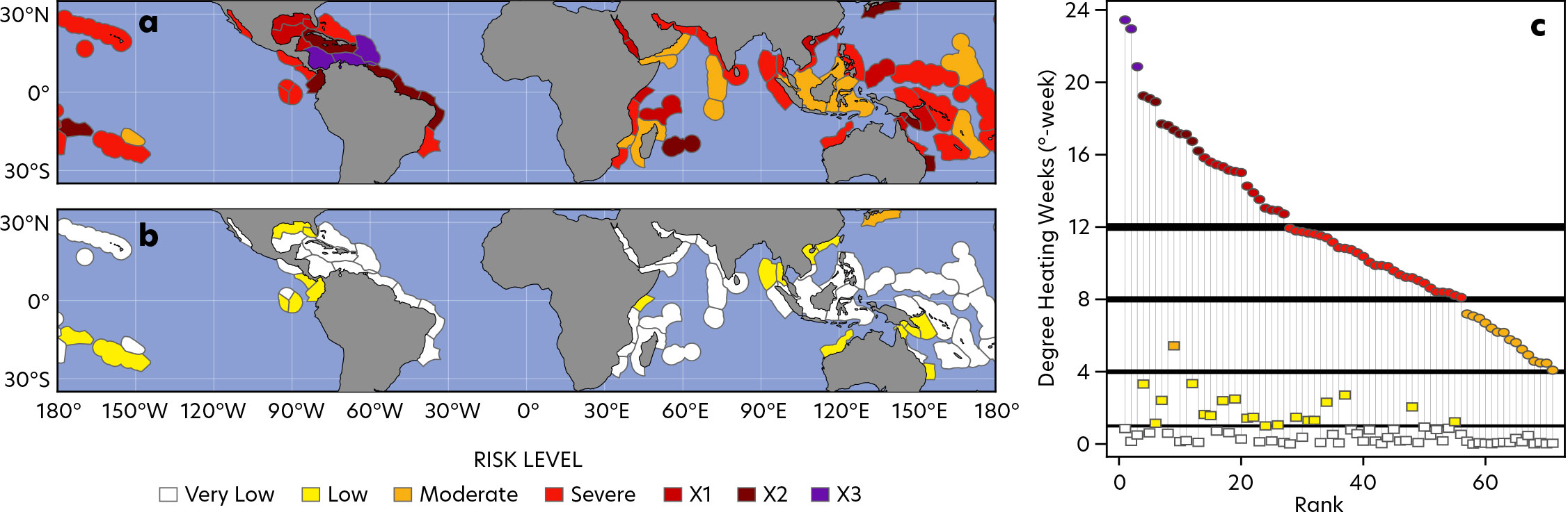
FIGURE 1. Bleaching risk attributable to anthropogenic climate change for the fourth global mass coral bleaching event. (a) Risk levels based on maximum degree heating weeks (DHWmax) for 71 regions where bleaching was reported during 2018–2025 (Spady et al., 2026). The extreme risk level is split into three sublevels to highlight the gradation. (b) Risk levels calculated using counterfactual temperatures. (c) Plot of observed (circles) and counterfactual (squares) DHWmax. The regions are ranked based on the observed values and colored according to risk levels as in panel a. The DHWmax values for each region are in online supplementary Table S1. > High res figure

 

The influence of climate change is also apparent in previous global coral bleaching events. During each of these events, at least 40 regions were at moderate risk (Figure 2). In 1998, only one of these regions had bleaching risk that was not attributable, meaning that the region reached the moderate risk level under the counterfactual conditions (in the absence of global warming). For all other global events, the other regions would not have had this level of risk in the counterfactual climate. The rising trend in the number of regions experiencing each risk level suggests that many regions are now experiencing stressful temperatures multiple times in a decade.

 

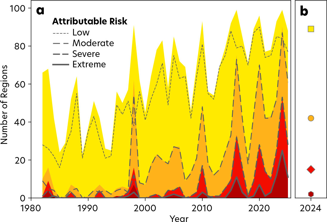
FIGURE 2. Number of coral regions exposed to elevated risk of bleaching. (a) Number of regions reaching a particular bleaching risk level (indicated by colors as in Figure 1a). The dashed lines show the number of regions where the risk is attributable to human-induced warming, meaning that the region’s DHWmax calculated with observed temperatures is above the threshold but the value using the counterfactual temperatures is below the threshold. (b) The number of regions at each risk level in 2024 re-calculated using the 1992–2023 baseline. > High res figure

 

Global Warming vs. El Niño

The attributability of the 1998 event is especially noteworthy given the perceived importance of El Niño in that event (Hoegh-Guldberg, 1999; Bruno et al., 2001). Our approach to calculating the counterfactual temperature is designed to account for natural variability from the El Niño-Southern Oscillation (ENSO) and other sources. It does this by characterizing the distribution of temperatures during a 30-year reference period (in this case, 1991–2020) and then shifting that distribution using the observed trends and climate models (Giguere et al., 2024). This means that the counterfactual temperatures for 1998 or any El Niño year would reflect El Niño conditions in the absence of warming.

To further explore the hypothesis that global warming and not El Niño is the main driver of large-scale bleaching, we use linear regression to fit a statistical model of DHW_max for each region:

DHW_max(year) = a*GMT15(year) + b*ONI(year-L) + c,

where ONI(year) is the monthly Oceanic Niño Index (Glantz and Ramirez, 2020; NOAA, 2025) from the month when the region’s maximum monthly climatological temperature occurs. The parameter L is the lag in months (from 0 to 12) that gives the best fit. We found 23 regions where only the temperature term was significant and 74 out of 100 regions where both the global temperature and ONI effects were significant (Figure S1 in the online supplementary material). For the regions where both factors were significant, we calculated GMT_eqiv = 2*b/a (i.e., the global mean temperature that leads to a change in DHW_max comparable to a strong El Niño; ONI = 2).

According to the statistical modeling, the effect of global temperature became stronger than El Niño in half the regions where both factors are significant when global mean temperature was only 0.5°C above the preindustrial (Figure 3a, blue curve). These conditions occurred in the year 1989. In 1998, during the first global bleaching event, the global mean temperature was 0.72° above preindustrial conditions, and warming was stronger in 61 out of 74 regions. Under current conditions in 2025 (GMT15 = 1.35°), only three regions, Cocos Islands, Northern Galápagos Islands, and Line Islands, have a stronger El Niño effect (Figure 3b). Under current warming rates (SSP3-7.0), warming will outweigh ENSO in all regions where both factors are significant by 2028.

The statistical models also demonstrate that climate change has been the main driver of coral bleaching risk over the last 40 years. By 2000, when GMT15 = 0.77°C, the effect of warming emerged from natural variability in half of the 95 regions with significant GMT15 terms (Figure 3a). In the current climate of 1.35°C, forcing from global temperature exceeds natural variability in 93% of regions (90/97). All regions are expected to exceed their natural variability by 2040 (Figure 3c).

 

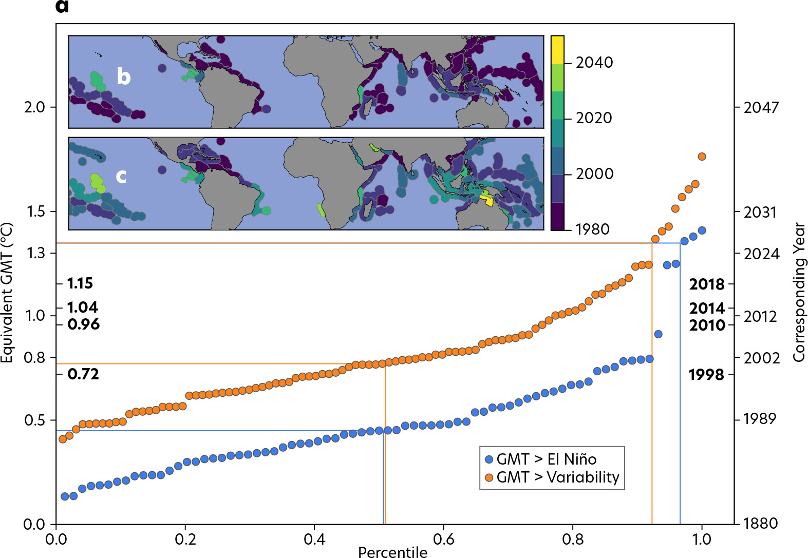
FIGURE 3. Drivers of bleaching risk. (a) The number of regions (expressed as a percentile) for which the influence of global mean temperature (GMT) on DHWmax exceeds that of a strong El Niño (blue dots) or natural variability (orange dots). The year when the equivalent GMT value was or is expected to be reached is indicated on the right. The GMT values for the start of the four global mass bleaching events are indicated in bold. One set of thin lines indicates the equivalent GMT when the GMT effect is stronger in 50% of regions. The other set highlights the proportion of regions where GMT is stronger in 2025 (current climate of 1.35°C). The maps show the decade in which the effect of GMT exceeds that of El Niño (b) or natural variability (c). > High res figure

 

Discussion

Both the attribution analysis and the linear modeling indicate that rising greenhouse gas emissions and the ensuing rise in global temperatures are the main drivers of mass coral bleaching. Without human-induced climate change, reef-wide bleaching would be exceedingly rare, and global bleaching events simply would not occur. According to our analysis, large El Niño events add to the risk from long-term warming, but temperature changes from El Niño would not be strong enough on their own to result in widespread bleaching.

The main advance in our study is the ability to quantify the influence of global warming and to isolate it from natural climate variability, including El Niño events. The multi-method, daily approach developed by Giguere et al. (2024) is currently being used to provide operational assessments of the influence of climate change on sea surface temperatures (see https://csi.climatecentral.org/ocean). This approach provides a convenient pathway for generating time series of counterfactual temperatures that can be used for impact attribution. The main requirement for impact attribution is a model linking sea surface temperature with the process of interest. Marine species distributions (e.g., Morley et al., 2018) and fishery population dynamics (e.g., Pershing et al., 2015) have all been modeled using sea surface temperature and would be particularly suited to attribution studies.

The DHW risk model follows from the understanding that reef-building corals are adapted to the prevailing conditions in their regions. Exposure to stressful temperatures can cause bleaching; however, it can also lead to physiological acclimatization and genetic adaptation, and at the community level, to the loss of the species most sensitive to warming. This may explain why some reefs do not bleach when exposed to conditions that they have previously experienced. For example, in the Chagos Archipelago, high DHW values in 2005 and 2010 were comparable in magnitude to the 1998 event, yet coral cover did not decline and instead increased until 2015 (Sheppard et al., 2017).

Ultimately, a region will only be able to retain a coral reef ecosystem if the rate of adaptation (defined broadly to include processes ranging from acclimatization and genetic changes to species replacement) is faster than the rate of warming (Pershing et al., 2019). Understanding the process of adaptation to rising temperatures is the defining goal of climate change ecology (Witman et al., 2023). The rate of adaptation in coral reef communities should be slow due to the long lifespan and slow growth of most reef-​building corals and will be further exacerbated in isolated reefs where species replacement is slower.

Defining bleaching risk relative to the original baseline period echoes the fixed-baseline definition of marine heatwaves (Hobday et al., 2016). Jacox (2019) argued for defining marine heatwaves after removing the long-term trend. From the perspective of marine ecology, removing the trend assumes that adaptation processes are fast enough to keep pace with the trend. Coral communities lie somewhere between these perspectives. If we shift the baseline period for the DHW calculations from the standard NOAA period (mean year = 1982.3) to the most recent 30 years (mean year = 2008.5), there is a reduction in the number of reefs at each risk level (Figure 2b); however, the number of reefs exposed in each category remains high and is similar to 1998 and 2010. In other words, we would still expect a significant global mass bleaching event.

Our analysis suggests that anthropogenic warming was already driving coral bleaching in the 1990s, the period when the scientific consensus on human-caused climate change was coming into focus. The failure to reduce greenhouse gas emissions after that time led to an additional 0.7° of warming, increasing the exposure of reef ecosystems to dangerously warm temperatures. The International Union for Conservation of Nature (IUCN) has documented that 1,008 species have gone extinct since 1600, most due to human activities (IUCN, 2025). Continued emissions and additional warming raise the potential that human actions may soon eliminate coral reef ecosystems as we know them from the planet.

 

Acknowledgments

This work synthesizes climate models and Earth system observations produced by agencies all over the world, but especially by NOAA in the United States. We are deeply grateful for these valuable contributions to our ability to track changes on the planet. This manuscript and the analysis were improved by helpful suggestions from Erick F. Geiger, Derek Manzello, Blake L. Spady, Alistair Hobday, and two anonymous reviewers. Financial support for this work was provided by the Bezos Earth Fund and the CO2 Foundation (AJP, JG).

Pershing, A.J., J.F. Bruno, J. Giguere, and A. Khrizman. 2026. Quantifying the role of climate change in driving mass coral bleaching. Oceanography 39(2):12–16, https://doi.org/10.5670/oceanog.2026.e210.

• Materials and Methods, Figure S1, and Table S1

1. Bellwood, D.R., T.P. Hughes, C. Folke, and M. Nyström. 2004. Confronting the coral reef crisis. Nature 429(6994):827–833, https://doi.org/10.1038/nature02691.
2. Bruno, J., C. Siddon, J. Witman, P. Colin, and M. Toscano. 2001. El Niño related coral bleaching in Palau, western Caroline Islands. Coral Reefs 20(2):127–136, https://doi.org/​10.1007/s003380100151
3. Fisher, R., R.A. O’Leary, S. Low-Choy, K. Mengersen, N. Knowlton, R.E. Brainard, and M.J. Caley. 2015. Species richness on coral reefs and the pursuit of convergent global estimates. Current Biology 25(4):500–505, https://doi.org/10.1016/​j.cub.2014.12.022.
4. Giguere, J., D.M. Gilford, and A.J. Pershing. 2024. Attributing daily ocean temperatures to anthropogenic climate change. Environmental Research: Climate 3(3):035003, https://doi.org/10.1088/2752-5295/ad4815.
5. Gilford, D.M., A.J. Pershing, B.H. Strauss, K. Haustein, and F.E.L. Otto. 2022. A multi-method framework for global real-time climate attribution. Advances in Statistical Climatology, Meteorology and Oceanography 8:135–154, https://doi.org/10.5194/ascmo-8-135-2022.
6. Gilford, D.M., J. Giguere, and A.J. Pershing. 2024a. Human-caused ocean warming has intensified recent hurricanes. Environmental Research: Climate 3(4):045019, https://doi.org/10.1088/2752-5295/ad8d02.
7. Gilford, D.M., A.J. Pershing, J. Giguere, and F.E.L. Otto. 2024b. Human fingerprints on daily temperatures in 2022. Bulletin of the American Meteorological Society 105(7):E1365–E1370, https://doi.org/10.1175/BAMS-D-23-0264.1.
8. Glantz, M.H., and I.J. Ramirez. 2020. Reviewing the Oceanic Niño Index (ONI) to enhance societal readiness for El Niño’s impacts. International Journal of Disaster Risk Science 11(3):394–403, https://doi.org/10.1007/s13753-020-00275-w.
9. Goreau, T., T. McClanahan, R. Hayes, and A.L. Strong. 2000. Conservation of coral reefs after the 1998 global bleaching event. Conservation Biology 14(1):5–15, https://doi.org/10.1046/j.1523-1739.2000.00011.x.
10. Heron, S.F., L. Johnston, G. Liu, E.F. Geiger, J.A. Maynard, J.L. De La Cour, S. Johnson, R. Okano, D. Benavente, and T.F.R. Burgess. 2016. Validation of reef-scale thermal stress satellite products for coral bleaching monitoring. Remote Sensing 8(1):59, https://doi.org/10.3390/rs8010059.
11. Hobday, A.J., L.V. Alexander, S.E. Perkins, D.A. Smale, S.C. Straub, E.C.J. Oliver, J.A. Benthuysen, M.T. Burrows, M.G. Donat, M. Peng, and others. 2016. A hierarchical approach to defining marine heatwaves. Progress in Oceanography 141:227–238, 10.1016/j.pocean.2015.12.014, https://doi.org/​10.1016/​j.pocean.​2015.12.​014.
12. Hoegh-Guldberg, O. 1999. Climate change, coral bleaching and the future of the world’s coral reefs. Marine and Freshwater Research 50(8):839–866, https://doi.org/​10.1071/MF99078.
13. Hope, P., J. Nahar, G.C. Tolhurst, S.P. Rauniyar, R.C. McKay, L. Zhou, M.R. Grose, B.C. Trewin, D.J. Martin, and S. Grainger. 2024. Lessons learnt from a real-time attribution and contextualisation trial in a national meteorological and hydrological service. Environmental Research: Climate 3(4):045014, https://doi.org/​10.1088/2752-5295/ad7da8.
14. IPCC. 2021. Climate Change 2021: The Physical Science Basis. Contribution of Working Group I to the Sixth Assessment Report of the Intergovernmental Panel on Climate Change. V. Masson-Delmotte, P. Zhai, A. Pirani, S.L. Connors, C. Péan, S. Berger, N. Caud, Y. Chen, L. Goldfarb, M.I. Gomis, and others, eds., Cambridge University Press, Cambridge, United Kingdom and New York, NY, USA, 2,391 pp.,
    https://doi.org/10.1017/9781009157896.
15. IUCN (International Union for Conservation of Nature). 2025. “Summary Statistics.” IUCN Red List of Threatened Species, https://www.iucnredlist.org/resources/summary-statistics#Summary%20Tables.
16. Jacox, M.G. 2019. Marine heatwaves in a changing climate. Nature 571:485–487, https://doi.org/10.1038/d41586-019-02196-1.
17. Lange, S. 2019. Trend-preserving bias adjustment and statistical downscaling with ISIMIP3BASD (v1. 0). Geoscientific Model Development 12(7):3,055–3,070, https://doi.org/10.5194/gmd-12-3055-2019.
18. Laufkötter, C., J. Zscheischler, and T. Frölicher. 202. High-impact marine heatwaves attributable to human-induced global warming. Science 369:1,621–1,625, https://doi.org/​10.1126/science.aba0690.
19. Liu, G., S.F. Heron, C.M. Eakin, F.E. Muller-Karger, M. Vega-Rodriguez, L.S. Guild, J.L. De La Cour, E.F. Geiger, W.J. Skirving, and T.F.R. Burgess. 2014. Reef-scale thermal stress monitoring of coral ecosystems: New 5-km global products from NOAA Coral Reef Watch. Remote Sensing 6(11):11,579–11,606, https://doi.org/​10.3390/rs61111579.
20. Manzello, D.P., R. Cunning, R.F. Karp, A.C. Baker, E. Bartels, R. Bonhag, A. Borreil, A. Bourque, K.T. Brown, and A.W. Bruckner. 2025. Heat-driven functional extinction of Caribbean Acropora corals from Florida’s coral reef. Science 390(6771):361–366, https://doi.org/10.1126/science.adx7825.
21. Morice, C.P., J.J. Kennedy, N.A. Rayner, J.P. Winn, E. Hogan, R.E. Killick, R.J.H. Dunn, T.J. Osborn, P.D. Jones, and I.R. Simpson. 2021. An updated assessment of near-surface temperature change from 1850: The HadCRUT5 data set. Journal of Geophysical Research: Atmospheres 126(3):e2019JD032361, https://doi.org/​10.1029/2019JD032361.
22. Morley, J.W., R.L. Selden, R.J. Latour, T.L. Frolicher, R.J. Seagraves, and M.L. Pinsky. 2018. Projecting shifts in thermal habitat for 686 species on the North American continental shelf. PLoS One 13(5), https://doi.org/10.1371/journal.pone.0196127.
23. NOAA. 2025. ONI_v5. https://www.cpc.ncep.noaa.gov/products/analysis_monitoring/ensostuff/ONI_v5.php.
24. Norström, A.V., M. Nyström, J. Lokrantz, and C. Folke. 2009. Alternative states on coral reefs: Beyond coral-macroalgal phase shifts. Marine Ecology Progress Series 376:295–306, https://doi.org/10.3354/meps07815.
25. Otto, F.E.L. 2017. Attribution of weather and climate events. Annual Review of Environment and Resources 42:627–646, https://doi.org/10.1146/annurev-​environ-​102016-​060847.
26. Pershing, A.J., M.A. Alexander, C.M. Hernandez, L.A. Kerr, A. Le Bris, K.E. Mills, J.A. Nye, N.R. Record, H.A. Scannell, J.D. Scott, and others. 2015. Slow adaptation in the face of rapid warming leads to collapse of the Gulf of Maine cod fishery. Science 350(6262):809–812, https://doi.org/10.1126/science.aac9819.
27. Pershing, A.J., N.R. Record, B.S. Franklin, B.T. Kennedy, L. McClenachan, K.E. Mills, J.D. Scott, A.C. Thomas, and N.H. Wolff. 2019. Challenges to natural and human communities from surprising ocean temperatures. Proceedings of the National Academy of Sciences of the United States of America 116(37):18,378–18,383, https://doi.org/10.1073/pnas.1901084116.
28. Reed, K.A., M.F. Wehner, and C.M. Zarzycki. 2022. Attribution of 2020 hurricane season extreme rainfall to human-induced climate change. Nature Communications 13(1):1905, https://doi.org/10.1038/s41467-022-29379-1.
29. Reynolds, R.W., T.M. Smith, C. Liu, D.B. Chelton, K.S. Casey, and M.G. Schlax. 2007. Daily high-resolution-blended analyses for sea surface temperature. Journal of Climate 20(22):5,473–5,496, https://doi.org/10.1175/2007JCLI1824.1.
30. Sheppard, C., A. Sheppard, A. Mogg, D. Bayley, A.C. Dempsey, R. Roache, J. Turner, and S. Purkis. 2017. Coral bleaching and mortality in the Chagos Archipelago. Atoll Research Bulletin (613):1–26, https://doi.org/10.5479/si.0077-5630.613.
31. Skirving, W.J., S.F. Heron, B.L. Marsh, G. Liu, J.L. De La Cour, E.F. Geiger, and C.M. Eakin. 2019. The relentless march of mass coral bleaching: A global perspective of changing heat stress. Coral Reefs 38(4):547–557, https://doi.org/10.1007/s00338-019-01799-4.
32. Spady, B.L., W.J. Skirving, J.L. De La Cour, E.F. Geiger, G. Liu, O. Hoegh-Guldberg, A. Norrie, S.F. Heron, M.W. Pomeroy, and G. Kolodziej. 2026. The 4th global coral bleaching event: Ushering in an era of near-annual bleaching. Coral Reefs, https://doi.org/10.1007/s00338-025-02810-x.
33. Spalding, M.D., H.E. Fox, G.R. Allen, N. Davidson, Z.A. Ferdaña, M.A.X. Finlayson, B.S. Halpern, M.A. Jorge, A.L. Lombana, and S.A. Lourie. 2007. Marine ecoregions of the world: A bioregionalization of coastal and shelf areas. BioScience 57(7):573–583, https://doi.org/10.1641/B570707.
34. Stott, P.A., D.A. Stone, and M.R. Allen. 2004. Human contribution to the European heatwave of 2003. Nature 432(7017):610–614, https://doi.org/10.1038/nature03089.
35. Strauss, B.H., P.M. Orton, K. Bittermann, M.K. Buchanan, D.M. Gilford, R.E. Kopp, S. Kulp, C. Massey, H. de Moel, and S. Vinogradov. 2021. Economic damages from Hurricane Sandy attributable to sea level rise caused by anthropogenic climate change. Nature Communications 12(1):2720, https://doi.org/10.1038/s41467-021-22838-1.
36. Swain, D.L., D. Singh, D. Touma, and N.S. Diffenbaugh. 2020. Attributing extreme events to climate change: A new frontier in a warming world. One Earth 2(6):522–527, https://doi.org/10.1016/j.oneear.2020.05.011.
37. UNEP WCMC (United Nations Environment Programme World Conservation Monitoring Centre). 2025. Ocean+ Habitats, https://doi.org/10.34892/fpe3-ar97.
38. Van Oldenborgh, G.J., K. van der Wiel, A. Sebastian, R. Singh, J. Arrighi, F. Otto, K. Haustein, S. Li, G. Vecchi, and H. Cullen. 2017. Attribution of extreme rainfall from Hurricane Harvey, August 2017. Environmental Research Letters 12(12):124009, https://doi.org/10.1088/1748-9326/aa9ef2.
39. Witman, J.D., A.J. Pershing, and J.F. Bruno. 2023. Smooth and spiky: The importance of variability in marine climate change ecology. Annual Review of Ecology, Evolution, and Systematics 54:129–149, https://doi.org/10.1146/annurev-ecolsys-022323-082123.

This is an open access article made available under the terms of the Creative Commons Attribution 4.0 International License (https://creativecommons.org/licenses/by/4.0/), which permits use, sharing, adaptation, distribution, and reproduction in any medium or format as long as users cite the materials appropriately, provide a link to the Creative Commons license, and indicate the changes that were made to the original content. Images, animations, videos, or other third-party material used in articles are included in the Creative Commons license unless indicated otherwise in a credit line to the material. If the material is not included in the article’s Creative Commons license, users will need to obtain permission directly from the license holder to reproduce the material.