The tropical Pacific is one of the largest ocean regions on Earth where the trace element iron limits new primary production and therefore the efficiency of carbon export to the deep sea. Although there is a long history of marine biogeochemical research in the tropical Pacific, recent advancements using GEOTRACES key parameters such as iron and nitrate isotopes (nitrate δ¹⁵N and δ¹⁸O) make this a good time to review the current understanding of tropical Pacific nitrate dynamics—how both regional subsurface nitrate characteristics and surface ocean nitrate utilization change with time. While this article provides a comprehensive overview of the biological, chemical, and physical processes shaping equatorial Pacific subsurface-to-surface nutrients, it principally explores the findings from the first nitrate isotope time series in iron-limited high nutrient, low chlorophyll waters. Results indicate that the preferential recycling of bioavailable iron within the euphotic zone is required to explain even the lowest observed nitrate utilization in the eastern equatorial Pacific (EEP). Furthermore, because seasonal-to-interannual nitrate utilization variability in the EEP cannot be driven by changes in iron supply, this work argues that iron recycling (and therefore bioavailable iron) is modulated by upwelling rate changes, creating a predicted and recently observed spectrum of iron limitation in the iron-limited EEP surface waters. In other words, upper ocean physics overwhelmingly dominates seasonal-to-interannual nitrate utilization in the iron-​limited EEP. This new understanding of nitrate utilization in iron-limited waters helps to explain long-term changes in past equatorial Pacific nitrate utilization obtained via sedimentary proxy records and potentially complicates the efficacy of future iron fertilization of the equatorial Pacific.

Global nitrate δ15N data visualization. From Rafter et al. (2019). > High res figure

Introduction

Marine primary production is traditionally separated into “new production” fueled by nitrogen delivered to the euphotic zone and “regenerated production” fueled by ammonium produced after organic matter remineralization (Dugdale and Goering, 1967). The “new” nitrogen could be either dissolved N₂ or nitrate (NO₃^–) that is upwelled to the euphotic zone. The latter is the focus of this article. Distinguishing between new and regenerated production provides a practical method for quantifying net carbon export from the global surface ocean. The simple, yet effective assumption in Eppley and Peterson (1979) is that a mass balance of upper ocean elements requires nitrate-​fueled new production (i.e., “new” nutrient utilization) to be “quantitatively equivalent to the organic matter that can be exported in the euphotic zone without the production system running down.” Consequently, incomplete utilization of nitrate in many parts of the surface ocean can be considered a missed opportunity for phytoplankton to fix inorganic carbon, build biomass, and—via export to the deep sea—sequester carbon (i.e., CO₂) from the atmosphere (e.g., see Ito and Follows, 2005; Hain et al., 2010; Sigman et al., 2010).

At the global scale, nitrate persists in high nutrient, low chlorophyll (HNLC) regions because phytoplankton growth, nitrate utilization, and organic carbon fixation and export are limited by iron (Coale et al., 1996; J.K. Moore et al., 2001; C.M. Moore et al., 2013). Ocean regions with surface ocean nitrate concentrations >1 µmol kg^–1 are colored pink in Figure 1a to illustrate surface waters where iron limitation reduces nitrate utilization and new primary production. Accordingly, relieving the iron limitation of HNLC waters is invoked to explain past changes in the atmospheric concentrations of the greenhouse gas CO₂ and therefore climate (Martin, 1990; Hain et al., 2010; Martinez-Garcia et al., 2014; Sigman and Boyle, 2000). A more complete understanding of marine iron cycling is also critical for a wide range of applications, such as predicting future changes in higher tropic level biomass (Tagliabue et al., 2020) and the deliberate iron fertilization of HNLC regions to enhance marine carbon dioxide removal (NASEM, 2021).

 

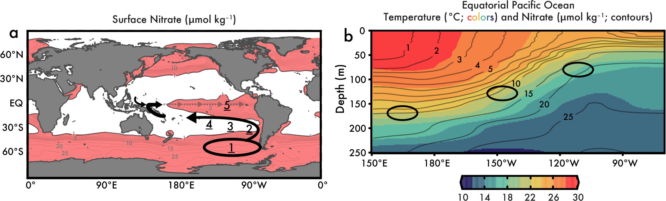
FIGURE 1. While the characteristics of tropical Pacific thermocline nitrate depend on global processes, they also reflect local physics. (a) Global surface nitrate concentrations greater than 1 μmol kg–1 (Garcia et al., 2019) are colored pink to indicate the primary limitation of phytoplankton growth (and nitrate utilization) by iron (see Coale et al., 1996; J.K. Moore and Doney, 2007; C.M. Moore et al., 2013). The arrows in (a) indicate the higher latitude resupply routes of equatorial Pacific nitrate (and other nutrients) as described in the literature (Toggweiler et al., 1991; Palter et al., 2010; Rafter et al., 2012, 2013), with arrow size qualitatively representing the hemispheric contributions to the Equatorial Undercurrent (as estimated by Lehmann et al., 2018). See text for description of processes (steps) indicated by underlined numbers. (b) Equatorial Pacific nitrate concentrations with depth (isolines) closely correspond to temperatures (colors) toward the surface, illustrating the shared influence of upper ocean physics (i.e., Chavez et al., 1999; Rafter and Sigman, 2016). The location of the data in (b) is shown by the dotted line in (a). Ovals in (b) demark some of the calculated depths for waters upwelled to the surface in Rafter and Sigman (2016). > High res figure

 

A particular area of ongoing marine iron cycling research concerns its relationship to nitrate utilization in HNLC waters (Tagliabue et al., 2014, 2016), with some studies complicating the historic understanding that new production (i.e., fueled by nitrate) is based on “new nutrients” upwelled from below (Rafter et al., 2017).

This article provides a thorough assessment of nitrate dynamics in the iron-​limited tropical Pacific, moving from the “upstream” influences on subsurface nutrients to the temporal variability of nitrate utilization and its relationship to iron in EEP surface waters. The tropical Pacific is an excellent natural laboratory for investigating the temporal variability of nitrate and iron utilization (Chavez et al., 1999; Murray et al., 1994; Strutton et al., 2008, 2011) because of its long history of biogeochemical research (e.g., the JGOFS and EB04 cruises; Murray et al., 1997; Nelson and Landry, 2011) and the large, predictable, seasonal-​to-​interannual changes in tropical Pacific upwelling strength and thermocline depth (Wyrtki, 1981; Xie, 1994). Although tropical Pacific biogeochemistry is relatively well studied (Martin et al., 1994; Chai et al., 1996; Coale et al., 1996; Fitzwater et al., 1996; Chavez et al., 1999; Gorgues et al., 2010; Kaupp et al., 2011; Strutton et al., 2011; Saito et al., 2020; Browning et al., 2023), fundamental aspects of nitrate supply and uptake have only recently been addressed. Specifically, the following questions are considered here: (1) What is the biogeochemical history of the nitrate (and other nutrients) that resupply the low latitude Pacific surface waters? (2) How are these waters/​nutrients moved to the equatorial Pacific surface? (3) What is the temporal variability of nitrate utilization in tropical Pacific surface waters? (4) What does the variability of EEP nitrate utilization tell us about iron cycling and the controls of new production in this HNLC? (5) What are the implications of these findings for interpreting past and predicting future changes in iron and nitrate dynamics in HNLC waters?

This review addresses these questions by considering a wide range of research that includes biological, geological, chemical, and physical oceanography in addition to seasonal-to-​interannual climate variability (Xie, 1994; Trenberth et al., 1998; Wang and Fiedler, 2006). In particular, this text places a strong emphasis on the scientific insights gleaned from nitrogen isotopic measurements of both seawater nitrate and marine sediment (e.g., Rafter and Charles, 2012; Rafter and Sigman, 2016). As is the case for the GEOTRACES program, the application of these seawater- and sedimentary-​based measurements aim to inform our understanding of marine biogeochemistry today and in the past (by proxy) (GEOTRACES Planning Group, 2006). While only some of the results described here are products of the GEOTRACES program (e.g., Peters et al., 2017), the insights into EEP nitrate and iron dynamics provide testable predictions for other HNLC waters, which future work can explore, thanks to GEOTRACES.

Note that readers who are not isotope specialists have been carefully considered in this text, so that the insights gleaned from the nitrate isotope measurements about nitrate and iron dynamics in an HNLC region can be more widely understood. For a more advanced treatment of nitrate isotopes, please see the work of Casciotti et al. (2024, in this issue).

 

Nitrate Isotopes: A Unique Geochemical Toolkit

The N and O isotopic compositions of nitrate can, together, provide insight to a variety of processes such as the consumption and production of nitrate (Altabet and François, 1994; Casciotti et al., 2002; Granger et al., 2008). Because of mass-​dependent effects, the lighter isotopes of both N and O (¹⁴N and ¹⁶O, respectively) are utilized by phytoplankton in preference to their heavier isotopes (e.g., ¹⁵N and ¹⁸O). This preferential isotopic utilization increases ¹⁵N/¹⁴N and nitrate ¹⁸O/¹⁶O as nitrate is utilized and as nitrate concentrations decline (to the left of the red circles in Figure 2). The N and O isotopic composition is reported as delta (δ) values via these equations:

δ¹⁵N = [(¹⁵N/¹⁴N_unknown) / (¹⁵N/¹⁴N_standard)] – 1         (1)

(standardized to atmospheric N₂ and multiplied by 1,000 to give units of per mil) and

δ¹⁸O = [(¹⁸O/¹⁶O _unknown) / (¹⁸O/¹⁶O_standard)] – 1         (2)

(standardized to standard mean ocean water [SMOW] and multiplied by 1,000 to give units of per mil).

 

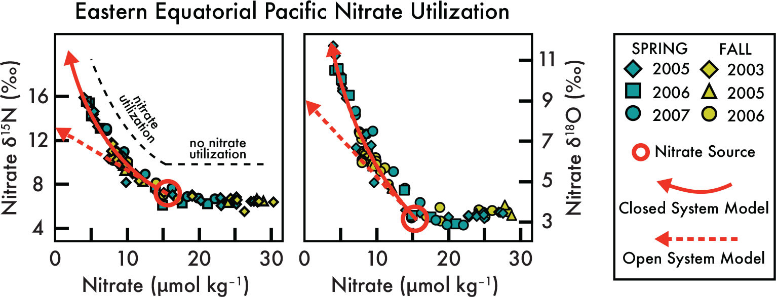
FIGURE 2. Observations of nitrate concentration and nitrate δ15N and δ18O from the eastern equatorial Pacific. These observations (symbols) are from a time series of measurements in the upper 200 m at 0°N, 110°W (first shown in Rafter and Sigman, 2016). Moving from the deepest measurements (on the right; higher nitrate concentration) to the surface (left), there is a reduction in nitrate concentration from ≈30 to 15 µmol kg–1 with negligible changes in nitrate δ15N and δ18O. At approximately 15 µmol kg–1 (circle), nitrate concentrations decline alongside increases in nitrate δ15N and δ18O. The curved red arrows represent a Rayleigh (i.e., a “closed system”) isotopic fractionation alongside nitrate utilization by phytoplankton (for more details, see Mariotti et al., 1981; Sigman and Casciotti, 2001) that is only informed by the nitrate characteristics in the circle ([NO3–] = 15.8 µmol kg–1, nitrate δ15N = 7.1‰, and nitrate δ18O = 3.0‰). The solid red arrows fit the data much better than the “steady state” isotopic fractionation represented by the dashed red arrows (see statistics in Rafter and Sigman 2016), indicating that nitrate—and all equatorial thermocline water—is upwelled to the surface without significant mixing with the subsurface source. In other words, equatorial Pacific nitrate isotopes indicate that upwelling occurs as a parcel of water with limited mixing with the deeper thermocline. > High res figure

 

The curved red line in Figure 2 shows the predicted nitrate concentration and nitrate δ¹⁵N and δ¹⁸O with a “closed system” isotopic fractionation and a fixed isotope effect (as detailed in (Altabet and François, 1994; Sigman and Casciotti, 2001):

δ¹⁵N_reactant or δ¹⁸O_reactant = δ¹⁵N_initial or δ¹⁸O_initial – ε {ln(f)}         (3)

(closed system approximation by Mariotti et al., 1981), where “reactant” is the residual nitrate, “initial” is the subsurface source of nitrate (i.e., before nitrate utilization in the euphotic zone has altered the nitrate characteristics), epsilon (ε) is the isotope effect and “f” is the fraction of nitrate remaining (relative to the initial, subsurface source nitrate concentration). This “Rayleigh” or “closed system” model (Equation 3) assumes no mixing with nitrate outside of this system, such as with the higher nitrate concentrations of the subsurface source. This contrasts with a “steady state” or “open system” model, which allows for mixing between the surface and subsurface alongside nitrate utilization, calculated with the following equation:

δ¹⁵N_reactant or δ¹⁸O_reactant = δ¹⁵N_initial or δ¹⁸O_initial + ε (1–f).         (4)

The straight dashed lines in Figure 2 illustrate the predicted nitrate concentration and nitrate concentrations versus δ¹⁵N and δ¹⁸O for the open system model using the same initial nitrate δ¹⁵N and δ¹⁸O and nitrate concentration as the closed system model (solid, curved lines in Figure 2).

These models for nitrate utilization can be used to estimate the subsurface source water nitrate characteristics and therefore all the initial characteristics of upwelled water before they are altered by primary production—an insight that is only provided by the “nitrate isotope toolkit.” By finding the model parameter values in Equations 3 and 4 that best fit the measured nitrate concentration and isotopes (Rafter and Sigman, 2016), such as with a five-year time series of EEP station occupations in Figure 2, the subsurface source or “initial conditions” of EEP upwelling water are revealed (the red circles in Figure 2). This method assumes that upwelled nitrate concentrations are only lowered by utilization (versus dilution), but this is likely a sound assumption in upwelling regions (e.g., see the discussion of the equatorial Pacific steady state nitrate conservation equation in Rafter and Sigman, 2016). The addition of nitrate via organic matter remineralization/​nitrification (Casciotti and Buchwald, 2012; Granger et al., 2013; Sigman et al., 2005, 2009; Wankel et al., 2007) can also impact this calculation, but the differential isotopic impact from nitrification is not observed in the tropical Pacific euphotic zone (Rafter and Sigman, 2016). See Casciotti et al. (2024, in this issue) for more information, as well as Casciotti et al. (2002) and Granger et al. (2009).

 

High- to Low-Latitude Influences on Tropical Pacific Nutrient Characteristics

Primary production in the surface ocean converts nutrients and carbon to organic matter, much of which sinks out of the surface layer. Therefore, over time, all upper ocean waters require that nutrients be resupplied. At the global scale, upper ocean nutrients are resupplied by organic matter remineralization/​oxidation at depth followed by their physical transport to shallower depths via global ocean overturning (Fripiat et al., 2021). For most of the global ocean, this resupply pathway entails the upwelling of nutrient-rich waters in the Southern Ocean and their equatorward movement in mode and intermediate waters (Sarmiento et al., 2004; Palter et al., 2010; see arrows in Figure 1a). Similarly, Toggweiler et al. (1991) and Toggweiler and Carson (1995) used nutrient concentrations and other geochemical parameters to explore the large-scale relationship between Southern Ocean upwelling and the tropical Pacific, while Tsuchiya (1981) linked tropical Pacific nutrients to advection within the complicated local subsurface zonal jets.

The use of nitrate isotopes provides even more detail on the higher latitude processes determining tropical Pacific nutrient characteristics and therefore the potential drivers of nutrient variability throughout the region (Rafter et al., 2012, 2013). Figure 1a outlines the sequence for resupplying, and therefore influencing, tropical Pacific nutrients (see underlined numbers): (Step 1) Circumpolar Deep Water is delivered along shoaling isopycnals to the Southern Ocean surface (Talley, 2013). Nitrate isotopes clearly show that nutrients in these high nutrient Southern Ocean surface waters are partially consumed by phytoplankton, which lowers nitrate concentration, and discrimination of the lighter N isotope increases nitrate δ¹⁵N by about 1 per mil (1‰). (The deep-sea weighted-average nitrate δ¹⁵N is estimated at 5.0 ± 0.3‰ [Rafter et al., 2019] and increases to ≈6‰ in subantarctic surface waters [Sigman et al., 1999; DiFiore et al., 2006; Rafter et al., 2013].) Ekman transport moves these waters equatorward, where seasonal mixing/stratification leads to the formation of Subantarctic Mode Water (SAMW) >500 m below the surface (e.g., see Figure 1 in Rafter et al., 2013).

As SAMW moves equatorward and then westward at depth (>500 m) within the South Pacific gyre circulation (Step 2 in Figure 1a), lowering of oxygen and increasing nitrate and phosphate concentrations indicate organic matter remineralization along the way. However, one key piece of information only provided by the nitrate isotopes is that the organic matter remineralized at depth must have relatively elevated δ¹⁵N values (Rafter et al., 2013). Peters et al. (2017) later clarified that this organic matter must be produced within the eastern tropical South Pacific, where extreme nitrate isotope fractionation occurs as marine microbes “breathe” using nitrate during denitrification. Similarly, the very high δ¹⁵N produced in the oxygen-deficient waters of the eastern tropical South Pacific can influence the high- to low-latitude moving nitrate via (Step 3) eddy-diffusive mixing (Johnson and McTaggart, 2010; see Figure 6 in Rafter et al., 2012, for more details). Altogether, the processes occurring between the Southern Ocean and the tropical Pacific further increase SAMW nitrate δ¹⁵N another 1‰ (a 2‰ increase from the deep sea; Sigman et al., 2000; Rafter et al., 2019).

Resupplying the Equatorial Pacific Thermocline

The density surface of SAMW moves from breaching the surface in the subantarctic Southern Ocean to >500 m in the equatorial Pacific—depths where these nutrients can only resupply the local thermocline (see Figure 3 in Rafter et al., 2012) through diapycnal mixing (Toggweiler et al., 1991; Step 4 in Figure 1a). In fact, Rafter et al. (2013) argue that subtropical-​to-tropical changes in SAMW-depth nitrate concentrations, nitrate δ¹⁵N and δ¹⁸O, and salinity can be explained by diapycnal mixing between the deeper SAMW-derived waters and the shallower nitrate-deplete South Pacific gyre waters (Step 4). This diapycnal mixing is consistent with the “single process of thermocline ventilation” (Toggweiler et al., 1991) and is similar to diapcynal mixing of nutrients in the North Atlantic (Jenkins and Doney, 2003). Although speculative, the South Pacific gyre diapycnal mixing may occur as these gyre waters move through the many Polynesian islands (similar to island-induced mixing in the North Pacific; Nishioka et al., 2013). After these formerly SAMW-based nutrients are mixed to shallow density surfaces, the proto-equatorial Pacific thermocline waters follow a well-​established pathway (Step 5) through the western tropical Pacific, contributing 70% or more of the equatorial Pacific thermocline water, with the residual coming from North Pacific Intermediate Waters (Lehmann et al., 2018).

 

Nitrate Isotopes Answer the Question: What is the Source of Equatorial Pacific Upwelling?

There are a variety of complications when estimating the subsurface source of upwelled waters, but nitrate isotopes provide a solid, theory-based approach. The equatorial Pacific is particularly difficult in this respect because the trade winds force both the thermocline and the nitracline to shoal toward the east (Figure 1b). Note that both equatorial Pacific nitrate concentrations (contours) and temperatures (colors) are effectively parallel with depth, illustrating that the same air-sea dynamics drive both subsurface temperatures and nutrient concentrations (Figure 1b).

As discussed above, the equations for nitrate isotope fractionation during utilization (Equations 3 and 4) can be rearranged to solve for the initial nitrate concentrations through an iterative process—​solving for multiple unknowns to find the best fit to the observations. Applying the nitrate isotope approach along the equatorial Pacific (ovals in Figure 1b) shows that the subsurface source of western equatorial Pacific (WEP) surface waters is deeper and has slightly lower nitrate concentrations than the east. However, all equatorial Pacific subsurface source waters have essentially the same nitrate δ¹⁵N (with an average of 7.1 ± 0.2‰) and nitrate δ¹⁸O (with an average of 3.0 ± 0.3‰) (Rafter and Sigman, 2016). We can explain this discrepancy as follows. First, the spatial consistency of subsurface source water nitrate δ¹⁵N and nitrate δ¹⁸O speaks to the lasting impact of diapycnal mixing in the South Pacific outlined in Step 4 of Figure 1a and the section above on Resupplying the equatorial Pacific thermocline. Second, the spatial consistency of subsurface nitrate δ¹⁵N and nitrate δ¹⁸O speaks to minimal impact from nitrification—the microbially mediated two-step oxidation of organic matter to nitrate—which has a predictable, differential impact on these isotopes (Sigman et al., 2009). This negligible impact from nitrification underneath the >10,000 km of relatively productive equatorial Pacific surface waters might be surprising, but the subsurface source waters are also clearly related to the very quick (>50 cm s^–1) eastward, thermocline-bound jet known as the Equatorial Undercurrent (EUC; Johnson et al., 2001). Thus, the fact that there is effectively no change in equatorial Pacific subsurface source water nitrate δ¹⁵N and δ¹⁸O is probably best explained by the rapidity with which the waters are transported across the basin. Finally, Rafter and Sigman (2016) lay out additional lines of evidence supporting the EUC as the subsurface source (assumed as far back as Wyrtki, 1981) and that, via upwelling, these subsurface waters are the dominant source of equatorial Pacific surface waters.

Dissolved and particulate iron are also advected within EUC waters to the eastern equatorial Pacific, possibly picked up as EUC source waters brush past Papua New Guinea (Gordon et al., 1997). The variability of dissolved iron concentrations in western and central equatorial Pacific EUC waters is explored in Rafter et al. (2017), but dissolved iron is expected to be uniformly low in the EEP because of a productivity-scavenging feedback. For example, if dissolved iron were high in the EUC, it would be expected to drive increased nitrate utilization, new primary production, and sinking organic matter in the western and central equatorial Pacific—the subsequent increase in sinking organic matter would then scavenge or strip out the residual dissolved iron (Gorgues et al., 2005; Kaupp et al., 2011). Thus, even though there are various influences on nitrate (and presumably phosphate), the productivity-scavenging feedback argues for consistently low dissolved iron as the EUC subsurface source waters approach the eastern equatorial Pacific.

 

Quantifying Equatorial Pacific Nitrate Utilization

The capability to estimate subsurface source water nitrate (and other) characteristics plus the physics of the equatorial Pacific upwelling (see discussion beginning on page 25 in Rafter and Sigman, 2016) permits quantification of nitrate utilization at all equatorial Pacific sites with a simple vertical profile of nitrate isotopes. Accordingly, Rafter and Sigman (2016) utilized samples acquired alongside the biannual NOAA Tropical-Ocean-Atmosphere program (small symbols in Figure 3a) to quantify the spatial and temporal variability of equatorial Pacific subsurface source waters and surface nitrate utilization. This sampling allowed for multiple occupations of the same stations from the western to the eastern tropical Pacific. An example of a repeated station occupation is shown in Figure 2 for 0°N, 110°W. Here, the nitrate characteristics of water upwelled from the estimated subsurface source (red circle)—​and across several seasons—closely follow the model for nitrate uptake in a closed system (curved red arrow). This closed system model contrasts with the steady state model for nitrate isotopic fractionation (red, dashed arrows in Figure 2), which is a model that allows for mixing with the subsurface source. In fact, the nitrate characteristics of upwelling equatorial Pacific waters best fit the closed system model at nearly all of the 35 stations measured over five years and across the basin (see Table 1 in Rafter and Sigman, 2016).

 

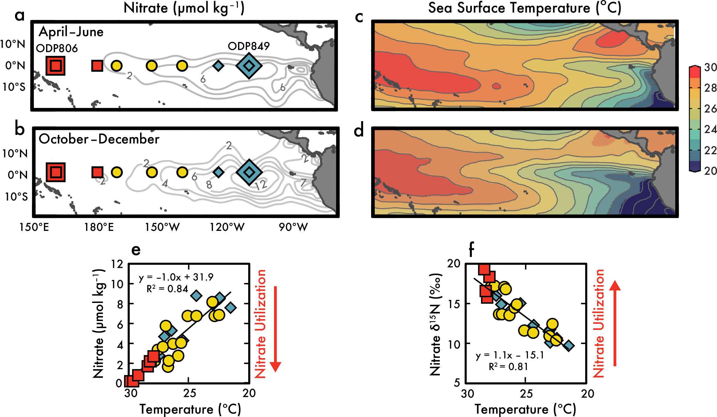
FIGURE 3. The seasonal variability of equatorial Pacific surface nitrate from 2003 to 2008 shown here is not caused by changes in the subsurface source, but rather by changes in nitrate utilization. Seasonal surface nitrate concentrations are highest (contours in a and b) and sea surface temperatures (SST) are lowest (c and d) in the eastern equatorial Pacific during boreal fall, which is also the annual peak period in wind-induced equatorial upwelling (Xie, 1994). Smaller symbols in (a) and (b) represent the locations of nitrate isotope measurements from 2003 to 2008 (Rafter et al., 2012; Rafter and Sigman, 2016), and larger symbols represent the sites of 1-million-year-long sedimentary δ15N records (square: Ocean Drilling Program [ODP] Site 806; diamond: ODP Site 849; Rafter and Charles, 2012). (e) This graph displays a direct comparison of surface mixed layer nitrate concentrations and temperatures from the sites in (a) and (b), indicating a strong, linear correlation with warmer western SST associated with lower surface nitrate concentrations—a correlation that provides no insight to the causation. However, (f) shows that this lowering of nitrate concentrations with warmer SST coincides with another strongly correlated, linear increase in nitrate δ15N, which is diagnostic of increased nitrate utilization alongside the same upper ocean physics that drive changes in equatorial Pacific SST. > High res figure

 

The close fit of the nitrate concentration and isotope measurements to the closed system model in Figure 2 provides several important observations for equatorial Pacific marine biogeochemistry. First, it reveals that upwelled waters undergo minimal mixing as they rise to the surface. Far from an arbitrary observation, the way that equatorial Pacific waters upwell is important because ocean general circulation models and other models typically employ equatorial Pacific upwelling that assumes an open system/continuous supply to the surface (e.g., Chai et al., 1996). Second, it indicates that as waters upwell to the equatorial Pacific surface from their subsurface source in the EUC, phytoplankton utilization drives essentially all changes in nitrate characteristics (Rafter and Sigman, 2016).

Given these discussions of equatorial upwelling and nitrate characteristics, equatorial Pacific nitrate utilization by phytoplankton can be simply calculated by taking the difference between the subsurface source nitrate concentration and the surface mixed layer nitrate. Lateral input to equatorial surface water will be negligible because the physics of Ekman divergence—the poleward movement of upwelled waters once they’ve reached the equatorial surface—limits the lateral input of water along the equator. This is because equatorial upwelling is roughly balanced by divergence at the surface, mostly in the meridional direction (Johnson et al., 2001), and despite strong zonal flows, the average meridional surface water flow causes an upwelled water mass to move from the equator to 1° latitude within a few weeks (Rafter and Sigman, 2016). In other words, even though the zonal gradient in tropical Pacific surface nitrate appears consistent with westward advection of surface waters by the easterly trade winds (Figure 1a), Ekman upwelling and surface divergence make purely zonal surface water advection along the equator physically impossible (see further discussion in Rafter and Sigman, 2016).

Equatorial Pacific Surface Nitrate Utilization and Links to Air-Sea Dynamics

Chavez et al. (1999) elegantly show the interface between equatorial Pacific chemistry and interannual global climate variability, where lowering/​depletion of surface nutrient concentrations in the EEP occurred alongside the warmer sea surface temperature (SST) El Niño phase of the El Niño-Southern Oscillation (ENSO). However, measurements of nitrate concentration changes are not diagnostic of what is driving these changes; they cannot tell us if the lower surface nitrate concentrations during El Niño events were caused by changes in subsurface source water nutrients and/or changes in nitrate utilization. Seasonal changes in equatorial Pacific upwelling offer a similar view to ENSO variability, where the springtime weakening of cross-equatorial trade winds (Xie, 1994) also weakens upwelling and coincides with lower EEP surface nitrate concentrations and warmer SSTs (analogous to an El Niño state) (Figure 3a–d). (In fact, seasonal variance of EEP SST is significantly larger than ENSO-induced variance, as shown in Wang and Fiedler, 2006; see also Figure 1 in Rafter and Sigman, 2016, for updated calculations.) The warm SST and low nitrate concentration relationship observed by Chavez et al. (1999) for El Niño events is also evident for seasonal variability in the Rafter and Sigman (2016) dataset (Figure 3e), showing a linear relationship between all equatorial Pacific mixed layer nitrate and temperature across the basin.

One of the advantages of using nitrate isotopes is that they trace the biogeochemical history of nitrate—and Figure 3f shows that equatorial Pacific surface mixed layer nitrate δ¹⁵N also increases linearly with SST. Because equatorial Pacific nitrate isotopes are diagnostic of nitrate utilization (see text above), the relationship between SST and nitrate isotopes in Figure 3f suggests the upper ocean physics determining equatorial Pacific SST gradient is also influencing nitrate utilization, where warmer SSTs coincide with increased nitrate utilization. This relationship between upper equatorial Pacific physics and nitrate utilization is also apparent in seasonal scale repeat measurements from the EEP (see colors in Figure 2; see Table 1 in Rafter and Sigman, 2016). There is clearly higher nitrate δ¹⁵N and δ¹⁸O, lower nitrate concentrations, and warmer SST during the weaker springtime upwelling season (Figures 2 and 3f)—results that indicate increased nitrate utilization rather than a lower concentration source of nitrate to surface waters.

 

Preferential Cycling of Iron Necessary for Observed Nitrate Utilization in EEP

Considering that iron availability limits nitrate utilization across the tropical Pacific (Martin et al., 1994; Coale et al., 1996; Fitzwater et al., 1996), the relationship between upper equatorial Pacific physics and nitrate utilization (Figures 2 and 3f) was perplexing—the standard way of thinking about nutrient limitation in these iron-limited waters predicts that an increase in nitrate utilization must be accompanied by a change in the iron supply. However, the variability of iron within the EUC is small, and a productivity feedback “upstream”—where enhanced productivity/particle flux would remove iron via scavenging—makes it unlikely to transmit higher source water iron composition to the EEP (Gorgues et al., 2010; Kaupp et al., 2011; also see discussion in Rafter et al., 2017). Observations of EUC iron variability are rare (Slemons et al., 2010; Michael et al., 2021), but low iron concentration variability is expected, given its short residence time (Black et al., 2020; Hawco et al., 2022). Accordingly, seasonal variability in source water iron concentrations is unlikely to explain the observed pattern in equatorial Pacific nitrate utilization. Considering non-marine iron sources, lithogenic (dust-borne) iron supply to the tropical Pacific is already relatively low (Mahowald et al., 2005; Kaupp et al., 2011). Increased winds and therefore lithogenic iron supply during boreal fall would predict increased nitrate utilization when SSTs are generally colder, which is the opposite of what is observed (Figures 2 and 3). Similarly, although lithogenic iron supply can be much larger (arrow sizes in Figure 4 relate to the fluxes), barring inordinate changes in lithogenic iron solubility (i.e., >10 times higher than observed; see Figure 2 in Rafter et al., 2017), changes in lithogenic iron supply (curved dashed arrows in Figure 4) cannot explain the changes in nitrate utilization (see calculations in Rafter et al., 2017). Finally, relatively recent sedimentary archives that are consistent with modern lithogenic Fe flux also suggest minimal dust variability over the past several thousand years (calculated in Rafter et al., 2017, from Winckler et al., 2008).

 

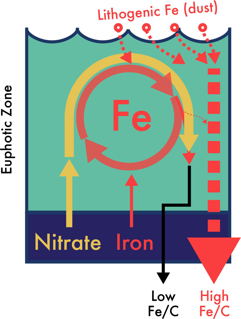
FIGURE 4. Schematic of nitrate and iron flux, utilization, and export in upper equatorial Pacific waters. As detailed in Rafter et al. (2017), the observed nitrate utilization in the iron-limited equatorial Pacific surface waters cannot be explained by the upwelling (solid arrow) or lithogenic/dust-borne (dashed arrows) deliveries of iron. Instead, EEP nitrate utilization must be explained by a differential cycling of iron relative to nitrogen (the circular red arrows), where iron is preferentially cycled/retained and further utilized in the upper equatorial Pacific waters. This model predicts low Fe/C in organic matter sinking out of the euphotic zone (black arrow) and a small loss of iron via scavenging by lithogenic material (very small dashed arrow leaving circular arrows). However, disentangling sinking biogenic Fe/C from the total sinking Fe/C is complicated by the considerably larger flux of high Fe/C lithogenic Fe (dashed arrows). > High res figure

 

Without changes in the external supply of iron, changes in the internal supply of iron via the preferential remineralization of bioavailable iron are needed to explain both the magnitude and the seasonal variability of EEP nitrate utilization (Rafter et al., 2017; Figure 4). A simple accounting of iron supply to the EEP and the nitrate isotope-enabled estimates of nitrate utilization allow us to examine the fundamental relationship between nitrate uptake in iron-limited HNLC waters. For the EEP, Rafter et al. (2017) found that—regardless of physiological requirements—at least an order of magnitude more iron was necessary to explain even the smallest amount of nitrate utilization. By itself, the idea of iron recycling in the upper ocean is not new and has been suggested to support regenerated primary production (i.e., not fueled by nitrate) in the central equatorial Pacific (Hutchins et al., 1993), subantarctic waters (Boyd et al., 2005; Strzepek et al., 2005), and indeed throughout the Southern Ocean (Sieber et al., 2021). Iron recycling was also suggested to extend the lifespan of diatom blooms (Bowie et al., 2001). However, the Rafter et al. (2017) work using the nitrate isotope geochemical toolkit connects the preferential cycling and retention of iron in the upper ocean and nitrate utilization. Considering that nitrate utilization was described by early marine biogeochemists as the key metric for new production and carbon export from the upper ocean (Dugdale and Goering, 1967; Eppley and Peterson, 1979), this link with the preferential cycling of iron complicates the previously assumed segregation between new and regenerated nutrient utilization.

While the exact mechanisms of this preferential iron cycling are still being understood (Barbeau et al., 1996; Boyd et al., 2015, 2017; Bundy et al., 2024; Pham et al., 2022), there are clear signs that HNLC microbial communities work to retain iron in the system. For example, iron-stressed ecosystems can lower their Fe requirements (see Wiseman, 2023, and Wiseman et al., 2023, and references therein). Additionally, retention of much-needed iron may occur by siderophore production (Boiteau et al., 2016; Bundy et al., 2018; Manck et al., 2022), grazing, and viral lysates (Poorvin et al., 2004; Sato et al., 2007). Preferential cycling of iron may help diagnose the shortcomings of biogeochemical models and may be a critical component (along with microbial/​phytoplankton community changes) in predicting changes in primary production throughout the tropical and subtropical Pacific (Browning et al., 2023).

Modulation of Iron Cycling by Upwelling Variability and Future Tests

Explaining the strong relationship between surface nitrate utilization and seasonal upwelling (Figures 2 and 3) in iron-​limited EEP waters requires a physico-​biogeochemical driver linking increased nitrate utilization/iron recycling with reduced upwelling during boreal spring. Model results in Rafter et al. (2017) suggest a link between upwelling and nitrate utilization in iron-​limited equatorial Pacific waters is possible if the residence time in the euphotic zone helps determine the extent of iron recycling (i.e., the number of times iron cycles through the EEP biota; see circle with arrows in Figure 4). Figure 5 provides a schematic of this physico-​biogeochemical relationship, which assumes no change in the phytoplankton community characteristics or the depth of the euphotic zone. In this representation, weaker upwelling (Figure 5a) allows more time for the microbial/​phytoplankton community to recycle iron, thus retaining more of the externally supplied iron and utilizing more nitrate. This required iron recycling likely continues once the equatorial waters reach the surface and are advected poleward, but our ability to quantify nitrate utilization off-equator is degraded when we cannot, with certainty, identify the initial nitrate concentrations.

 

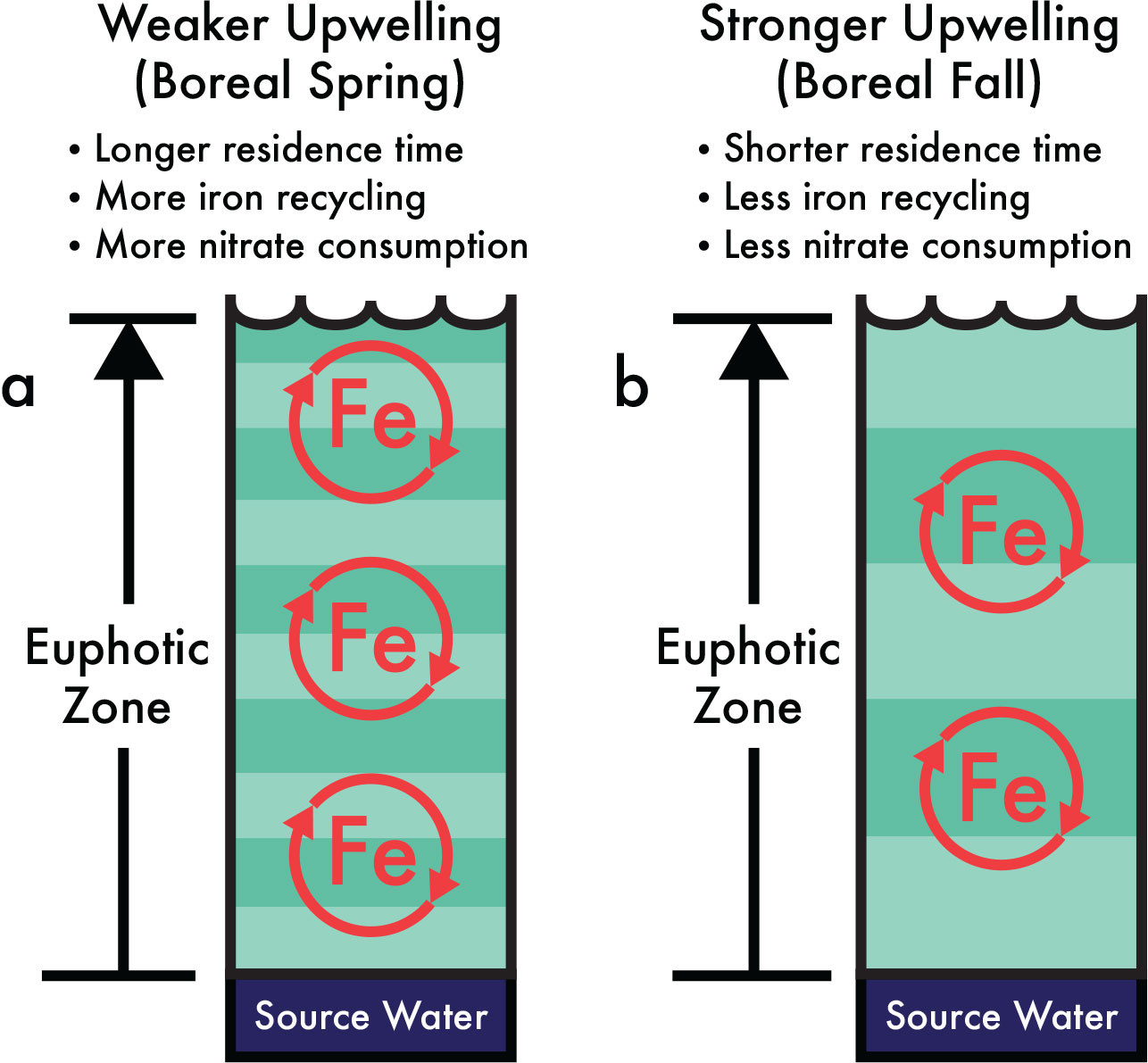
FIGURE 5. Increased nitrate utilization in the iron-limited eastern equatorial Pacific waters can be linked to weaker upwelling if longer residence times allow for more iron recycling. In this conceptual model, the easterly trade winds drive changes in the residence time of equatorial waters as they upwell through a euphotic zone (shown here with a fixed depth). (a) Reduced upwelling/increased residence time of upwelled waters during boreal spring allows for increased iron recycling (illustrated by color banding). (b) Enhanced upwelling/ reduced residence time of upwelled waters during boreal fall do not allow for as much iron recycling. This proposed relationship between upper ocean physics and marine biogeochemistry helps to explain both the observed seasonality of surface nitrate utilization in the iron-limited eastern equatorial Pacific (from nitrate δ15N and δ18O; see Figures 2 and 3) as well as the relationship between long-term changes in seasonal heating and 1-million-​year records of sediment δ15N (see Figure 6). > High res figure

 

The model for iron and nitrogen cycling in iron-limited EEP waters shown in Figure 4 and the physico-​biogeochemical link between iron availability and upwelling illustrated in Figure 5 make several testable predictions. First, the preferential cycling of iron relative to major nutrients like carbon and nitrogen predicts a large deficit in organic matter Fe/C and Fe/N, with exported biogenic material having much lower Fe/C and Fe/N than the living euphotic zone biomass (see bottom of Figure 4). Although living euphotic zone algal Fe/C can be reasonably constrained (e.g., Twining et al., 2011), the biogenic Fe flux out of the euphotic zone will be small compared to the much higher lithogenic Fe flux—the latter can be as much as 97% of the total Fe flux (see the much larger, dashed red arrow in Figure 4; see also Frew et al., 2006; Lamborg et al., 2008; Ohnemus et al., 2019; Tagliabue et al., 2019). Further complications in estimating sinking biogenic Fe fluxes include the recycling and subsequent scavenging of sinking biogenic Fe, producing a relatively large “authigenic” particulate Fe phase in subsurface waters (Tagliabue et al., 2019). Perhaps the details of these processes can be disentangled with future work and constraints on iron isotope fractionation factors (Fitzsimmons and Conway, 2023; König and Tagliabue, 2023).

A second testable prediction of preferential Fe cycling involves its relationship with upwelling. The physico-​biogeochemical relationship in Figure 5 implies that iron limitation is not a binary condition of iron-limited systems but would be more correctly described as an iron limitation spectrum. In this case, the more times that one iron atom is recycled, the more likely some bioavailable iron will be lost, furthering the system along the iron limitation spectrum. Qualitative support for this iron limitation spectrum is shown by ship- and satellite-​based observations that highlight iron-​limited stress increases alongside the predicted increase in iron recycling throughout the tropical and subtropical Pacific (Browning et al., 2023).

Finally, it is likely that preferential iron cycling is a necessary part of marine biogeochemistry in all HNLC regions, although likely modified by local ecology. One testable prediction for the global distribution of preferential iron cycling in iron-limited waters is that the extent of iron recycling necessary to meet the community needs should be less in more iron-rich regions, such as the HNLC waters of the subarctic Atlantic.

 

Analogs of Equatorial Pacific Iron Fertilization

Although the dust-borne iron flux to the tropical Pacific is relatively small, during the last ice age the flux of iron-rich dust to the region was more than double (Winckler et al., 2008) and probably more soluble (Shoenfelt et al., 2017, 2018). The last ice age (and earlier glacial periods) can therefore serve as natural analogs for the purposeful iron fertilization of iron-​limited waters to accelerate the biological carbon pump and lower atmospheric CO₂ (NASEM, 2021). However, there is strong evidence that the naturally elevated iron flux to equatorial Pacific surface waters during the last ice age (and earlier) did not strengthen nitrate utilization, new production, or the efficiency of carbon export to the deep sea (Costa et al., 2016; Winckler et al., 2016). Instead, despite a doubling of iron-rich dust flux during the Last Glacial Maximum, these paleoceanographic studies tell us that the utilization of nitrate and the strength of the biological carbon pump were relatively weak—as is observed today (Murray et al., 1994).

More supporting evidence comes from a study that specifically addresses nitrate utilization in the EEP by using measurements of sediment δ¹⁵N from the western equatorial Pacific (large red square in Figure 3a) and the eastern equatorial Pacific (large blue diamond in Figure 3a) (Rafter and Charles, 2012). In this study, EEP nitrate utilization is reconstructed by taking the difference between western and eastern sediment δ¹⁵N measurements (Δδ¹⁵N; see red line in Figure 6), which constrains and removes changes in the equatorial Pacific subsurface source nitrate δ¹⁵N to provide a 1-million-year record of EEP nitrate utilization. In contrast to expectations for iron fertilization of the EEP by iron-rich glacial dust (at 100,000-year timescales; bottom of Figure 6), EEP nitrate utilization over the past 1 million years is dominated by 19,000–23,000-year cycles. These results, plus independent studies of equatorial Pacific primary production/nitrate utilization (Costa et al., 2016; Winckler et al., 2016), indicate a limited impact on EEP nitrate utilization from dust. Why these analogs for deliberate iron fertilization do not indicate increased nitrate utilization or productivity is unknown, but this perhaps suggests a threshold for iron fertilization that is above glacial increases in iron supply but below the deliberate iron addition experiments (Martin et al., 1994; Coale et al., 1996; Fitzwater et al., 1996). Regardless, these analogs suggest a potentially more complicated role for future iron fertilization in the region.

 

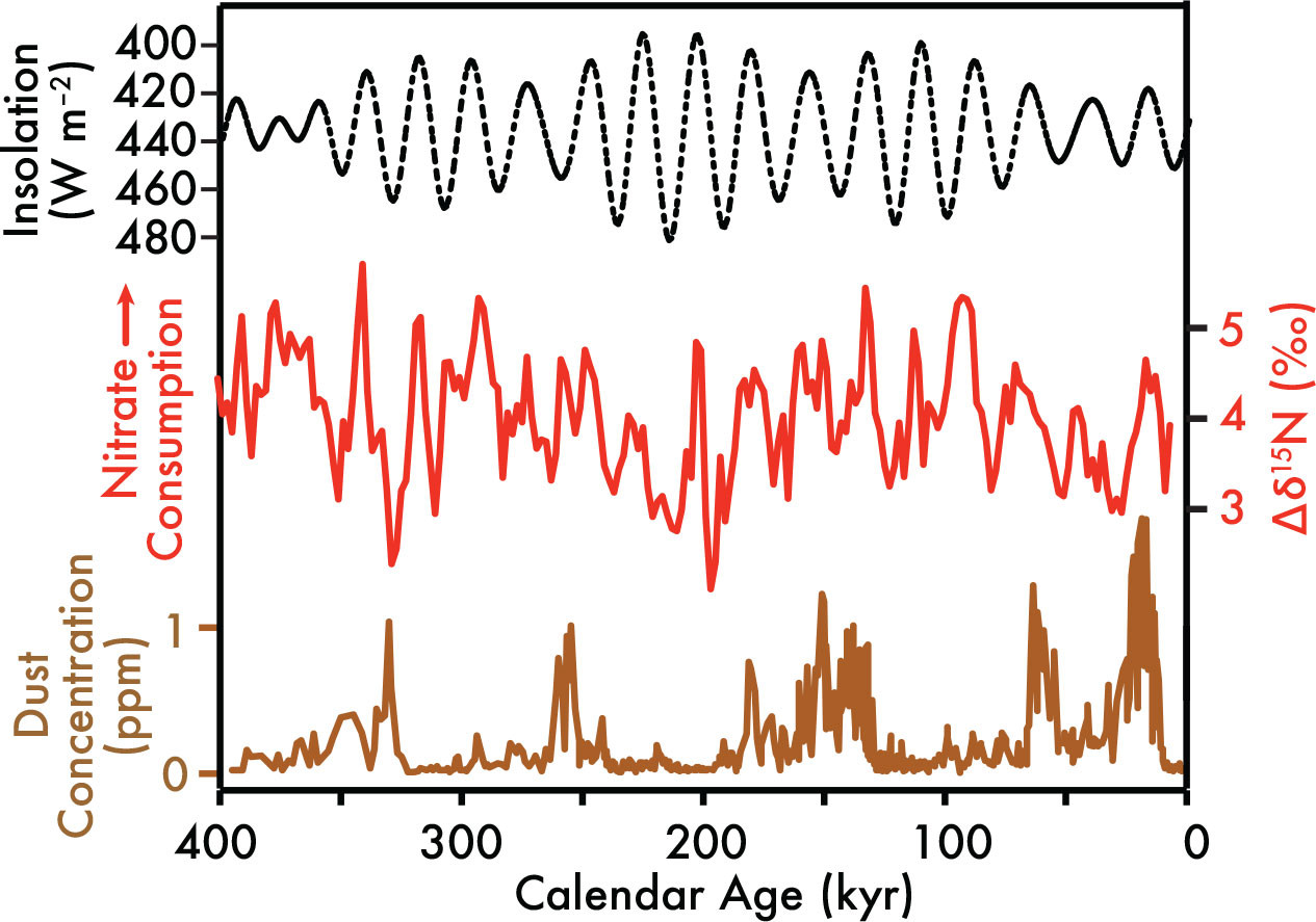
FIGURE 6. Orbital variability induces predictable changes in equatorial Pacific seasonal heating and upwelling that can help explain long-term (19,000 to 23,000 years) variability in eastern equatorial Pacific nitrate utilization. Changes in Earth’s orbit have minimal impacts on annual insolation in the tropics but can adjust the time of year when insolation is greatest (Laskar et al., 2004; note y-axis is flipped). The dashed line (top) shows changes in insolation at the equator during boreal fall, which is a time period suspected to influence millennial and longer-term changes in equatorial Pacific seasonality (Clement et al., 1999). The red line (middle) is the difference between western and eastern equatorial Pacific sediment δ15N (sites are shown in Figure 3a), which records changes in EEP nitrate utilization (Rafter and Charles, 2012). The bottom line is the dust record from the Antarctic icecore, showing the strong 100,000-year periodicity of iron-rich dust in the atmosphere (Petit et al., 1990). > High res figure

 

Do Changes in Seasonality Affect EEP Iron Recycling?

Instead of dust-born iron fertilization, variability in iron recycling may drive both seasonal nitrate utilization (Rafter et al., 2017; Figure 5) and the longer-​term changes in EEP nitrate utilization recorded in sediments (Figure 6). Rafter and Charles (2012) specifically argue that orbitally induced changes in seasonal heating and upwelling on 19,000–23,000-year timescales can drive long-​term changes in EEP upwelling rates, as predicted in Clement et al. (1999). In this model, when seasonal heating is weak during boreal fall, the equatorial Pacific’s “ocean dynamical thermostat” (Clement et al., 1996) works to amplify the already dominant boreal fall upwelling in the EEP (Xie, 1994) on 19,000–23,000-year time­scales (Clement et al., 1999). Strikingly, these orbitally induced changes in seasonal heating/EEP upwelling are coherent and in phase with the EEP nitrate utilization record in Figure 6 (see statistics in Rafter and Charles, 2012). Our developing understanding of iron recycling in HNLC waters leads to the proposition that orbitally induced changes in EEP upwelling also determine nitrate utilization via changes in the degree of iron recycling. These findings about past nitrate utilization in HNLC waters may also be important for considering future changes in marine biogeochemistry resulting from global warming (Richon and Tagliabue, 2021).

 

Concluding Thoughts

The GEOTRACES logo reveals to us that there is more to this program than high-quality measurements of marine trace elements and isotopes. The logo shows an arrow moving to the left, but the arrow “wiggles” over planet Earth—​symbolism that surely reflects the program’s core interest in understanding how Earth systems “change” (the wiggles) with time (the arrow). In fact, the GEOTRACES planning document is full of change, with “climate change,” “past changes,” “future change,” and more appear 146 times (GEOTRACES Planning Group, 2006). Keeping with this aesthetic, the text above could be summarized by the following questions: How did the N and Fe relationship in the tropical Pacific change in the past? What do these past changes tell us about N and Fe cycling today? And, what can we learn from the past and the present to inform the future of N and Fe cycling in iron-limited waters? Far from being the final discussion on this matter, I hope my examination above will be challenged and, if wrong, that these findings will also change.

In my final note, I want to say that I was able to begin answering these questions by using time-series measurements from repeat hydrographic station occupations and sediment cores. Looking ahead, I hope that other researchers will identify the utility and the positive feedback that can occur when bringing together seawater measurements, sediment proxy records, and more. For example, in contrast to the flow of the text above, it was the paleoceanographic records developed in Rafter and Charles (2012) that instigated the subsequent series of primarily seawater-based measurements.

I want to thank the GEOTRACES organizers and the National Science Foundation for their support as well as the editors of this volume for the invitation to provide this perspective.

 

Acknowledgments

The author wants to first thank Christopher D. Charles, Lihini Aluwihare, and Daniel M. Sigman for providing training and support in addition to their important contributions to paleoceanography and marine biogeochemistry. Gerald Haug also provided critical support for Rafter, as did Bob Anderson, Jess Adkins, Alan Mix, and John Southon. Developing and understanding the connections between iron recycling and nitrate consumption was greatly helped by K.R.M. Mackey, A. Martiny, and K. Moore. The author would also like to thank Sergey Oleynik for being absolutely instrumental in designing, maintaining, and troubleshooting laboratory instrumentation. Julie Granger receives a special acknowledgment for her role as the “Isotope Police.” Other influential colleagues and friends include (in alphabetical order): K. Altieri, D. Bianchi, C. Buchwald, K. Casciotti, B. Chang, T. Devries, J.R. Farmer, S. Fawcett, Minnie Granger, A. Gothmann, M.P. Hain, M. Higgins, A. Knapp, A. Martinez-Garcia, F. Primeau, M. Prokopenko, C-B. Rafter, Jake Rafter-Serwatka, R. Robinson, A. Santoro, A. Studer, X.T. Wang, S. Wankel, and more. Randie Bundy and Al Tagliabue reviewed and provided excellent comments on this manuscript. The many nitrate isotope studies contributing to this overview would not be possible without the National Oceanographic and Atmospheric Administration (NOAA) and their support of oceanographic research. Color palettes were custom-built for use in the Ocean Data View visualization application (Schlitzer, 2023) and are available at https://doi.org/​10.13140/RG.2.2.12710.74563. The international GEOTRACES program is possible in part thanks to the support from the US National Science Foundation (Grant OCE-2140395) to the Scientific Committee on Oceanic Research (SCOR).

Rafter, P.A. 2024. On the variability of equatorial Pacific nitrate and iron utilization. Oceanography 37(2):72–84, https://doi.org/10.5670/oceanog.2024.411.

Altabet, M.A., and R. François. 1994. Sedimentary nitrogen isotopic ratio as a recorder for surface ocean nitrate utilization. Global Biogeochemical Cycles 8(1):103–116, https://doi.org/​10.1029/​93GB03396.

Barbeau, K., J.W. Moffett, D.A. Caron, P.L. Croot, and D.L. Erdner. 1996. Role of protozoan grazing in relieving iron limitation of phytoplankton. Nature 380:61–64, https://doi.org/​10.1038/​380061a0.

Black, E.E., S.S. Kienast, N. Lemaitre, P.J. Lam, R.F. Anderson, H. Planquette, F. Planchon, and K.O. Buessler. 2020. Ironing out Fe residence time in the dynamic upper ocean. Global Biogeochemical Cycles 34(9):e2020GB006592, https://doi.org/10.1029/2020GB006592.

Boiteau, R.M., D.R. Mende, N.J. Hawco, M.R. McIlvin, J.N. Fitzsimmons, M.A. Saito, P.N. Sedwick, E.F. DeLong, and D.J. Repeta. 2016. Siderophore-based microbial adaptations to iron scarcity across the eastern Pacific Ocean. Proceedings of the National Academy of Sciences of the United States of America 113(50):14,237–14,242, https://doi.org/​10.1073/​pnas.1608594113.

Bowie, A.R., M.T. Maldonado, R.D. Frew, P.L. Croot, E.P. Achterberg, R.F.C. Mantoura, P.J. Worsfold, C.L. Law, and P.W. Boyd. 2001. The fate of added iron during a mesoscale fertilisation experiment in the Southern Ocean. Deep Sea Research Part II 48(11):2,703–2,743, https://doi.org/10.1016/S0967-0645(01)00015-7.

Boyd, P.W., C.C. Law, D.A. Hutchins, E.R. Abraham, P.L. Croot, M. Ellwood, R.D. Frew, M. Hadfield, J. Hall, S. Handy, and others. 2005. FeCycle: Attempting an iron biogeochemical budget from a mesoscale SF6 tracer experiment in unperturbed low iron waters. Global Biogeochemical Cycles 19(4), https://doi.org/​10.1029/​2005GB002494.

Boyd, P.W., R.F. Strzepek, M.J. Ellwood, D.A. Hutchins, S.D. Nodder, B.S. Twining, and S.W. Wilhelm. 2015. Why are biotic iron pools uniform across high- and low-iron pelagic ecosystems? Global Biogeochemical Cycles 29(7):1,028–1,043, https://doi.org/10.1002/2014GB005014.

Boyd, P.W., M.J. Ellwood, A. Tagliabue, and B.S. Twining. 2017. Biotic and abiotic retention, recycling and remineralization of metals in the ocean. Nature Geoscience 10(3):167–173, https://doi.org/10.1038/ngeo2876.

Browning, T.J., M.A. Saito, S.P. Garaba, X. Wang, E.P. Achterberg, C.M. Moore, A. Engel, M.R. McIlvin, D. Moran, D. Voss, and others. 2023. Persistent equatorial Pacific iron limitation under ENSO forcing. Nature 621:330–335, https://doi.org/10.1038/s41586-023-06439-0.

Bundy, R.M., R.M. Boiteau, C. McLean, K.A. Turk-Kubo, M.R. McIlvin, M.A. Saito, B.A.S. Van Mooy, and D.J. Repeta. 2018. Distinct siderophores contribute to iron cycling in the mesopelagic at Station ALOHA. Frontiers in Marine Science 5:61, https://doi.org/​10.3389/fmars.2018.00061.

Bundy, R.M., L.E. Manck, D.J. Repeta, M.J. Church, N.J. Hawco, R.M. Boiteau, J. Park, E.F. DeLong, and M.A. Saito. 2024. Patterns of siderophore production and utilization at Station ALOHA from the surface to mesopelagic waters. Preprint, https://doi.org/​10.1101/​2022.10.04.510528.

Casciotti, K.L., D.M. Sigman, M.G. Hastings, J.K. Böhlke, and A. Hilkert. 2002. Measurement of the oxygen isotopic composition of nitrate in seawater and freshwater using the denitrifier method. Analytical Chemistry 74(19):4,905–4,912, https://doi.org/​10.1021/ac020113w.

Casciotti, K.L., and C. Buchwald. 2012. Insights on the marine microbial nitrogen cycle from isotopic approaches to nitrification. Frontiers in Microbiology 3:356–356, https://doi.org/10.3389/fmicb.2012.00356.

Casciotti, K.L., T.A. Marshall, S.E. Fawcett, and A.N. Knapp. 2024. Advances in understanding the marine nitrogen cycle in the GEOTRACES era. Oceanography 37(2):85–101, https://doi.org/10.5670/oceanog.2024.406.

Chai, F., S.T. Lindley, and R.T. Barber. 1996. Origin and maintenance of a high nitrate condition in the equatorial Pacific. Deep Sea Research Part II 43(4–6):1,031–1,064, https://doi.org/​10.1016/0967-0645(96)00029-X.

Chavez, F.P., P.G. Strutton, C.E. Friederich, R.A. Feely, G.C. Feldman, D.C. Foley, and M.J. McPhaden. 1999. Biological and chemical response of the equatorial Pacific Ocean to the 1997–98 El Niño. Science 286(5447):2,126–2,131, https://doi.org/​10.1126/science.286.5447.2126.

Clement, A.C., R. Seager, M.A. Cane, and S.E. Zebiak. 1996. An ocean dynamical thermostat. Journal of Climate 9(9):2,190–2,196, https://doi.org/10.1175/​1520-​0442​(1996)​009​<2190:AODT>​2.0.CO;2.

Clement, A.C., R. Seager, and M.A. Cane. 1999. Orbital controls on the El Niño/Southern Oscillation and the tropical climate. Paleoceanography 14(4):441–456, https://doi.org/​10.1029/​1999pa900013.

Coale, K.H., S.E. Fitzwater, R.M. Gordon, K.S. Johnson, and R.T. Barber. 1996. Control of community growth and export production by upwelled iron in the equatorial Pacific Ocean. Nature 379(6566):621–624, https://doi.org/​10.1038/379621a0.

Costa, K.M., J.F. McManus, R.F. Anderson, H. Ren, D.M. Sigman, G. Winckler, M.Q. Fleisher, F. Marcantonion, and A.C. Ravelo. 2016. No iron fertilization in the equatorial Pacific Ocean during the last ice age. Nature 529(7587):519–522, https://doi.org/​10.1038/nature16453.

DiFiore, P.J., D.M. Sigman, T.W. Trull, M.J. Lourey, K. Karsh, G. Cane, and R. Ho. 2006. Nitrogen isotope constraints on subantarctic biogeochemistry. Journal of Geophysical Research: Oceans 111(C8), https://doi.org/10.1029/2005jc003216.

Dugdale, R.C., and J.J. Goering. 1967. Uptake of new and regenerated forms of nitrogen in primary production. Limnology and Oceanography 12(2):196–206, https://doi.org/​10.4319/lo.1967.12.2.0196.

Eppley, R.W., and B.J. Peterson. 1979. Particulate organic matter flux and planktonic new production in the deep ocean. Nature 282(5740):677–680, https://doi.org/10.1038/282677a0.

Fitzsimmons, J.N., and T.M. Conway. 2023. Novel insights into marine iron biogeochemistry from iron isotopes. Annual Review of Marine Science 15(1):383–406, https://doi.org/10.1146/annurev-marine-032822-103431.

Fitzwater, S.E., K.H. Coale, R.M. Gordon, K.S. Johnson, and M.E. Ondrusek. 1996. Iron deficiency and phytoplankton growth in the equatorial Pacific. Deep Sea Research Part II 43(4–6):995–1,015, https://doi.org/​10.1016/0967-0645(96)00033-1.

Frew, R.D., D.A. Hutchins, S. Nodder, and S. Sanudo. 2006. Particulate iron dynamics during FeCycle in subantarctic waters southeast of New Zealand. Global Biogeochemical Cycles 20(1), https://doi.org/​10.1029/​2005GB002558.

Fripiat, F., A. Martínez-García, D. Marconi, S.E. Fawcett, S.H. Kopf, V.H. Luu, P.A. Rafter, R. Zhang, D.M. Sigmand, and G.H. Haug. 2021. Nitrogen isotopic constraints on nutrient transport to the upper ocean. Nature Geoscience 14(11):855–861, https://doi.org/​10.1038/s41561-021-00836-8.

Garcia, H.E., K.W. Weathers, C.R. Paver, I. Smolyar, T.P. Boyer, R.A. Locarnini, M.M. Zweng, A.V. Mishonov, O.K. Barnova, D. Seidov, and J.R. Reagan. 2019. World Ocean Atlas 2018. Volume 4: Dissolve Inorganic Nutrients (Phosphate, Nitrate, and Nitrate+Nitrite, Silicate. NOAA Atlas NESDIS 84, Silver Spring, MD, 35 pp., https://www.ncei.noaa.gov/sites/default/files/2020-04/woa18_vol4.pdf.

GEOTRACES Planning Group. 2006. GEOTRACES Science Plan (Science Plan). Baltimore, MD, https://geotracesold.sedoo.fr/libraries/documents/Science_plan.pdf.

Gordon, R.M., K.H. Coale, and K.S. Johnson. 1997. Iron distributions in the equatorial Pacific: Implications for new production. Limnology and Oceanography 42(3):419–431, https://doi.org/​10.4319/lo.1997.42.3.0419.

Gorgues, T., C. Menkes, O. Aumont, J. Vialard, Y. Dandonneau, and L. Bopp. 2005. Biogeochemical impact of tropical instability waves in the equatorial Pacific. Geophysical Research Letters 32(24), https://doi.org/​10.1029/​2005GL024110.

Gorgues, T., C. Menkes, L. Slemons, O. Aumont, Y. Dandonneau, M.-H. Radenac, S. Alvain, and C. Moulin. 2010. Revisiting the La Niña 1998 phytoplankton blooms in the equatorial Pacific. Deep Sea Research Part I 57(4):567–576, https://doi.org/​10.1016/​j.dsr.2009.12.008.

Granger, J., D.M. Sigman, M.F. Lehmann, and P.D. Tortell. 2008. Nitrogen and oxygen isotope fractionation during dissimilatory nitrate reduction by denitrifying bacteria. Limnology and Oceanography 53(6):2,533–2,545, https://doi.org/​10.4319/lo.2008.53.6.2533.

Granger, J., K.L. Karsh, W. Guo, D.M. Sigman, and K. Kritee. 2009. The nitrogen and oxygen isotope composition of nitrate in the environment: The systematics of biological nitrate reduction. Geochimica et Cosmochimica Acta 73(13):A460–A460.

Granger, J., M.G. Prokopenko, C.W. Mordy, and D.M. Sigman. 2013. The proportion of remineralized nitrate on the ice-covered eastern Bering Sea shelf evidenced from the oxygen isotope ratio of nitrate. Global Biogeochemical Cycles 27(3):962–971, https://doi.org/10.1002/gbc.20075.

Hain, M.P., D.M. Sigman, and G.H. Haug. 2010. Carbon dioxide effects of Antarctic stratification, North Atlantic Intermediate Water formation, and subantarctic nutrient drawdown during the last ice age: Diagnosis and synthesis in a geochemical box model. Global Biogeochemical Cycles 24(4), https://doi.org/10.1029/2010gb003790.

Hawco, N.J., S. Yang, P. Pinedo-González, E.E. Black, J. Kenyon, S. Ferrón, X. Bian, and S.G. John. 2022. Recycling of dissolved iron in the North Pacific Subtropical Gyre. Limnology and Oceanography 67(11):2,448–2,465, https://doi.org/​10.1002/lno.12212.

Hutchins, D.A., G.R. DiTullio, and K.W. Bruland. 1993. Iron and regenerated production: Evidence for biological iron recycling in two environments. Limnology and Oceanography 38(6):1,242–1,255, https://doi.org/10.4319/lo.1993.38.6.1242.

Ito, T., and M.J. Follows. 2005. Preformed phosphate, soft tissue pump and atmospheric CO₂. Journal of Marine Research 63(4):813–839.

Jenkins, W.J., and S.C. Doney. 2003. The subtropical nutrient spiral. Global Biogeochemical Cycles 17(4):2003GB002085, https://doi.org/​10.1029/​2003GB002085.

Johnson, G.C., M.J. McPhaden, and E. Firing. 2001. Equatorial Pacific Ocean horizontal velocity, divergence, and upwelling. Journal of Physical Oceanography 31(3):839–849, https://doi.org/​10.1175/​1520-​0485​(2001)​031​<0839:​EPOHVD>​2.0.CO;2.

Johnson, G.C., and K.E. McTaggart. 2010. Equatorial Pacific 13°C water eddies in the eastern subtropical South Pacific Ocean. Journal of Physical Oceanography 40(1):226–236, https://doi.org/​10.1175/​2009jpo4287.1.

Kaupp, L.J., C.I. Measures, K.E. Selph, and F.T. Mackenzie. 2011. The distribution of dissolved Fe and Al in the upper waters of the eastern equatorial Pacific. Deep Sea Research Part II 58(3–4):296–310, https://doi.org/10.1016/​j.dsr2.2010.08.009.

König, D., and A. Tagliabue. 2023. The fingerprint of climate variability on the surface ocean cycling of iron and its isotopes. Biogeosciences 20(19):4,197–4,212, https://doi.org/​10.5194/bg-20-4197-2023.

Lamborg, C.H., K.O. Buesseler, J. Valdes, C.H. Bertrand, R. Bidigare, S. Manganini, S. Pike, D. Steinberg, T. Trull, and S. Wilson. 2008. The flux of bio- and lithogenic material associated with sinking particles in the mesopelagic “twilight zone” of the northwest and North Central Pacific Ocean. Deep Sea Research Part II 55(14–15):1,540–1,563, https://doi.org/10.1016/j.dsr2.2008.04.011.

Laskar, J., P. Robutel, F. Joutel, M. Gastineau, A.C.M. Correia, and B. Levrard. 2004. A long-term numerical solution for the insolation quantities of the Earth. Astronomy & Astrophysics 428(1):261–285, https://doi.org/​10.1051/0004-6361:20041335.

Lehmann, N., J. Granger, M. Kienast, K.S. Brown, P.A. Rafter, G. Martínez-Méndez, and M. Mohtadi. 2018. Isotopic evidence for the evolution of subsurface nitrate in the western equatorial Pacific. Journal of Geophysical Research: Oceans 123(3):1,684–1,707, https://doi.org/​10.1002/​2017JC013527.

Mahowald, N.M., A.R. Baker, G. Bergametti, N. Brooks, R.A. Duce, T.D. Jickells, N. Kubilay, J.M. Prospero, and I. Tegen. 2005. Atmospheric global dust cycle and iron inputs to the ocean. Global Biogeochemical Cycles 19(4), https://doi.org/​10.1029/​2004GB002402.

Manck, L.E., J. Park, B.J. Tully, A.M. Poire, R.M. Bundy, C.L. Dupont, and K.A. Barbeau. 2022. Petrobactin, a siderophore produced by Alteromonas, mediates community iron acquisition in the global ocean. The ISME Journal 16(2)358–369, https://doi.org/​10.1038/s41396-021-01065-y.

Mariotti, A., J.C. Germon, P. Hubert, P. Kaiser, R. Letolle, A. Tardieux, and P. Tardieux. 1981. Experimental determination of nitrogen kinetic isotope fractionation: Some principles; illustration for the denitrification and nitrification processes. Plant and Soil 62(3):413–430, https://doi.org/10.1007/BF02374138.

Martin, J.H. 1990. Glacial-interglacial CO₂ change: The iron hypothesis. Paleoceanography 5(1):1–13, https://doi.org/10.1029/PA005i001p00001.

Martin, J.H., K.H. Coale, K.S. Johnson, S.E. Fitzwater, R.M. Gordon, S.J. Tanner, C.N. Hunter, V.A. Elrod, J.L. Nowicki, T.L. Coley, and others. 1994. Testing the iron hypothesis in ecosystems of the equatorial Pacific Ocean. Nature 371(6493):123–129, https://doi.org/10.1038/371123a0.

Martinez-Garcia, A., D.M. Sigman, H. Ren, R.F. Anderson, M. Straub, D.A. Hodell, S.L. Jaccard, T.I. Eglington, and G. Haug. 2014. Iron fertilization of the subantarctic ocean during the last ice age. Science 343(6177):1,347–1,350, https://doi.org/​10.1126/science.1246848.

Michael, S., J. Resing, F. Lacan, N. Buck, C. Pradoux, and C. Jeandel. 2021. Constraining the Solomon Sea as a source of Al and Mn to the Equatorial Undercurrent. Deep Sea Research Part I 174:103559, https://doi.org/10.1016/​j.dsr.2021.103559.

Moore, C.M., M.M. Mills, K.R. Arrigo, I. Berman-Frank, L. Bopp, P.W. Boyd, D.E. Galbraith, R.J. Geider, S.L. Jaccard, T.D. Jickells, and others. 2013. Processes and patterns of oceanic nutrient limitation. Nature Geoscience 6(9):701–710, https://doi.org/​10.1038/ngeo1765.

Moore, J.K., S.C. Doney, D.M. Glover, and I.Y. Fung. 2001. Iron cycling and nutrient-limitation patterns in surface waters of the world ocean. Deep Sea Research Part II 49(1–3):463–507, https://doi.org/​10.1016/​S0967-0645(01)00109-6.

Moore, J.K., and S.C. Doney. 2007. Iron availability limits the ocean nitrogen inventory stabilizing feedbacks between marine denitrification and nitrogen fixation. Global Biogeochemical Cycles 21(2), https://doi.org/10.1029/2006GB002762.

Murray, J.W., R.T. Barber, M.R. Roman, M.P. Bacon, and R.A. Feely. 1994. Physical and biological controls on carbon cycling in the equatorial Pacific. Science 266(5182):58–65, https://doi.org/10.1126/science.266.5182.58.

Murray, J.W., R. Leborgnelt, and Y. Dandonneau. 1997. JGOFS studies in the equatorial Pacific. Deep Sea Research Part II 44(9–10):1,759–1,763, https://doi.org/​10.1016/S0967-0645(97)00087-8.

NASEM (National Academies of Sciences, Engineering, and Medicine). 2021. A Research Strategy for Ocean-based Carbon Dioxide Removal and Sequestration. National Academies Press, Washington, DC, 322 pp., https://doi.org/​10.17226/26278.

Nelson, D.M., and M.R. Landry. 2011. Regulation of phytoplankton production and upper-ocean biogeochemistry in the eastern equatorial Pacific: Introduction to results of the Equatorial Biocomplexity project. Deep Sea Research Part II 58(3–4):277–283, https://doi.org/10.1016/​j.dsr2.2010.08.001.

Nishioka, J., T. Nakatsuka, Y.W. Watanabe, I. Yasuda, K. Kuma, H. Ogawa, N. Ebuchi, A. Scherbinin, Y.N. Volkov, T. Shiraiwa, and M. Wakatsuchi. 2013. Intensive mixing along an island chain controls oceanic biogeochemical cycles. Global Biogeochemical Cycles 27(3):920–929, https://doi.org/​10.1002/​gbc.20088.

Ohnemus, D.C., R. Torrie, and B.S. Twining. 2019. Exposing the distributions and elemental associations of scavenged particulate phases in the ocean using basin-scale multi-element data sets. Global Biogeochemical Cycles 33(6):725–748, https://doi.org/​10.1029/2018GB006145.

Palter, J.B., J.L. Sarmiento, A. Gnanadesikan, J. Simeon, and R.D. Slater. 2010. Fueling export production: Nutrient return pathways from the deep ocean and their dependence on the Meridional Overturning Circulation. Biogeosciences 7(11):3,549–3,568, https://doi.org/10.5194/bg-7-3549-2010.

Peters, B.D., P.J. Lam, and K.L. Casciotti. 2017. Nitrogen and oxygen isotope measurements of nitrate along the US GEOTRACES Eastern Pacific Zonal Transect (GP16) yield insights into nitrate supply, remineralization, and water mass transport. Marine Chemistry 201:137–150, https://doi.org/​10.1016/​j.marchem.2017.09.009.

Petit, J.R., L. Mourner, J. Jouzel, Y.S. Korotkevich, V.I. Kotlyakov, and C. Lorius. 1990. Palaeoclimatological and chronological implications of the Vostok core dust record. Nature 343(6253):56–58, https://doi.org/​10.1038/343056a0.

Pham, A.L., O. Aumont, L. Ratnarajah, and A. Tagliabue. 2022. Examining the interaction between free-living bacteria and iron in the global ocean. Global Biogeochemical Cycles 36(5):e2021GB007194, https://doi.org/​10.1029/2021GB007194.

Poorvin, L., J.M. Rinta-Kanto, D.A. Hutchins, and S.W. Wilhelm. 2004. Viral release of iron and its bioavailability to marine plankton. Limnology and Oceanography 49(5):1,734–1,741, https://doi.org/​10.4319/lo.2004.49.5.1734.

Rafter, P.A., and C.D. Charles. 2012. Pleistocene equatorial Pacific dynamics inferred from the zonal asymmetry in sedimentary nitrogen isotopes. Paleoceanography 27(3), https://doi.org/​10.1029/​2012pa002367.

Rafter, P.A., D.M. Sigman, C.D. Charles, J. Kaiser, and G.H. Haug. 2012. Subsurface tropical Pacific nitrogen isotopic composition of nitrate: Biogeochemical signals and their transport. Global Biogeochemical Cycles 26(1), https://doi.org/​10.1029/2010gb003979.

Rafter, P.A., P.J. DiFiore, and D.M. Sigman. 2013. Coupled nitrate nitrogen and oxygen isotopes and organic matter remineralization in the Southern and Pacific Oceans. Journal of Geophysical Research: Oceans 118(10):4,781–4,794, https://doi.org/10.1002/jgrc.20316.

Rafter, P.A., and D.M. Sigman. 2016. Spatial distribution and temporal variation of nitrate nitrogen and oxygen isotopes in the upper equatorial Pacific Ocean. Limnology and Oceanography 61(1):14–31, https://doi.org/10.1002/lno.10152.

Rafter, P.A., D.M. Sigman, and K.R.M. Mackey. 2017. Recycled iron fuels new production in the eastern equatorial Pacific Ocean. Nature Communications 8:1100, https://doi.org/10.1038/s41467-017-01219-7.

Rafter, P.A., A. Bagnell, D. Marconi, and T. DeVries. 2019. Global trends in marine nitrate N isotopes from observations and a neural network-based climatology. Biogeosciences 16(1):1–16, https://doi.org/​10.5194/​bg-16-2617-2019.

Richon, C., and A. Tagliabue. 2021. Biogeochemical feedbacks associated with the response of micronutrient recycling by zooplankton to climate change. Global Change Biology 27(19):4,758–4,770, https://doi.org/10.1111/gcb.15789.

Saito, M.A., M.R. McIlvin, D.M. Moran, A.E. Santoro, C.L. Dupont, P.A. Rafter, J.K. Saunders, D. Kaul, C.H. Lamborg, M. Westley, and others. 2020. Abundant nitrite-oxidizing metalloenzymes in the mesopelagic zone of the tropical Pacific Ocean. Nature Geoscience 13(5):355–362, https://doi.org/​10.1038/s41561-020-0565-6.

Sarmiento, J.L., N. Gruber, M.A. Brzezinski, and J.P. Dunne. 2004. High-latitude controls of thermocline nutrients and low latitude biological productivity. Nature 427(6969):56–60, https://doi.org/​10.1038/nature02127.

Sato, M., S. Takeda, and K. Furuya. 2007. Iron regeneration and organic iron(III)-binding ligand production during in situ zooplankton grazing experiment. Marine Chemistry 106(3–4):471–488, https://doi.org/​10.1016/j.marchem.2007.05.001.

Schlitzer, R. 2023. Ocean Data View, https://odv.awi.de/.

Shoenfelt, E.M., J. Sun, G. Winckler, M.R. Kaplan, A.L. Borunda, K.R. Farrell, P.I. Moreno, D.M. Gaiero, C. Recasens, R.N. Sambrotto, and B.C. Bosktick. 2017. High particulate iron(II) content in glacially sourced dusts enhances productivity of a model diatom. Science Advances 3(6):e1700314, https://doi.org/10.1126/sciadv.1700314.

Shoenfelt, E.M., G. Winckler, F. Lamy, R.F. Anderson, and B.C. Bostick. 2018. Highly bioavailable dust-borne iron delivered to the Southern Ocean during glacial periods. Proceedings of the National Academy of Sciences of the United States of America 115(44):11,180–11,185, https://doi.org/​10.1073/pnas.1809755115.

Sieber, M., T.M. Conway, G.F. de Souza, C.S. Hassler, M.J. Ellwood, and D. Vance. 2021. Isotopic fingerprinting of biogeochemical processes and iron sources in the iron-limited surface Southern Ocean. Earth and Planetary Science Letters 567:116967, https://doi.org/10.1016/j.epsl.2021.116967.

Sigman, D.M., M.A. Altabet, D.C. McCorkle, R. François, and G. Fischer. 1999. The δ¹⁵N of nitrate in the Southern Ocean: Consumption of nitrate in surface waters. Global Biogeochemical Cycles 13(4):1,149–1,166, https://doi.org/​10.1029/​1999GB900038.

Sigman, D.M., and E.A. Boyle. 2000. Glacial/​interglacial variations in atmospheric carbon dioxide. Nature 407(6806):859–869, https://doi.org/10.1038/35038000.

Sigman, D.M., M.A. Altabet, D.C. McCorkle, R. François, and G. Fischer. 2000. The δ¹⁵N of nitrate in the Southern Ocean: Nitrogen cycling and circulation in the ocean interior. Journal of Geophysical Research: Oceans 105(C8):19,599–19,614, https://doi.org/​10.1029/​2000JC000265.

Sigman, D.M., and K.L. Casciotti. 2001. Nitrogen isotopes in the ocean. Pp. 1,884–1,894 in Encyclopedia of Ocean Science. J.H. Steele, ed., Academic Press, London.

Sigman, D.M., J. Granger, P.J. DiFiore, M.M. Lehmann, R. Ho, G. Cane, and A. van Geen. 2005. Coupled nitrogen and oxygen isotope measurements of nitrate along the eastern North Pacific margin. Global Biogeochemical Cycles 19(4), https://doi.org/​10.1029/​2005gb002458.

Sigman, D.M., P.J. DiFiore, M.P. Hain, C. Deutsch, Y. Wang, D.M. Karl, A.N. Knapp, M.F. Lehmann, and S. Pantoja. 2009. The dual isotopes of deep nitrate as a constraint on the cycle and budget of oceanic fixed nitrogen. Deep Sea Research Part I 56(9):1,419–1,439, https://doi.org/10.1016/​j.dsr.2009.04.007.

Sigman, D.M., M.P. Hain, and G.H. Haug. 2010. The polar ocean and glacial cycles in atmospheric CO₂ concentration. Nature 466(7302):47–55, https://doi.org/​10.1038/​nature09149.

Slemons, L.O., J.W. Murray, J. Resing, B. Paul, and P. Dutrieux. 2010. Western Pacific coastal sources of iron, manganese, and aluminum to the Equatorial Undercurrent. Global Biogeochemical Cycles 24(3), https://doi.org/10.1029/2009GB003693.

Strutton, P.G., W. Evans, and F.P. Chavez. 2008. Equatorial Pacific chemical and biological variability, 1997–2003. Global Biogeochemical Cycles 22(2), https://doi.org/​10.1029/2007gb003045.

Strutton, P.G., A.P. Palacz, R.C. Dugdale, F. Chai, M. Al, A.E. Parker, V. Hogue, and F.P. Wilkerson. 2011. The impact of equatorial Pacific tropical instability waves on hydrography and nutrients: 2004–2005. Deep Sea Research Part II 58(3–4):284–295, https://doi.org/10.1016/j.dsr2.2010.08.015.

Strzepek, R.F., M.T. Maldonado, J.L. Higgins, J. Hall, K. Safi, S.W. Wilhelm, and P.W. Boyd. 2005. Spinning the “Ferrous Wheel”: The importance of the microbial community in an iron budget during the FeCycle experiment. Global Biogeochemical Cycles 19(4), https://doi.org/​10.1029/2005GB002490.

Tagliabue, A., J.-B. Sallée, A.R. Bowie, M. Lévy, S. Swart, and P.W. Boyd. 2014. Surface-water iron supplies in the Southern Ocean sustained by deep winter mixing. Nature Geoscience 7(4):314–320, https://doi.org/10.1038/ngeo2101.

Tagliabue, A., O. Aumont, R. DeAth, J.P. Dunne, S. Dutkiewicz, E. Galbraith, K. Misumi, J.K. Moore, A. Ridgewell, E. Sherman, and others. 2016. How well do global ocean biogeochemistry models simulate dissolved iron distributions? Global Biogeochemical Cycles 30(2):149–174, https://doi.org/​10.1002/2015GB005289.

Tagliabue, A., A.R. Bowie, T. DeVries, M.J. Ellwood, W.M. Landing, A. Milne, D.C. Ohnemus, B.S. Twining, and P.W. Boyd. 2019. The interplay between regeneration and scavenging fluxes drives ocean iron cycling. Nature Communications 10(1):4960, https://doi.org/​10.1038/s41467-019-12775-5.

Tagliabue, A., N. Barrier, H. Du Pontavice, L. Kwiatkowski, O. Aumont, L. Bopp, W.W.L. Cheung, D. Gascuel, and O. Maury. 2020. An iron cycle cascade governs the response of equatorial Pacific ecosystems to climate change. Global Change Biology 26(11):6,168–6,179, https://doi.org/10.1111/gcb.15316.

Talley, L. 2013. Closure of the global overturning circulation through the Indian, Pacific, and Southern Oceans: Schematics and transports. Oceanography 26(1):80–97, https://doi.org/​10.5670/oceanog.2013.07.

Toggweiler, J.R., K. Dixon, and W.S. Broecker. 1991. The Peru upwelling and the ventilation of the South-Pacific thermocline. Journal of Geophysical Research: Oceans 96(C11):20,467–20,497, https://doi.org/​10.1029/91jc02063.

Toggweiler, J.R., and S. Carson. 1995. What are upwelling systems contributing to the ocean’s carbon and nutrient budgets? Pp. 337–360 in Upwelling in the Ocean: Modern Processes and Ancient Records. C.P. Summerhayes, K.-C. Emeis, M.V. Angel, R.I. Smith, and B. Zeitzschel, eds, John Wiley and Sons Ltd, New York.

Trenberth, K.E., G.W. Branstator, D. Karoly, A. Kumar, N.C. Lau, and C. Ropelewski. 1998. Progress during TOGA in understanding and modeling global teleconnections associated with tropical sea surface temperatures. Journal of Geophysical Research: Oceans 103(C7):14,291–14,324, https://doi.org/​10.1029/​97jc01444.

Tsuchiya, M. 1981. The origin of the Pacific equatorial 13°C water. Journal of Physical Oceanography 11(6):794–812, https://doi.org/​10.1175/​1520-​0485​(1981)​011​<0794:​tootpe>​2.0.co;2.

Twining, B.S., S.B. Baines, J.B. Bozard, S. Vogt, E.A. Walker, and D.M. Nelson. 2011. Metal quotas of plankton in the equatorial Pacific Ocean. Deep Sea Research Part II 58(3–4):325–341, https://doi.org/​10.1016/j.dsr2.2010.08.018.

Wang, C.Z., and P.C. Fiedler. 2006. ENSO variability and the eastern tropical Pacific: A review. Progress in Oceanography 69(2–4):239–266, https://doi.org/​10.1016/j.pocean.2006.03.004.

Wankel, S.D., C. Kendall, J.T. Pennington, F.P. Chavez, and A. Paytan. 2007. Nitrification in the euphotic zone as evidenced by nitrate dual isotopic composition: Observations from Monterey Bay, California. Global Biogeochemical Cycles 21(2), https://doi.org/​10.1029/​2006gb002723.

Winckler, G., R.F. Anderson, M.Q. Fleisher, D. McGee, and N. Mahowald. 2008. Covariant glacial-​interglacial dust fluxes in the equatorial Pacific and Antarctica. Science 320(5872):93–96, https://doi.org/​10.1126/​science.1150595.

Winckler, G., R.F. Anderson, S.L. Jaccard, and F. Marcantonio. 2016. Ocean dynamics, not dust, have controlled equatorial Pacific productivity over the past 500,000 years. Proceedings of the National Academy of Sciences of the United States of America 113(22):6,119–6,124, https://doi.org/​10.1073/​pnas.1600616113.

Wiseman, N.A. 2023. Quantifying Feedbacks Between Phytoplankton Elemental Stoichiometry and Marine Biogeochemistry. PhD dissertation, UC Irvine, Irvine, CA, USA, 86 pp., https://escholarship.org/​content/qt2fn7f0nq/​qt2fn7f0nq.pdf?t=rzqkus.

Wiseman, N.A., J.K. Moore, B.S. Twining, D.S. Hamilton, and N.M. Mahowald. 2023. Acclimation of phytoplankton Fe:C ratios dampens the biogeochemical response to varying atmospheric deposition of soluble iron. Global Biogeochemical Cycles 37(4), https://doi.org/​10.1029/2022GB007491.

Wyrtki, K. 1981. An estimate of equatorial upwelling in the Pacific. Journal of Physical Oceanography 11(9):1,205–1,214, https://doi.org/​10.1175/1520-0485(1981)011<1205:aeoeui>2.0.co;2.

Xie, S.P. 1994. On the genesis of the equatorial annual cycle. Journal of Climate 7(12):2,008–2,013, https://doi.org/10.1175/1520-0442(1994)007<2008:​OTGOTE>2.0.CO;2.

This is an open access article made available under the terms of the Creative Commons Attribution 4.0 International License (https://creativecommons.org/licenses/by/4.0/), which permits use, sharing, adaptation, distribution, and reproduction in any medium or format as long as users cite the materials appropriately, provide a link to the Creative Commons license, and indicate the changes that were made to the original content. Images, animations, videos, or other third-party material used in articles are included in the Creative Commons license unless indicated otherwise in a credit line to the material. If the material is not included in the article’s Creative Commons license, users will need to obtain permission directly from the license holder to reproduce the material.