Purpose of Activity

The goal of this activity is to help students become acquainted with key procedures in oceanographic data acquisition, processing, validation, and management. These skills are learned through using sensor-based underway fluorescence and discrete chlorophyll a (Chl-a) measurements. By encompassing a wide range of skills necessary for oceanographic research—from at-sea operations, to precise lab work, to data management—this activity showcases the diverse learning opportunities that oceanography offers for educating science and engineering students. This activity highlights the critical, yet often overlooked, steps required to process and validate high-resolution data from autonomous sensors, such as those mounted on ocean observing platforms (e.g., research vessels, moorings, gliders), before utilizing them to investigate relevant oceanographic processes. It offers students the opportunity to develop proficiency in the various steps of managing open-access data from diverse sources, while also introducing them to the principles of findable, accessible, interoperable, and reusable (FAIR) data practices in scientific research (Wilkinson et al., 2016). Additionally, it familiarizes them with the requirements of the Open-Source Science Initiative (OSSI) for open, transparent, accessible, inclusive, and reproducible science. Emerging mandates that make funding availability contingent on open data managing and sharing procedures make the skills delivered in this activity essential for researchers and technicians (Kaiser and Brainard, 2023).

 

Audience

This manuscript is designed for instructors, serving as a guide to the various steps involved in sharing this activity with students. The intended audience for this project is undergraduates enrolled in advanced environmental science courses. However, the activity could be adapted for a less advanced student audience by focusing only on a subset of the activities (e.g., plotting and interpreting the data). Moreover, the activity is thoroughly documented, and all necessary data are provided in the format required for sequential steps so that instructors can choose the appropriate starting points for their students. This lab could also be modified to suit students in a statistics or data science course. The project was developed with coauthor Amanda Herbst as part of her SURFO (Summer Undergraduate Research Fellowship in Oceanography) REU (Research Experience for Undergraduates) at the University of Rhode Island Graduate School of Oceanography (URI-GSO). All the fundamental steps of this project can be completed using basic computer resources (e.g., Open Office Calc, Microsoft Excel) and do not require students to have programming skills. However, it also offers the opportunity for students to enhance their proficiencies in coding (e.g., using R, MATLAB, or Python) by automating and streamlining data management steps. Additionally, this project could serve as a self-study guide for advanced students who may not yet be familiar with the procedures and importance of data quality control and management.

 

Approach

The approach taken in this laboratory is to familiarize students with the essential steps for accessing, validating, sharing, and interpreting phytoplankton biomass inferred from the fluorescence signal acquired by sensors mounted on different types of ocean observing platforms. The laboratory session includes two main activities: (1) accessing both underway fluorescence and discrete Chl-a measurements extracted from samples collected during oceanographic cruises, and (2) post-calibrating the fluorescence data with discrete Chl-a concentrations, interpreting the results, and publishing post-calibrated data. These activities were conducted as part of the OCG561 – Biological Oceanography Laboratory course at the University of Rhode Island’s Graduate School of Oceanography, taught by coauthor Menden-Deuer. The graduate students enrolled in this course came from diverse backgrounds in oceanography, including physical, chemical, geological, and biological disciplines. The time allocations provided are approximate, and we encourage instructors to adapt both the teaching approach and the structure of the activities to suit their specific student audiences. The activity was performed during a single 3-hour laboratory class, but based on our experience, dividing this activity into two sections and separate 1.5-hour classes, with at home preparation taking no more than 1 hour (before each 1.5-hour classes) may be better suited to student’s learning pace. Below, we present a suggested structure for the activity, informed by our experience teaching this lab and by student feedback.

 

Background Lecture

(15 minutes)

Ideally, dedicate lecture time prior to the lab activities to introduce the necessary concepts. Use the background sections provided as a guide for this session. To help provide context for students and instructors without direct experience in oceanography, we have included figures in the online supplementary materials showing R/V Endeavor, the fluorometers installed on the underway system, and fieldwork from this project. This foundational lecture is essential for preparing students for the lab.

 

Section 1

(1 hour of homework, 1.5 hours in class)

The data provided stem from six separate R/V Endeavor cruises. A few days before the lab session, assign each student a unique cruise dataset, ensuring one of each of the six cruises is covered by at least one student. Provide each student with the lab instructions document, the corresponding .csv file, and the activity template (all available in the online supplementary materials). Groups of two to three students can also be considered.

As part of their homework (at most 1 hour), students should review the instructions for both parts of the activity and work through the first steps of Part 1 of Section 1. During the lab, the instructor will guide students through the activity step-by-step, ensuring everyone is able to complete the assigned tasks.

The instructor has access to all the final templates (in the online supplementary materials) and formatted example figures (created in MATLAB) to demonstrate expected results. Students are encouraged to format their own figures, allowing for student independence and creativity.

 

Section 2

(1 hour of homework, 1.5 hours in class)

Similar to Section 1, students should complete the steps of Part 1 independently before the lab session. The lab will begin by reviewing their progress, focusing on the required linear regression. The instructor will compile students’ results and compare them to the expected outcomes provided in the supplementary materials.

The second part of this section involves collaborative group work, where students combine their results to address the proposed questions. The activity concludes with a group discussion on the significance of fluorescence data post-calibration, as well as an exploration of data quality processes, FAIR principles, and open-access data.

 

Classroom Discussions

Throughout both activities, we recommend incorporating “council moments” where the instructor pauses the session to address proposed questions and facilitate discussions. We provide sample questions and discussion topics.

 

Background

We are in an era of big data, where high-resolution sensors measure and transmit information at unprecedented rates, particularly in the field of oceanography. Oceanographic data come from a wide variety of sources, including sensors on ships, observing platforms, and satellites. For these data to be useful and accessible to diverse users, data need to be processed in ways that adhere to strict scientific standards and made available as open access through data portals. Formalizing data handling approaches has led to the development of FAIR principles that make data findable, accessible, interoperable, and reusable (Wilkinson et al., 2016). We aim to demonstrate that critical aspects of data validation and management require human-in-the-loop intervention to ensure that data remain FAIR to the scientific community.

Oceanic physical parameters (e.g., temperature, salinity, depth) and biogeochemical parameters (e.g., dissolved oxygen, bio-optical properties, nitrate, and carbonate system chemistry components) are routinely measured using sensors. These sensors can be deployed on different platforms (research vessels, mooring buoys, profiling floats, gliders) and can generate a substantial volume of data. Interpreting environmental parameters recorded by autonomous sensors can be challenging, and post-processing is required, even if they have been calibrated by the manufacturer before deployment. Several factors can make the manufacturer’s calibration insufficient for ensuring accurate measurements, including sensor drift, mechanical issues, and biofouling. While manufacturer-calibrated “raw” data offer valuable insights into the relative changes in a given parameter during deployment, our goal is to demonstrate the critical importance of post-calibration to obtain accurate absolute values. These values are essential for making meaningful comparisons and supporting oceanographic research. Biogeochemical parameters, such as dissolved oxygen or chlorophyll a (Chl-a) fluorescence, provide good examples of the challenges associated with post-calibration for research purposes, as they require human-in-the-loop (HITL) calibration and validation (Palevsky et al., 2024). Using data obtained directly from the sensor, with raw voltages/signals converted into parameter concentrations using manufacturer-provided coefficients and equations, can lead to erroneous absolute values and interpretations. Therefore, developing and applying robust procedures for both automated and HITL post-deployment data processing is essential to produce science-ready data from bio-optical and chemical sensors.

 

Phytoplankton

Phytoplankton are photosynthetic single-celled microscopic algae. They are primary producers that form the base of food webs in aquatic ecosystems and play a key role in the global carbon cycle. Although phytoplankton only make up 0.06% of the global primary producer biomass, they are responsible for nearly half of Earth’s primary production (Stoer and Fennel, 2024). Nearly all marine organisms rely directly or indirectly on the organic matter or oxygen produced by phytoplankton through photosynthesis. The key roles phytoplankton play in ocean ecosystems and global biogeochemical cycles make phytoplankton an essential component of oceanographic studies, from food web processes to climate change.

How to Measure Phytoplankton Biomass Using a Fluorometer

Chl-a is commonly used as a proxy for phytoplankton biomass, as all photosynthetically active phytoplankton use Chl-a as a pigment to produce organic matter through photosynthesis. While Chl-a concentration is relatively easy to quantify, Chl-a should always be considered cautiously as a proxy for phytoplankton biomass because of:

•  Species Variability. Different phytoplankton species have varying Chl-a concentrations per unit of biomass (often expressed as C:Chl-a ratio, Geider, 1987; Smyth et al., 2023).
•  Environmental Factors. Light availability, nutrient concentrations, and other environmental conditions can influence and rapidly change the amount of Chl-a phytoplankton cells contain (Graff et al., 2015; Jakobsen and Markager, 2016).
•  Phytoplankton Physiology. The growth and physiological state of phytoplankton can affect Chl-a concentration (Geider, 1987).
•  Other Pigments. Not all phytoplankton rely solely on Chl-a. Some species use different pigments for photosynthesis, and pigments can interfere with fluorescence profiles.

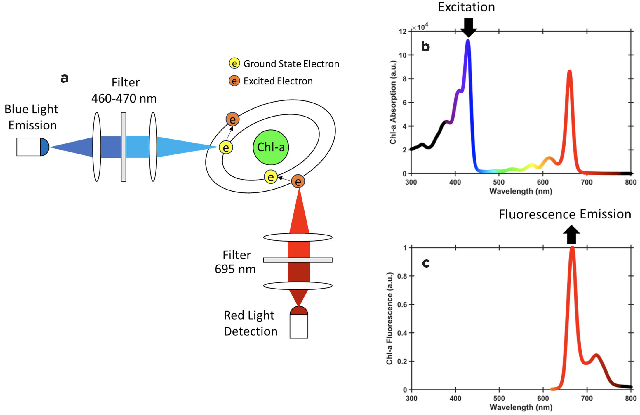
Chl-a molecules fluoresce in the red wavelengths (695 nm) due to higher absorption of light by Chl-a at the 460–470 nm (blue) wavelength (Figure 1, Ocean Optics Web Book). Therefore, Chl-a concentration can be quantified by measuring the emitted fluorescence, with the intensity of the fluorescence signal being proportional to the concentration of Chl-a pigment. The fluorescence intensity is first measured in volts (V) by the fluorometer and then converted into Chl-a concentration using a set of coefficients from calibrations performed by the manufacturer. Given the sensitivity of fluorescence to ambient conditions, (e.g., light; Graff et al., 2015), fluorescence may not be a reliable indicator of actual Chl-a concentration.

Digression. A demonstration of these principles can be done with a blue laser (e.g., pointers <$10 online) and a coastal water (or lake, or any phytoplankton-rich water) sample, or even better, with a phytoplankton culture in a test tube. With all human eyes protected from exposure, point the blue laser at the tube in the dark, and the Chl-a molecules present in the phytoplankton will be seen to emit red light through fluorescence. Laser light emission can be harmful to the eyes. Ensure you take precautions to avoid directing the laser beam toward anyone’s eyes. Fluorometers used by oceanographers use exactly the same principle, with a blue light exciting Chl-a present in natural assemblages of phytoplankton and recording the intensity of the red light thus emitted.

 

FIGURE 1. (a) Illustration of the chlorophyll a (Chl-a) fluorescence principle and the functioning of a fluorometer, representing the interactions between the pigment, the light used for excitation, and the sensor used for detection of the emitted red fluorescence. The (b) absorption and (c) fluorescence spectra of Chl-a in diethyl ether (Dixon et al., 2005) are represented. Note the offset between absorption and fluorescence peak wavelengths (EX: 420 nm and EM: 670 nm) in diethyl ether and the wavelengths used by the fluorometer to detect Chl-a fluorescence in vivo in seawater (EX: 460–470 nm and EM: 695 nm). > High res figure

 

Lab Activity

Materials and Skills Needed

The instructions for the lab activities are provided in the online supplementary materials. The data required for the lab activities are also provided in the supplementary materials and are accessible online through open-access databases and portals. To facilitate the activities, open-access templates (OpenDocument Spreadsheet, .ods) are included in the supplementary materials. Additionally, .ods files containing the expected results for each activity are provided to ensure students can complete all tasks, even if they face challenges with specific steps. Instructors will also find png-format figures illustrating each activity in the supplementary materials.

Students need individual computers with internet access and a spreadsheet application, such as OpenOffice Calc (open access) or Microsoft Excel, to complete the activities. They should be comfortable using spreadsheet software and familiar with basic functions like copying and pasting, calculating averages and standard deviations, creating plots, and performing linear regressions.

Instructors should be familiar with concepts in oceanography (e.g., phytoplankton and fluorescence). While experience with deploying oceanographic instruments, such as fluorometers, and analyzing the resulting data can be helpful, it is not required. However, proficiency in data handling and analysis using spreadsheet software is highly recommended, as students may encounter difficulties during the activities that require additional support.

 

Section 1. Accessing and Exploring Sensor-Based Fluorescence and Discrete Chl-a Data

(1.5 hours)

Accessing and working with observational data can be challenging due to material or geographical constraints that limit data availability. Here, we aim to familiarize students with openly accessible oceanographic data and to help them develop skills in analyzing sensor-based fluorescence and discrete Chl-a data collected as part of the Northeast US Shelf Long-Term Ecological Research (NES-LTER) project. Students will work with authentic data and learn quality control procedures, with the goals of acquiring valuable skills and addressing critical questions about data quality assurance and the management of observational datasets.

 

Part 1. Sensor-Based Fluorescence Chl-a Data

GOAL

Access and work with authentic raw underway fluorescence data, followed by preliminary interpretation of these data.

EXPECTED OUTCOMES

Develop familiarity with underway fluorescence data, including the challenges of handling raw datasets and navigating complex formats, such as date/time. Produce figures to interpret general patterns in the data and engage students in critical discussions about the observed trends.

NARRATIVE

Fluorometers that record Chl-a fluorescence are widely used by the scientific community to estimate phytoplankton biomass in water bodies and to investigate the dynamics of phytoplankton communities. Chl-a fluorescence data can be found on many open access databases. Some examples from US-based research programs are the University-National Oceanographic Laboratory System (UNOLS) Rolling Deck to Repository (R2R), the Environmental Data Initiative (EDI), the Ocean Observatories Initiative (OOI), and the Biological & Chemical Oceanography Data Management Office (BCO-DMO).

Here, we use data from six NES-LTER cruises (EN644, EN649, EN655, EN657, EN661, and EN668) on R/V Endeavor. During each cruise, a pump located near the ship’s bow collects water from 5 m below the ocean’s surface through a system of tubing throughout the ship—called an underway system. Such underway systems are present on most oceanographic research vessels. The underway data are recorded along the cruise tracks and include a suite of navigation (e.g., latitude, longitude, speed), meteorological (e.g., wind speed and direction, light intensity), and oceanographic (e.g., temperature, salinity, Chl-a fluorescence) data. On R/V Endeavor, some of the oceanographic data collected are obtained from an underway water flow-through system that includes temperature and salinity sensors, and two fluorometers, a WETLabs ECO-FLRTD and a WETStar fluorometer. Fluorescence is measured and recorded every second along the ship track. The WETLabs ECO-FLRTD reads Chl-a fluorescence by exciting at a wavelength of 460 nm, the WETStar fluorometer excites at 470 nm, and both fluorometers read emissions at 695 nm (Figure 1). The raw fluorescence is recorded in volts (V) and then converted to Chl-a concentration expressed in units of mg m^–3 based on a manufacturer calibration using a scale factor and blanks including pure water and dark counts. Ship-provided raw underway data are publicly available through the R2R data portal. Raw underway fluorescence data are stored within the TSG Sea-Bird SBE-21 datasets, along with other underway data such as temperature, conductivity, salinity (Sosik, 2019, 2020a, 2020b, 2020c, 2021a, 2021b). These raw data can be challenging to access because of their formats (multiple, non-concatenated, .raw files), which are basically text with separations (e.g., commas, but also tabs) between columns, and without column headers. As part of the NES-LTER project, curated 1-min temporal resolution data, including all navigation and meteorological and oceanographic measurements, can be accessed through the NES-LTER REST API in a comma-​separated values (.csv) format that also includes all the column headers. To facilitate access, we provide the underway data as supplemental .csv files for several cruises as downloaded from the NES-LTER REST API at the time this article was written.

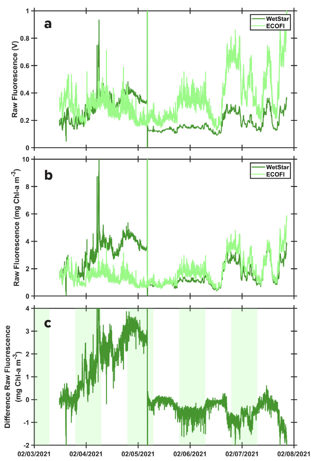
The data show that the two fluorometers recorded slightly different values during each cruise but generally followed a similar pattern (Figure 2 and in online supplementary materials). During the winter 2021 (February) EN661 NES-LTER cruise, the WetStar fluorometer was malfunctioning during the first two days of the cruise, as indicated by the major differences observed when comparing the two fluorometer values (Figure 2). A cleaning of the WetStar fluorometer was performed during the cruise once the problem was identified, resulting in a better match of the sensors afterward. We included these data here because such technical problems occur frequently and highlight the importance of cleaning oceanographic instruments before each deployment, and also the importance of real-time monitoring of the sensors’ displays during a cruise. The difference between the two fluorometers appears to follow a diel cycle (Figure 2c and in online supplementary materials), with a larger difference during daylight hours, highlighting the fact that instruments measuring the same parameters can produce different data and that those deviations can be modified by external influences. This diel pattern might be linked to non-photochemical quenching of Chl-a molecules during the daytime (Marra, 1998; Xing et al., 2012), when light intensity is high, with one of the instruments being more sensitive than the other to this process.

 

FIGURE 2. Examples of (a) underway raw fluorescence (in volts, V), and (b) manufacturer calibrated fluorescence (mg Chl-a m–3) recorded by the WetStar (dark green) and the ECOFl (light green) fluorometers vs. time during the EN661 Northeast US Shelf Long-Term Ecological Research (NES-LTER) cruise in winter 2021. (c) Difference of the manufacturer-​calibrated fluorescence signals between the two fluorometers (mg Chl-a m–3), with light green shaded area representing nighttime (here defined from 7 p.m. to 7 a.m. local time). > High res figure

 

Part 2. Discrete Data for Extracted Chl-a

GOAL

Access and analyze authentic discrete Chl-a data, followed by preliminary interpretation. Gain familiarity with the dataset required for Section 2 of this lab activity.

EXPECTED OUTCOMES

Build an understanding of discrete Chl-a data, including how they are collected, the uncertainties associated with discrete sampling, and the quality control procedures applied. Conduct basic statistical analyses (e.g., averages, standard deviations) and interpret the resulting data.

NARRATIVE

Discrete Chl-a data have historically been collected during oceanographic cruises, primarily from water sampled throughout the water column using Niskin bottles mounted on a CTD-Rosette. The general procedure for discrete Chl-a measurements involves filtering a known volume of seawater to retain all phytoplankton cells on the filter, extracting the Chl-a retained on the filter with a solvent, and then quantifying the amount of Chl-a in the solvent by fluorescence. Additionally, high-performance liquid chromatography (HPLC) can be used to quantify Chl-a concentration. These methods for sampling, filtering, extracting, and quantifying are relatively simple and can be performed as a lab activity, depending on resources available to students.

During NES-LTER cruises, discrete Chl-a samples for the calibration of the underway fluorometers were collected from a spigot connected to the underway system so that the samples contained water that had just run through the two fluorometers (Menden-Deuer et al., 2022). Additional discrete Chl-a samples are routinely collected from the Niskin bottles mounted on the CTD-Rosette at each sampling station at various depths (Sosik et al., 2023), including at the surface (3–7 m depth). While these additional data could be used to post-calibrate the underway fluorometers, we will focus here only on the discrete underway Chl-a data. Before collection, the date and time of sampling were recorded along with the current fluorometer readings. Fifteen to 20 samples were collected on a random timeline during the cruise, while ensuring collection of half the samples during the day and about half during the night, to capture the effects of nonphotochemical quenching (Marra, 1998; Holm-Hansen et al., 2000). Additional effort was devoted to maximizing the dynamic range of fluorescence and corresponding Chl-a concentrations, based on real-time observations of the underway fluorescence signals (e.g., during periods of unusually low or high fluorescence). A collection container with a volume between 500 mL and 1 L was rinsed three times with underway water, then filled. Three plastic 152 mL bottles were then filled to the top with the underway water in triplicates. Immediately after collection, the entire volume of each triplicate was filtered onto Whatman GF/F 25 mm filters using gentle vacuum (not exceeding 150 mm Hg) in a light-limited environment to avoid any degradation of the Chl-a pigments. The filters were then each placed in glass tubes containing 6 mL of 95% ethanol, capped, and stored in the dark at room temperature to extract the Chl-a for approximately 12 hours (±2 hours). After the extraction period, the fluorescence of the samples was recorded with a Turner 10AU fluorometer first as is, and then with the addition of acid to correct for phaeopigments (Wasmund et al., 2006). The discrete underway sample data were digitized and organized, then Chl-a concentration, in mg m^–3 (= μg L^–1), was calculated using coefficients obtained from the in-lab fluorometer’s calibration; this was performed before each cruise based on pure Chl-a standards (Sigma-Aldrich, from Anacystis nidulans algae). Each data point was then given a quality flag based on the IODE (International Oceanographic Data and Information Exchange) quality flag scheme (IOC, 2013) so that only the highest quality data would be included in the post-calibration. Discrete underway Chl-a data from six NES-LTER cruises are available on the EDI data portal (Menden-Deuer et al., 2022).

 

Section 2. Using Discrete Chl-a to Post-Calibrate Sensor-Based Fluorescence

(1.5 hours)

There can be substantial differences between manufacturer-​calibrated continuous fluorescence data and discrete Chl-a concentrations. Manufacturer-calibrated fluorescence values converted to Chl-a concentrations (mg m^–³) should be interpreted with caution because the calibration is typically performed using either pure Chl-a extracts or single-species phytoplankton cultures that may not accurately reflect the local phytoplankton community, environmental conditions (e.g., temperature), or optical properties encountered in the field. Factors such as species composition, physiological state, light history, and colored dissolved organic matter (CDOM) can all influence the fluorescence signal independent of actual Chl-a concentration. The optical components of the fluorescence sensor may also be biofouled during deployment. Although this is minimized by cleaning the sensors before and after each deployment and by maintaining a high flow rate, any biofouling can still alter the recorded optical signal. As a result, without cross-validation, these manufacturer-derived values can be substantially different from in situ Chl-a. Therefore, it is crucial to acknowledge, correct for, and interpret the uncertainty and imprecision in in vivo fluorescence data to interpret the fluorescence signal (Cullen, 1982; Falkowski and Kiefer, 1985; Xing et al., 2017). To obtain reliable, accurate, high-resolution Chl-a data from in vivo fluorescence, the continuous fluorometer data must undergo post-​calibration against discrete Chl-a values. The steps required for this data management are the subject of this hands-on exercise.

 

Part 1. Plotting Sensor-Based Chl-a Fluorescence vs. Extracted Chl-a Concentrations

GOALS

Linking sensor-based underway chlorophyll-a (Chl-a) fluorescence and discrete Chl-a data. Introduce methods required for post-calibrating sensor-based Chl-a fluorescence data.

EXPECTED OUTCOMES

Develop familiarity with linear regression, including the concepts of slope, intercept, and coefficient of determination. Understand the significance of linear regression results and their application in post-calibrating underway Chl-a fluorescence data.

NARRATIVE

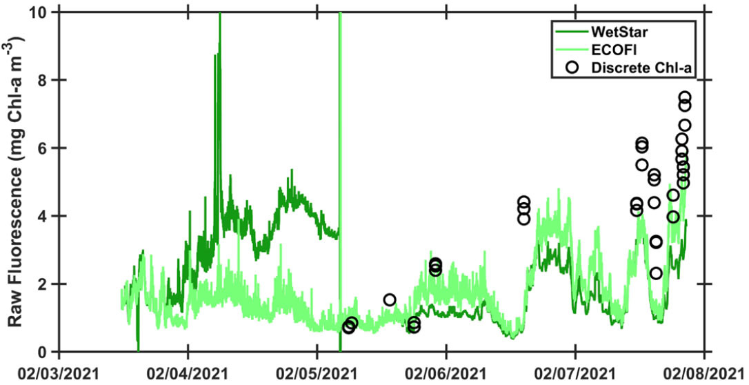
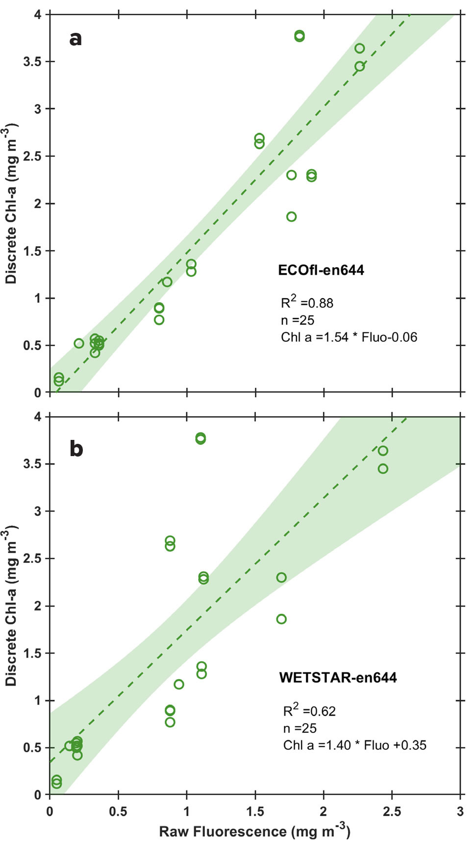
It is now time to compare the discrete Chl-a concentrations with the corresponding underway fluorescence values observed when sampling (Figures 3 and 4). The goal here is to identify whether both fluorometers are equally well suited to use for the post-calibration and to identify the coefficients that will be used for the post-calibration of the fluorometer. Some basic statistical concepts such as linear regression will be introduced. Note that on most oceanographic cruises, only one fluorometer is available to record underway fluorescence, meaning that selection of one of two fluorometers is not possible.

 

FIGURE 3. Raw underway fluorescence (mg Chl-a m–3) during the EN661 NES-LTER transect cruise (February 3 to February 7, 2021, winter in the Northern Hemisphere) from the WetStar (dark green) and the ECO-Fl (light green) fluorometers. The discrete Chl-a concentrations collected in triplicate during the cruise are represented by black dots. Only discrete Chl-a data with an IODE Quality Flag = 1 (good) are shown. Note the change in fluorescence from the WetStar fluorometers on 02/05/2021, which corresponds to the change observed after the cleaning of the instruments. > High res figure

 

FIGURE 4. Discrete Chl-a concentrations (mg m–3) plotted against the matching fluorescence values from (a) the ECO-Fl fluorometer (mg m–3), and (b) the WetStar fluorometer (mg m–3) during the EN644 summer 2019 cruise (August). The green dashes represent the line of best fit from a model I linear regression, with the equation, including the slope and intercept, shown as an insert on each figure. The shaded green area represents the 95% confidence interval obtained for the linear regression model. > High res figure

 

Part 2. Post-Calibration to Estimate Chl-a Concentration from In Vivo Fluorescence

GOALS

Post-calibrate the underway fluorescence data by applying the relationships established in Section 2, Part 1, between the raw fluorescence measurements and the discrete Chl-a concentration data. Compare the raw fluorescence values with the post-calibrated data collected during the three summer cruises and interpret the resulting figures.

EXPECTED OUTCOMES

Gain insight into the significance of post-​calibrating raw fluorescence data for analyzing the inter-​annual variations in phytoplankton biomass within a highly dynamic coastal ecosystem.

NARRATIVE

After identifying the best suited fluorometer, the goal is to apply the relationship obtained from the linear regression to the continuous underway measurements for each cruise (Figure 2 and in online supplementary materials) and ultimately to create a new data package that includes all these post-​calibrated measurements to share with the scientific community. We also present here an illustration of why post-calibration of fluorescence data is essential (Figure 5) and invite the students to interpret the results obtained by comparing post-calibrated fluorescence among three summer NES-LTER cruises.

 

FIGURE 5. (a) Map and bathymetry of summer (in Northern Hemisphere) NES-LTER transect cruises from August 2019 (EN644, green), July 2020 (EN655, light green), and July 2021 (EN668, yellow) from Narragansett Bay, Rhode Island, to the shelf break. (b) Raw underway fluorescence (mg Chl-a m–3) from each cruise vs. latitude (°N; note the reverse x-axis from higher latitudes in the north [left] to lower latitude in the south [right]). (c) Post-calibrated underway fluorescence (mg Chl-a m–3) vs latitude. For clarity, only data from the outbound leg of the transect (north to south) are shown. > High res figure

 

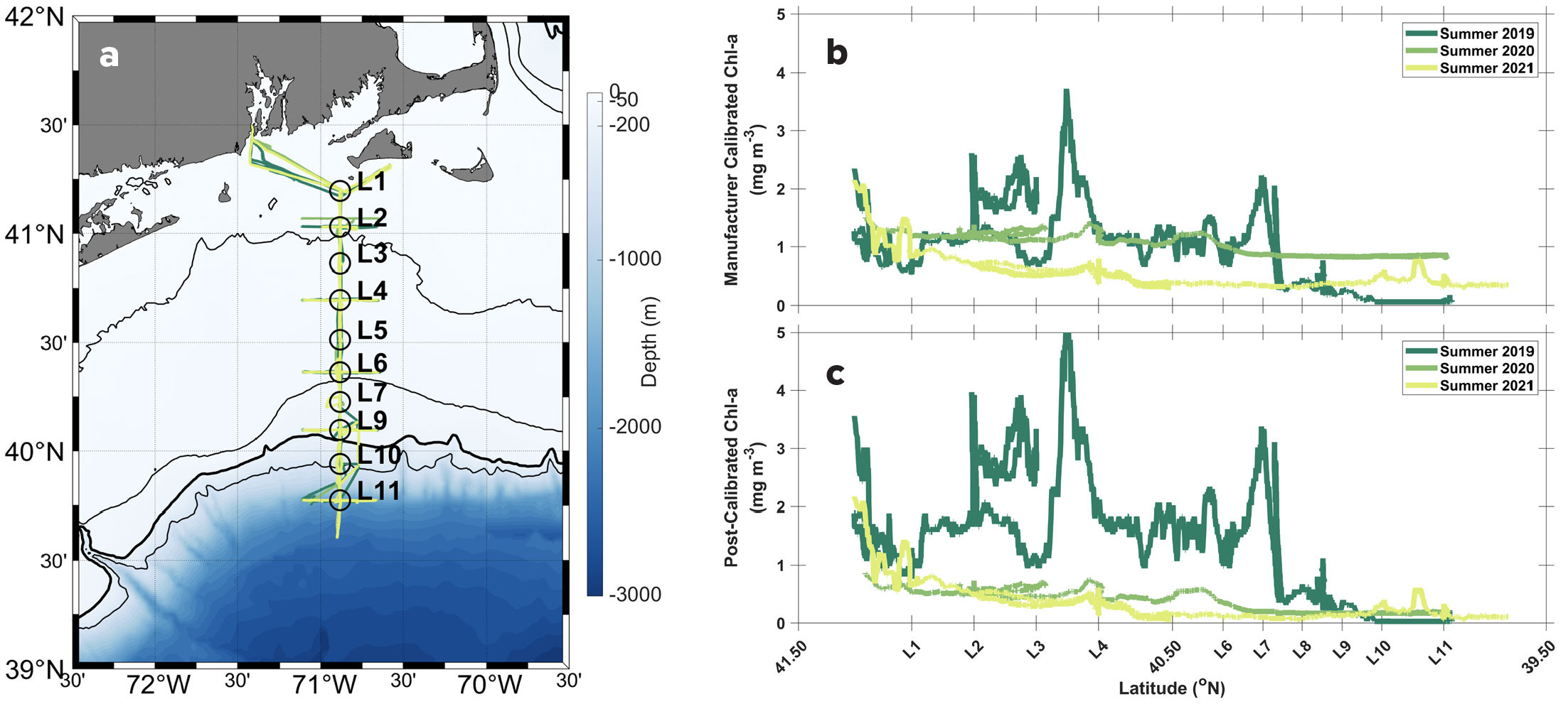
When looking at the data from the three summer NES-LTER cruises together, the first observation is that the fluorescence signal in 2019 has a much higher magnitude and is more variable and “noisy” compared to the signals from the summers of 2020 and 2021. Based on the raw fluorescence values, the concentration of Chl-a was higher, indicating higher phytoplankton biomass in the surface waters of the NES in 2019 than in 2020 and 2021. Additionally, there seemed to be higher concentrations of Chl-a in surface waters along the 2020 transect than in 2021.

The fluorescence signal in 2019 remains more variable and higher than during the other two cruises after post-calibration. Interestingly, while the raw fluorescence data suggested more Chl-a in 2020 than in 2021, post-calibration revealed that the Chl-a concentrations were actually very similar. This underscores the importance of post-calibration when comparing fluorescence values from different cruises.

Some essential background information about the oceanographic context of the NES may be helpful for instructors to interpret the data obtained. To support this, we included an introduction to the seasonal dynamics of the phytoplankton community in NES waters in a dedicated section of the Lab Instructions document, available in the supplementary materials.

Chl-a concentrations were generally higher in inner shelf waters (northern half of the transect) than in the outer shelf waters (southern half of the transect). This difference can be attributed to the shallower depth and greater influence of coastal inputs in the inner shelf region, which result in more nutrients for phytoplankton growth. In contrast, the outer shelf waters are more oligotrophic, similar to some open ocean regions.

During summer, nitrate (an essential nutrient for phytoplankton growth) is completely depleted in the surface waters of the NES, indicating that phytoplankton growth is likely based on remineralized nutrients through the microbial loop, favoring the growth of small phytoplankton cells (Marrec et al., 2021). However, in the summer of 2019, an intense bloom of large diatom cells was observed along the transect. This bloom was comprised of nitrogen-fixing bacteria living in symbiosis with a diatom species (Hemiaulus), providing the necessary nitrogen that was not available as nitrate (Castillo Cieza et al., 2024).

We demonstrated that post-calibrating Chl-a fluorescence values are essential for accurate comparison, as the calibration substantially altered the estimated Chl-a concentrations. In this study, we used fluorescence values from different cruises, where fluorometers either underwent manufacturer calibrations or were replaced by spare instruments of the same model. A similar approach can be applied when comparing fluorescence values from the same study area but obtained from different research vessels or other platforms such as moorings, CTDs, or gliders. Without proper post-calibration, raw Chl-a fluorescence values cannot be reliably compared.

 

Feedback from Students and Recommendation to Instructors

The exercise described here was repeatedly tested with students in class and in self-paced assignments. The major feedback from students was that they struggled with obtaining the data from online repositories in reproducible ways. Different versions of the same spreadsheet tool interpreted dates and number formatting differently. To accommodate these challenges—which could not easily be alleviated as students may have many different software types and settings—we have developed a more explicit step-by-step guide and provided standardized files for each intermediary step, so students can access properly formatted files for each step and can avoid lack of data accessibility or formatting issues. These elements raise awareness for students as they will certainly encounter similar challenges related to data management in their own research or classes. This requirement for troubleshooting often fosters learning and confidence in the gained competency, as students overcome obstacles and find solutions independently. As large-scale open-access databases become increasingly prevalent, the skills developed through this activity are essential and foundational for many researchers.

 

Student Benefits

Our proposed activity offers students a valuable opportunity to better understand the limitations of relying on raw, manufacturer-​calibrated Chl-a values, and more broadly, on any biogeochemical data obtained from sensors. This serves as a general example of working with calibrated instruments. Data users may assume that fluorescence-derived Chl-a concentrations provided by manufacturers represent accurate and true measurements of Chl-a and possibly by extension, biomass. However, as demonstrated in this study, this is not the case.

This exercise shows students critical concepts in data validation and underscores the need for quality control by researchers. This is exemplified by differences between fluorometers with varying specifications that can lead to discrepancies between nighttime and daytime measurements (Figure 2c). These variations suggest that non-photochemical quenching (NPQ) of Chl-a molecules occurs during daylight hours when light intensity is high (Marra, 1998; Xing et al., 2012), with some instruments being more sensitive to this process than others. Ideally, only nighttime fluorescence data should be used for post-​calibration, while daytime values should be corrected for NPQ (Carberry et al., 2019). In our case, we show that the NPQ effect is negligible for our post-calibration. Using discrete data, we show that the relatively high variance in our calibration is likely due to the inclusion of both daytime and nighttime data.

Students also engaged with the importance of clarifying what an instrument measures and what the measurement represents. The concept of C:Chl ratios is fundamental in biomass assessments in oceanographic studies and plays a key role in student learning outcomes by highlighting how data or model estimates are influenced by the conversion factors used. We encourage educators to engage students in discussions on the deep Chl-a maximum (DCM) in oligotrophic waters and the effects of photo­acclimation on cellular Chl-a content. The DCM has often been interpreted in scientific literature and textbooks as a biomass maximum. However, it primarily reflects photoacclimation processes and variations in the C:Chl-a ratio (Mignot et al., 2014; Cullen, 2015; Maranon et al., 2021). This serves as a crucial example of why Chl-a should be used with caution as a proxy for phytoplankton biomass.

Lastly, and this is our central topic, our goal was to empower students with the formal tools of data science, data management, and FAIR practices. A career in data science and management can represent a career pathway in itself or a bridge to other professional opportunities for students. Expertise in data science is highly transferable and can be applied across a wide range of professional fields, within sciences and beyond. A notable example is Amanda Herbst, a coauthor of this study, who after completing a summer internship using the skills covered here, pursued a Master of Environmental Data Science degree at the Bren School of Environmental Science and Management at the University of California, Santa Barbara, and who recently accepted a position as Environmental Analyst for the New England Interstate Water Pollution Control Commission (NEIWPCC) and will be working at the New York State Department of Environmental Conservation.

Students are exposed to the vast universe of freely available data and how to handle them. When sourced from data portals with rigorous quality control procedures and well-documented metadata, these datasets can be valuable resources for research and analyses at minimal cost. Many students, researchers, and institutions face financial constraints when conducting field studies, which often require expensive platforms (e.g., research vessels) and instrumentation (e.g., biogeochemical sensors). By increasing awareness of existing high-quality, open-access datasets, the oceanographic community could make significant advancements. In fact, some long-term observational datasets remain underutilized despite being collected, processed, and stored following state-of-the-art standards (e.g., NSF Dear Colleague Letters 2024). Leveraging these resources could greatly enhance our understanding of oceanographic processes.

 

Concluding Remarks

The main goal of this contribution to Oceanography’s Ocean Education article category is to emphasize to students the importance of proper handling and sharing of post-calibrated data by publishing it in open-access data portals. All the data used in this hands-on activity are openly available, allowing researchers worldwide to access and utilize them. However, as demonstrated, interpreting raw Chl-a fluorescence has limitations. Therefore, providing the scientific community with high-quality post-calibrated Chl-a fluorescence data is essential for advancing research.

An important aspect of sharing high-quality data in open-​access repositories is to include all information necessary for understanding how the data were acquired and analyzed. This additional information, known as metadata, includes intelligible and descriptive data product names, precise temporal and spatial coverage, accurate and complete lists of science keywords, and concise yet readable descriptions of the data products. Instrument calibration documentation (e.g., manufacturer calibration) and data analysis workflows are also crucial metadata components. Publishing open-access data packages following FAIR principles ensures that the science is open, transparent, accessible, inclusive, and reproducible (Wilkinson et al., 2016).

In our case, we created an EDI data package that compiles post-calibrated underway fluorescence data for six NES-LTER cruises, spanning from summer 2019 to summer 2021, as part of coauthor Amanda Herbst’s summer 2021 REU project. The REU research project included all aspects of the research this exercise drew on, including cruise participation to acquire calibration data. The NES-LTER Information Management team supported us in the creation of this data package (Menden-Deuer et al., 2022). Essential steps in creating a data package include a clear description of the methods used to process the data, data quality checks, and additional metadata to improve findability. These steps benefited greatly from the experience of data managers, who play an essential role in modern research projects. Please note that publishing the data package is not included in this activity, as all sample data are already published, and multiple publications of the same data package are not desirable.

 

Acknowledgments

This work was supported by awards from the National Science Foundation (NES-LTER Phase 1: OCE-1655686, NES-LTER Phase 2: OCE-2322676). AH was supported by a Summer Undergraduate Research Fellowship in Oceanography (SURFO; National Science Foundation REU grant # OCE- 1757572). Support through the NASA campaign EXport Processes in the global Ocean from RemoTe Sensing (EXPORTS; grant 80NSSC17K0716) is acknowledged. We thank the students, staff and PIs of the NES-LTER project for their support, and the leadership of Heidi Sosik (Woods Hole Oceanographic Institution). We thank the captains Armanetti, Beuth, and Carty, the R/V Endeavor Crew, and the work of the marine technicians at the University of Rhode Island. Brian Heikes, David Smith, and Jamie Buck are acknowledged for all the effort they put into the SURFO program. We appreciated the enthusiasm and effort of the University of Rhode Island students in the Graduate School of Oceanography class OCG561 (2024), who tested this lab activity and substantively improved the final product.

Marrec, P., A. Herbst, S.E. Beaulieu, and S. Menden-Deuer. 2025. Hands-on post-calibration of in vivo fluorescence using open access data: A guided journey from fluorescence to phytoplankton biomass. Oceanography 38(2):73–82, https://doi.org/10.5670/oceanog.2025.314.

> Supplementary Materials (21.9 MB zipped folder)

1. Carberry, L., C. Roesler, and S. Drapeau. 2019. Correcting in situ chlorophyll fluorescence time-series observations for nonphotochemical quenching and tidal variability reveals nonconservative phytoplankton variability in coastal waters. Limnology & Oceanography: Methods 17:462–473, https://doi.org/10.1002/lom3.10325.
2. Cullen, J.J. 1982. The deep chlorophyll maximum: Comparing vertical profiles of chlorophyll a. Canadian Journal of Fisheries and Aquatic Sciences 39(5):791–803, https://doi.org/10.1139/f82-108.
3. Cullen, J.J. 2015. Subsurface chlorophyll maximum layers: Enduring enigma or mystery solved? Annual Review of Marine Science 7:207–239, https://doi.org/​10.1146/annurev-marine-010213-135111.
4. Castillo Cieza, S.A., R.H.R. Stanley, P. Marrec, D.N. Fontaine, E.T. Crockford, D.J. McGillicuddy Jr., A. Mehta, S. Menden-Deuer, E.E. Peacock, T.A. Ryenearson, and others. 2024. Unusual Hemiaulus bloom influences ocean productivity in Northeastern US Shelf waters. Biogeosciences 21:1,235–1,257, https://doi.org/​10.5194/bg-21-1235-2024.
5. Dixon, J.M., M. Taniguchi, and J.S. Lindsey. 2005. PhotochemCAD 2: A refined program with accompanying spectral databases for photochemical calculations. Photochemistry and Photobiology 81:212–213, https://doi.org/​10.1111/​j.1751-1097.2005.tb01544.x.
6. Falkowski, P., and D.A. Kiefer. 1985. Chlorophyll a fluorescence in phytoplankton: Relationship to photosynthesis and biomass. Journal of Plankton Research 7(5):715–731, https://doi.org/10.1093/plankt/7.5.715.
7. Geider, R.J. 1987. Light and temperature dependence of the carbon to chlorophyll a ratio in microalgae and cyanobacteria: Implications for physiology and growth of phytoplankton. New Phytologist 106(1):1–34, https://doi.org/​10.1111/j.1469-8137.​1987.tb04788.x.
8. Graff, J.R., T.K. Westberry, A.J. Milligan, M.B. Brown, G. Dall’Olmo, V. van Dongen-Vogels, K.M. Reifel, and M.J. Behrenfeld. 2015. Analytical phytoplankton carbon measurements spanning diverse ecosystems. Deep Sea Research Part I 102:16–25, https://doi.org/10.1016/j.dsr.2015.04.006.
9. Holm-Hansen, O., A.F. Amos, and C.D. Hewes. 2000. Reliability of estimating chlorophyll a concentrations in Antarctic waters by measurement of in situ chlorophyll a fluorescence. Marine Ecology Progress Series 196:103–110, https://doi.org/​10.3354/meps196103.
10. IOC (Intergovernmental Oceanographic Commission of UNESCO). 2013. Ocean Data Standards Volume 3: Recommendation for a Quality Flag Scheme for the Exchange of Oceanographic and Marine Meteorological Data. Version 1, IOC Manuals and Guides, 54, Vol. 3., 12 pp., UNESCO, Paris, https://www.ioccp.org/images/D4standards/IOC-OceanDataStandards54-3-2013.pdf.
11. Jakobsen, H.H., and S. Markager. 2016. Carbon-to-chlorophyll ratio for phytoplankton in temperate coastal waters: Seasonal patterns and relationship to nutrients. Limnology and Oceanography 61(5):1,853–1,868, https://doi.org/10.1002/lno.10338.
12. Kaiser, J., and J. Brainard. 2023. Ready, set, share! Science 379(6630):322–325, https://doi.org/10.1126/science.adg8142.
13. Marañón, E., F. Van Wambeke, J. Uitz, E.S. Boss, C. Dimier, J. Dinasquet, A. Engel, N. Haëntjens, M. Pérez-Lorenzo, V. Taillandier, and B. Zäncker. 2021. Deep maxima of phytoplankton biomass, primary production and bacterial production in the Mediterranean Sea. Biogeosciences 18:1,749–1,767, https://doi.org/10.5194/bg-18-1749-2021.
14. Marra, J. 1998. Analysis of diel variability in chlorophyll fluorescence. Oceanographic Literature Review 4(45):617.
15. Marrec, P., H. McNair, G. Franzè, F. Morison, J.P. Strock, and S. Menden-Deuer. 2021. Seasonal variability in planktonic food web structure and function of the Northeast U.S. Shelf. Limnology & Oceanography 66:1,440–1,458, https://doi.org/​10.1002/lno.11696.
16. Menden-Deuer, S., P. Marrec, and A. Herbst. 2022. Underway discrete chlorophyll and post-calibrated underway fluorometer data during NES-LTER Transect cruises, ongoing since 2019 ver 1. Environmental Data Initiative, https://doi.org/10.6073/pasta/16c8e5937a860c882b524fda73408baf (accessed 2024-08-14).
17. Mignot, A., H. Claustre, J. Uitz, A. Poteau, F. D’Ortenzio, and X. Xing. 2014. Understanding the seasonal dynamics of phytoplankton biomass and the deep chlorophyll maximum in oligotrophic environments: A Bio-Argo float investigation. Global Biogeochemical Cycles 28(8):856–876, https://doi.org/​10.1002/2013GB004781.
18. Palevsky, H.I., S. Clayton, H. Benway, M. Maheigan, D. Atamanchuk, R. Battisti, J. Batryn, A. Bourbonnais, E.M. Briggs, F. Carvalho, and others. 2024. A model for community-driven development of best practices: The Ocean Observatories Initiative Biogeochemical Sensor Data Best Practices and User Guide. Frontiers in Marine Sciences 11:1358591, https://doi.org/10.3389/fmars.2024.1358591.
19. Smyth, T., D. Moffat, G. Tarran, S. Sathyendranath, F. Ribalet, and J. Casey. 2023. Determining drivers of phytoplankton carbon to chlorophyll ratio at Atlantic Basin scale. Frontiers in Marine Science 10:1191216, https://doi.org/10.3389/fmars.2023.1191216.
20. Sosik, H. 2019. TSG (SeaBird SBE-21) data as collected during the cruise EN644, NES-LTER. Rolling Deck to Repository (R2R), https://doi.org/10.7284/133997 (accessed 2024-08-23).
21. Sosik, H. 2020a. TSG (SeaBird SBE-21) data as collected during the cruise EN649, NES-LTER # 4. Rolling Deck to Repository (R2R), https://doi.org/10.7284/140244 (accessed 2024-08-23).
22. Sosik, H. 2020b. TSG (SeaBird SBE-21) data as collected during the cruise EN655, NES-LTER. Rolling Deck to Repository (R2R), https://doi.org/10.7284/140353 (accessed 2024-08-23).
23. Sosik, H. 2020c. TSG (SeaBird SBE-21) data as collected during the cruise EN657, NES-LTER transect #7. Rolling Deck to Repository (R2R), https://doi.org/​10.7284/141686 (accessed 2024-08-23).
24. Sosik, H. 2021a. TSG (SeaBird SBE-21) data as collected during the cruise EN661, NES-LTER transect #8. Rolling Deck to Repository (R2R), https://doi.org/​10.7284/146047 (accessed 2024-08-23).
25. Sosik, H. 2021b. TSG (SeaBird SBE-21) data as collected during the cruise EN668, NES-LTER transect #9. Rolling Deck to Repository (R2R), https://doi.org/​10.7284/146138 (accessed 2024-08-23).
26. Sosik, H.M., E.T. Crockford, E. Peacock, T. Rynearson, D. Fontaine, S. Menden-Deuer, P. Marrec, and OOI CGSN Data Team. 2023. Size-fractionated chlorophyll from water column bottle samples collected during NES-LTER Transect cruises, ongoing since 2017. ver 2. Environmental Data Initiative, https://doi.org/10.6073/pasta/a8170b4f30fec183592ea7868d7bc1d4 (accessed 2024-08-23).
27. Stoer, A.C., and K. Fennel. 2024. Carbon-centric dynamics of Earth’s marine phytoplankton. Proceedings of the National Academy of Sciences of the United States of America 121(45):e2405354121, https://doi.org/10.1073/pnas.2405354121.
28. Wasmund, N., I., Topp, and D. Schories. 2006. Optimising the storage and extraction of chlorophyll samples. Oceanologia 48(1).
29. Wilkinson, M.D., M. Dumontier, I.J. Aalbersberg, G. Appleton, M. Axton, A. Baak, N. Blomberg, J.W. Boiten, L.B. da Silva Santos, P.E. Bourne, and J. Bouwman. 2016. The FAIR Guiding Principles for scientific data management and stewardship. Scientific Data 3(1):1–9, https://doi.org/10.1038/sdata.2016.18.
30. Xing, X., H. Claustre, S. Blain, F. d’Ortenzio, D. Antoine, J. Ras, and C. Guinet. 2012. Quenching correction for in vivo chlorophyll fluorescence acquired by autonomous platforms: A case study with instrumented elephant seals in the Kerguelen region (Southern Ocean). Limnology and Oceanography: Methods 10(7):483–495, https://doi.org/10.4319/lom.2012.10.483.
31. Xing, X., H. Claustre, E. Boss, C. Roesler, E. Organelli, A. Poteau, M. Barbieux, and F. d’Ortenzio. 2017. Correction of profiles of in-situ chlorophyll fluorometry for the contribution of fluorescence originating from non-algal matter. Limnology and Oceanography: Methods 15(1):80–93, https://doi.org/10.1002/lom3.10144.

This is an open access article made available under the terms of the Creative Commons Attribution 4.0 International License (https://creativecommons.org/licenses/by/4.0/), which permits use, sharing, adaptation, distribution, and reproduction in any medium or format as long as users cite the materials appropriately, provide a link to the Creative Commons license, and indicate the changes that were made to the original content. Images, animations, videos, or other third-party material used in articles are included in the Creative Commons license unless indicated otherwise in a credit line to the material. If the material is not included in the article’s Creative Commons license, users will need to obtain permission directly from the license holder to reproduce the material.