Introduction
The Arctic has warmed at nearly four times the global average since 1979 (Rantanen et al., 2022), driving widespread changes across the regional Earth system (Box et al., 2019). One key component is the Greenland Ice Sheet (GrIS), the largest freshwater reservoir in the Northern Hemisphere. Satellite observations show significant mass loss in the ice sheet since the late 1990s (Otosaka et al., 2023). This loss supplies freshwater to the North Atlantic in two forms: liquid meltwater from surface and submarine melting, and solid ice discharged as icebergs. In addition to raising global sea level, this freshwater input can alter ocean circulation and stratification (i.e., the vertical layering of the water column).
In the subpolar North Atlantic and Nordic Seas, warm surface waters originating from lower latitudes lose heat to the atmosphere and, as a result, their density increases. Where stratification is already weak, this densification can become strong enough to remove upper ocean stratification entirely, producing a nearly uniform water column in temperature and salinity down to depths of about 1,000 m. This process is known as “deep convection.” When the resulting water mass becomes sufficiently dense to sink, and subsequently spreads horizontally below the unstratified surface layer, the broader transformation is often referred to as “deep water formation,” describing the end state in which water becomes neutrally buoyant at depths of roughly 500–5,000 m. These dense waters feed the lower limb of the Atlantic Meridional Overturning Circulation (AMOC), a major component of global ocean circulation that redistributes heat, freshwater, and other tracers, thereby influencing global climate.
Freshwater from the GrIS may affect the strength of the AMOC. Because freshwater is less dense than seawater, an increase in freshwater input may enhance stratification and suppress deep convection and deep water formation. Consequently, less water would be fed into the lower limb of the AMOC, weakening its circulation. For this reason, AMOC weakening is often projected under scenarios of increased Greenland Ice Sheet melting in a warming climate. This GrIS-AMOC connection is supported by numerous modeling studies of varying complexity that apply freshwater flux anomalies either directly around Greenland or more broadly across latitude bands in the North Atlantic in so-called “hosing experiments” (i.e., idealized simulations in which freshwater is artificially added to the ocean to test circulation sensitivity). However, the pathway from ice sheet discharge to AMOC response involves a complex chain of processes that we discuss in this review.
Observational evidence from paleoclimate records indicates that major weakening of the AMOC on millennial timescales occurred during periods of cold climate. However, increased freshwater input into the North Atlantic appears to have coincided more closely with phases of subsequent AMOC recovery and climatic warming, rather than with the initial weakening itself, a discrepancy often referred to as the “meltwater paradox” (see Hines et al., 2025, for a review). In more recent and less extreme events, such as the Great Salinity Anomaly of the 1960s, the increased input of freshwater from the Beaufort Gyre in the Arctic Ocean (Dickson et al., 1988; Curry and Mauritzen, 2005) is thought to have suppressed deep convection in the Labrador Sea, where mixed-layer depths reached only about 200 m compared to the typical 1,000 m or more (Lazier, 1980). A disruption of the AMOC today would lead to substantial shifts in the climate system, with major impacts on Northern Hemisphere weather patterns, making it a topic of major societal relevance (van Westen and Baatsen, 2025). However, the precise effect of ongoing and future Greenland meltwater pathways and input on the AMOC remains an area of active research and debate within the scientific community (Arrigo et al., 2017; Bower et al., 2019; L.C. Jackson et al., 2019; Little et al., 2019; Moffa-Sánchez et al., 2019; Weijer et al., 2019; R. Zhang et al., 2019; Hirschi et al., 2020; McCarthy et al., 2020; Srokosz et al., 2021).
The AMOC has been continuously monitored since 2004 by the RAPID/MOCHA/WBTS array at 26.5°N and since 2014 by the Overturning in the Subpolar North Atlantic Program (OSNAP) array spanning 53°–60°N. These observational networks have provided invaluable data, revealing significant seasonal to interannual variability in AMOC strength but no discernible long-term trend so far (L.C. Jackson et al., 2022). Future projections of the effect of GrIS melt on the AMOC are often based on hosing experiments, which complement AMOC projections of the Climate Model Intercomparison Project (CMIP) that lack a realistic feedback from GrIS under global warming (Weijer et al., 2020; Drijfhout et al., 2025). A recent study investigating the addition of projected GrIS meltwater to climate simulations found a small, but significant, effect on AMOC slowdown (Mehling et al., 2026). While hosing experiments provide useful insights, their results show markedly different behaviors (Dukhovskoy et al., 2016; L.C. Jackson et al., 2023). They also involve a large number of assumptions and do not fully capture the complexities of how meltwater from Greenland actually leaves the fjords, spreads across shelves, and enters the wider North Atlantic (Figure 1). The influence of these local processes on freshwater fate, and the associated uncertainties in contemporary modeling approaches used to predict the impact of GrIS meltwater on the AMOC, is the topic of this review.
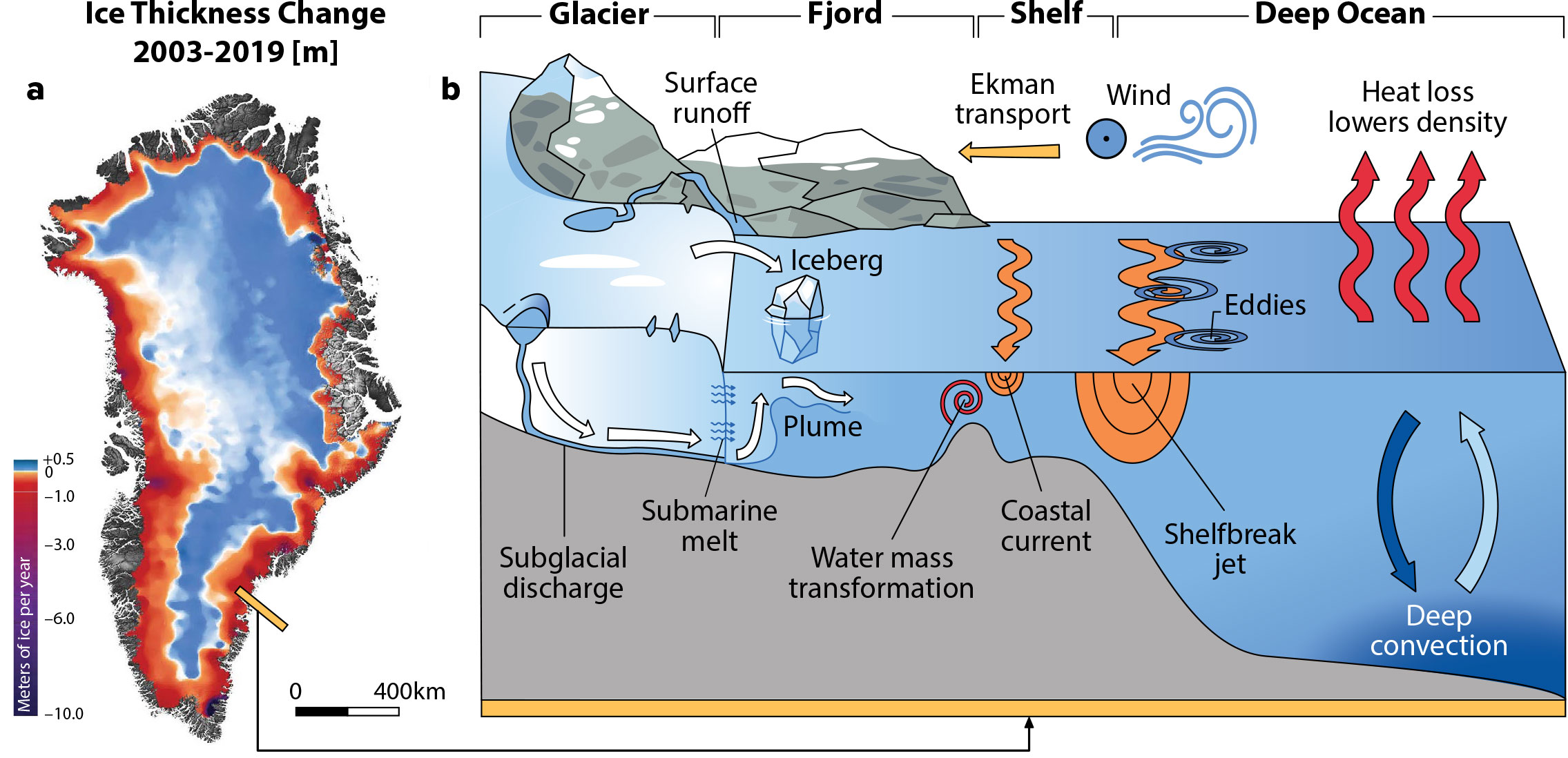
FIGURE 1. (a) Spatial distribution of Greenland Ice Sheet (GrIS) thickness change between 2003 and 2019, reproduced from Smith et al. (2020). (b) A schematic shows the processes influencing the pathway and fate of GrIS meltwater. Certain graphic assets were adapted from VectorMine/Adobe Stock. > High res figure
|
We begin with GrIS ice sheet mass loss and then discuss pathways taken by resulting freshwater in glacial fjords, across the continental shelves, and into the open North Atlantic, also including effects of melting icebergs. For each subsystem, we summarize governing physics and processes controlling GrIS freshwater pathways and identify key knowledge gaps. We also describe how these processes are represented in models, including key assumptions and uncertainties, and outline efforts to reduce them.
How Much Freshwater is Released from the GrIS?
Reconstructions based on reanalyses suggest that the GrIS was close to mass balance from 1960 to 1990 (van Den Broeke et al., 2016, their Figure 2). Since 1992, satellite altimetry has provided measurements of its volume change, together with estimates of inputs from snowfall and outputs from surface melt and ice dynamics (Otosaka et al., 2023). These approaches have been complemented since 2002 by satellite gravimetry from the Gravity Recovery and Climate Experiment (GRACE), which directly observes mass change (Figure 1). For the ice sheet to be in balance, snowfall inputs must equal losses through surface meltwater runoff (hereafter runoff) and ice discharge at the grounding line of marine terminating glaciers. Before 1990, the mean mass turnover, corresponding to the freshwater flux entering the ocean, was 815 ± 72 km3 yr–1, or 0.026 ± 0.002 Sverdrup (Sv, 1 Sv = 106 m3 s–1), representing an approximate equilibrium value. Since the late 1990s, however, the ice sheet has been increasingly out of balance and losing mass, implying a higher freshwater flux. Although there is strong interannual variability (Figure 2a), multi-year averages show a steady increase over roughly 13 years, remaining above the equilibrium level at least through 2021 (Stokes et al., 2025). By the mid-2010s, annual fluxes frequently exceeded 0.035 Sv (1,100 km3 yr–1), a marked increase relative to late twentieth-century conditions (Bamber et al., 2018). Here, we do not account for changes in calving front position (Greene et al., 2024) or ice shelf thinning for the shelves in northern Greenland (Millan et al., 2023), which add an additional 27 km3 yr–1 or 0.0009 Sv from 1985, and 16 km3 yr–1 or 0.0005 Sv since 2000, respectively, to the trends shown in Figure 2a. There are no data available for the full time series shown in Figure 2a, which represent about 14% of the trend since 2000.
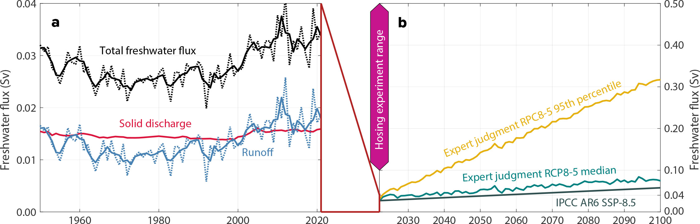
FIGURE 2. (a) Reconstruction of GrIS freshwater fluxes for 1950–2021 based on downscaled ERA5 reanalysis (black) and satellite-derived solid ice discharge (red). Solid lines show three-year running means; dashed lines indicate annual values, except for discharge, which has low interannual variability. (b) Projected GrIS freshwater fluxes under an RCP8.5-like pathway from a structured expert judgment study (teal: median; gold: 95th percentile). IPCC AR6 SSP5–8.5 projections are shown in dark gray and the typical range used in hosing experiments in magenta. > High res figure
|
Although substantial, the additional freshwater flux of about 0.01 Sv, or 300 km3 yr–1 since 2000 (340 km3 yr–1 if we include the trends in calving front retreat and sub-shelf melt mentioned above) is at least an order of magnitude smaller than the typical additional freshwater forcing of 0.1–0.5 Sv used in hosing experiments (see Introduction and Figure 2; L.C. Jackson and Wood, 2018; van Westen et al., 2024). In addition, these hosing experiments often spread the freshwater over a uniform latitudinal band (e.g., L.C. Jackson et al., 2023) and do not account for the large seasonal cycle in the freshwater flux. Some studies have attempted to address these issues by using estimated GrIS freshwater fluxes. Studies such as Böning et al. (2016), Schiller-Weiss et al. (2023), and Hoshyar et al. (2025) show that under present-day Greenland discharge rates, year-to-year changes in ocean salinity are mainly controlled by processes other than Greenland melt. These include variations in the balances between precipitation and evaporation and melting and freezing of sea ice as well as in wind-driven transport (referred to as Ekman transport) that distributes freshwater across the surface ocean. However, these balances may not hold in the future if melt from the GrIS continues to increase, raising a key question: When, and at what rate of melt, will Greenland freshwater notably affect the AMOC?
The response of the GrIS to future climate has been explored using ice sheet models forced by multiple climate models from the fifth phase of CMIP (CMIP5; Goelzer et al., 2020). These simulations suggest relatively modest increases in freshwater flux over the next century (Figure 2b). Under the most extreme emissions scenario (RCP8.5), the projected anomaly (i.e., the excess freshwater relative to the early 1990s baseline) is about 0.02 Sv. However, these projections do not fully reproduce recent observed changes, and they exhibit a wide spread in model results by 2100 (Aschwanden and Brinkerhoff, 2022). Large uncertainties arise from incomplete physical understanding, limited observations of key boundary conditions, and the complex coupling between fjord-scale ocean processes and marine-terminating glaciers, for example, the effect of warm Atlantic Water on the melting of glacier fronts (Grist et al., 2014; Wood et al., 2024). Some potentially important processes, including increased deposition of black carbon and other impurities and changes in subglacial hydrology, are generally not represented in current ice sheet models.
This type of forecasting problem is often described as deep uncertainty (Aspinall, 2010). A useful approach in such cases is structured expert judgment (an approach in which multiple experts systematically assess likely and low-probability outcomes under deep uncertainty; Aspinall, 2010), which has been applied to assess not only the median response but also low-probability, high-impact outcomes under an RCP8.5-like scenario (Bamber et al., 2019). In this framework, an average freshwater flux exceeding 0.2 Sv by 2100 cannot be ruled out (Figure 2; Bamber et al. 2022).
Improvements in the physical representation of processes in ice sheet models are ongoing, but poorly observed and/or constrained boundary conditions will remain a barrier to “conventional” deterministic modeling approaches (Aschwanden et al., 2021), as will the complex small-scale processes at the ice-ocean interface. Nonetheless, longer observational records of ice sheet mass balance and its components, together with advances in computational power, model resolution, and input data, are expected to improve the fidelity of numerical models.
In a broader perspective, the additional 0.01 Sv of Greenland meltwater since the 2000s is only one of several freshwater sources entering the North Atlantic. Another major source is freshwater exported from the Arctic Ocean. Arctic freshwater depends on river discharge, precipitation and evaporation, and exchange through gateway straits (e.g., Haine et al., 2015; Tsubouchi et al., 2024). The mean export of freshwater from the Arctic is around 0.2 Sv (Tsubouchi et al., 2018), with large observational uncertainties associated with the small freshwater transport compared to the total volume transport through the gateways (Le Bras and Timmermans, 2025), as well as the known sensitivity of freshwater transport calculations on the choice of a reference salinity (Schauer and Losch, 2019). Arctic freshwater export varies substantially, particularly through modulation of the Beaufort Gyre. When the Beaufort Gyre spins up under intensified anticyclonic wind forcing, it stores large volumes of low-salinity surface water. When the winds weaken or reverse, this freshwater is rapidly released through Fram Strait and the Canadian Arctic Archipelago. Such releases have been linked to basin-scale events like the Great Salinity Anomaly of the 1970s, associated with an additional 0.06 Sv freshwater export sustained over 10 years (Curry and Mauritzen, 2005) and smaller anomalies in subsequent decades (e.g., J. Zhang et al., 2021). These anomalies propagate through the subpolar North Atlantic, freshening extensive regions and potentially influencing convection and circulation for years. An intensifying hydrological cycle and increasing river discharge into the Arctic further expand the freshwater available for export, much of which has been accumulating in the Beaufort Gyre since the 2000s (Lin et al., 2023; Le Bras and Timmermans, 2025). A future release of this freshwater into the North Atlantic is plausible but remains difficult to predict (Haine et al., 2015; Q. Wang et al., 2024). In comparison, other land-based ice sources, including glacier systems in the Canadian and Russian Arctic and on Svalbard, contribute much smaller freshwater volumes, together supplying an absolute runoff that is roughly eight times lower than that of the GrIS (Bamber et al., 2018, their Figure 3).
In What Form is GrIS Freshwater Entering the Ocean?
GrIS freshwater that enters the ocean in different forms strongly influences subsequent freshwater pathways. Compared to the late twentieth-century baseline, since 2000, about 60% of the additional freshwater input has come from liquid runoff due to surface melting, while the remaining 40% is delivered as solid ice via calving and submarine glacier melt (Figure 2a). The total freshwater flux is highly seasonal, with summer values reaching up to five times the annual mean (Bamber et al., 2018, their Figure 7).
Liquid runoff enters the fjords or coastal ocean either in the surface layer as rivers or streams, or subsurface as subglacial discharge at the grounding line of glaciers. The ratio between surface and subglacial discharge is highly uncertain and likely variable in space and time (Schmidt et al., 2025), but it is important for the fate of the freshwater (see section on Fjord Scale). Additional freshwater is delivered by calving of icebergs, with icebergs either melting within the fjord or transporting freshwater over longer distances (see section on Icebergs), and by submarine melting released along the depth range of the glacier terminus.
Submarine melting at glacier fronts can be estimated from ambient fjord temperature, salinity, and velocity using a three-equation model (see Malyarenko et al., 2020, for a review). These equations include parameters originally developed for floating ice tongues (Scheduikat and Olbers, 1990; Jenkins et al., 2010); their applicability to vertical glacier fronts in Greenland remains debated (R.H. Jackson et al., 2020; Schulz et al., 2022; Cusack et al., 2023; Zhao et al., 2024). How to realistically estimate submarine melt at these vertical fronts is still an open question, and progress is limited by a lack of observational data, in particular, by the difficulty of directly measuring melt rates in the field. Repeated multibeam surveys that track changes in glacier-front position (e.g., Sutherland et al., 2019; Abib et al., 2023) and acoustic tracking of icebergs’ ice–ocean interfaces, combined with co-located measurements of temperature, salinity, and fine-scale velocity (Weiss et al., 2025), offer promising observational approaches. However, even with an idealized melt parameterization, unresolved small-scale features at glacier fronts—for example, undercutting and overcutting, trapped air bubbles or sediment, and poorly constrained fjord-scale velocity, temperature, and salinity fields at the ice–ocean interface—will remain major sources of uncertainty for the foreseeable future. Because the depth at which freshwater enters fjords strongly influences its subsequent pathways and distribution in the ocean (see next section), uncertainties in melt rate parameterizations at the glacier face propagate to larger-scale uncertainties in fjord and ultimately ocean circulation.
How is Freshwater Modified Before Entering the North Atlantic?
Runoff as Surface and Subglacial Discharge
Subglacial discharge released at the glacier base generates buoyant plumes that rise along the ice face while entraining ambient seawater (Figure 1). These plumes control how freshwater is mixed into the ocean, thereby influencing the transformation and export of Greenland meltwater into fjord circulation. As they evolve, plumes pass through distinct regimes: an initial upwelling phase dominated by vertical velocity, a plume-pool phase where vertical motion is converted to horizontal momentum, and a final outflow phase in which waters spread laterally away from the glacier (Mankoff et al., 2016; McConnochie et al., 2020; Ovall et al., 2025). Depending on the magnitude of the subglacial discharge flux, fjord stratification, and plume entrainment, these plumes can reach the surface (e.g., Mankoff et al., 2016) or equilibrate in subsurface waters (e.g., Stevens et al., 2016).
Observations of these stages remain sparse as the near-glacier environment is difficult to access. Most existing measurements capture the plume pool or downstream outflow using autonomous vehicles (e.g., Mankoff et al., 2016; Stevens et al., 2016; R.H. Jackson et al., 2020; Inall et al., 2024), instruments deployed by helicopter or from the glacier surface (e.g., Bendtsen et al., 2015; Podolskiy et al., 2021), or remote sensing (e.g., Schild et al., 2016; Everett et al., 2021). Observations of the upwelling core are rare, limited to measurements by tagged seals (Everett et al., 2018) and recent direct measurements of vertical velocity and plume geometry from an autonomous vessel (Figure 3c; Ovall et al., 2025).
When the plumes detach from the glacier, they are often observed as warm, salty anomalies due to entrainment of deep fjord waters (e.g., Beaird et al., 2018; Cowton et al., 2023). Within tens of meters of the ice face, the discharged freshwater has already mixed extensively with ambient fjord water and reached a salinity of roughly 30 g kg–1 with a dilution ratio of at least 20:1 to 30:1, thus falling between seawater and meltwater (Mankoff et al., 2016; R.H. Jackson et al., 2017). For comparison, in mid-latitude estuaries, freshwater typically transitions from 0 g kg–1 to 30 g kg–1 over kilometers rather than meters. This contrast highlights the efficiency of near-glacier mixing.
In modeling studies, plume dynamics are either explicitly resolved (Figure 3a) or parameterized to capture their bulk behavior (Figure 3b). High-resolution, non-hydrostatic models that resolve the upwelling plume provide insight into how entrainment and melt depend on discharge flux, stratification, and ice slope, but they are computationally expensive and typically limited to domains of tens to hundreds of meters (e.g., Sciascia et al., 2013; Slater et al., 2015; Cusack et al., 2023; Zhao et al., 2024; Ovall et al., 2025). In fjord- and larger-scale models, plumes are usually parameterized using buoyant plume theory, which describes the rise of a buoyant source in a stratified fluid using conservation of mass, momentum, heat, and salt (Jenkins, 2011; Cowton et al., 2015; Hewitt, 2020). Plume theory is typically coupled to the three-equation melt parameterization (see previous section), relating plume velocity and water properties to a melt rate. In such models, the plume scheme is implemented as a boundary condition at the glacier, injecting plume water at neutral buoyancy depth (e.g., Cowton et al., 2015; Wang et al., 2023).
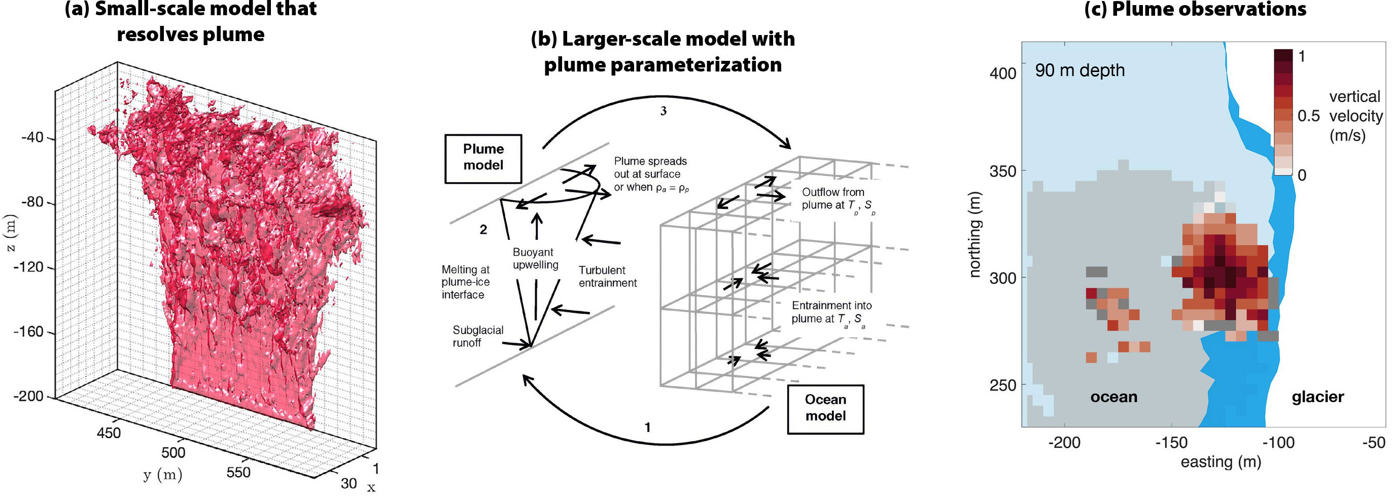
FIGURE 3. (a) Large Eddy Simulation (LES) of a subglacial discharge plume (Zhao et al., 2024), showing the vertical velocity surface, where w = 0.2 m s–1. (b) Schematic of a plume parameterization (Cowton et al., 2015) used to force the boundary of a larger-scale ocean model. (c) Observations of a subglacial discharge plume (Ovall et al., 2025), where vertical velocity is shown on a horizontal slice at 90 m depth. The glacier terminus at this depth is shown in blue. Light gray indicates locations with velocity observations but no plume upwelling, while dark gray indicates plume upwelling where vertical velocity measurements are biased. Light blue indicates regions with no velocity observations. > High res figure
|
Both plume-resolved and plume-parameterized models are sensitive to the poorly constrained spatial distribution of subglacial discharge along the terminus (e.g., Slater et al., 2015). For parameterized plumes, additional uncertainties arise from the empirically prescribed entrainment coefficient and the assumed plume geometry. Most implementations represent the discharge as either a point plume, corresponding to channelized outflow from a single subglacial conduit, or a (truncated) line plume, representing more distributed discharge along the ice face (Jenkins, 1991; Slater et al., 2015, 2017; R.H. Jackson et al., 2017). Recent measurements by Ovall et al. (2025) suggest that a point-plume geometry with an enhanced entrainment coefficient reproduces observations best. Furthermore, plume theory represents only the upwelling phase and does not capture the transition to horizontal outflow and associated mixing, and injecting plume waters into a single vertical grid cell makes results strongly resolution-dependent (Wang et al., 2023). Despite these issues, plume parameterizations remain computationally feasible for fjord- and larger-scale models and are a more realistic representation than prescribing subglacial discharge as a surface freshwater flux.
A large but poorly constrained fraction of GrIS freshwater enters the fjords at the surface. In contrast to subglacial discharge, this freshwater does not drive vigorous mixing and upward transport but rather creates a stable surface stratification (e.g., Stuart-Lee et al., 2021) that influences subsequent freshwater pathways.
Fjord Scale
After rising buoyantly along the ice face in upwelling plumes, subglacial discharge and submarine meltwater leave the glacier as glacially modified water that flows away from the terminus either subsurface at their depths of neutral buoyancy or at the surface (Figure 1). The freshwater export is further transformed by fjord-scale processes such as wind-driven circulation, tides, internal waves, and mixing at sills (Spall et al., 2017; R.H. Jackson et al., 2018; Cusack et al., 2023). Tracing the export and modification of glacial freshwater through fjords remains challenging: many studies infer freshwater pathways from temperature and salinity alone, as these are the most widely available observations (e.g., Mortensen et al., 2020; Muilwijk et al., 2022). However, fjord waters reflect a mixture of multiple freshwater and oceanic sources, so temperature and salinity alone are often insufficient to uniquely separate them. Additional constraints from noble gases can more robustly distinguish freshwater sources and quantify meltwater fractions (Beaird et al., 2015, 2018; Huhn et al., 2021). But even with accurate meltwater concentrations, freshwater export depends not only on concentration but also on velocity. In Sermilik Fjord (East Greenland), noble gas observations show high meltwater fractions in the upper ~200 m that increase toward the surface, but combining these with velocity estimates reveals maximum export near ~100 m depth (Beaird et al., 2018). Robust estimates of freshwater pathways therefore require additional information about current-velocity structures.
While fjord-resolving numerical models have been used to study processes that modify glacial freshwater within fjords (e.g., Slater et al., 2018; Zhao et al., 2023), these processes cannot be resolved in regional or global ocean models, where horizontal resolution is far too coarse to represent fjords explicitly. As a result, Greenland freshwater is typically introduced at the ocean surface in idealized hosing experiments that neglect the strong mixing, entrainment, and redistribution that occur within fjords. This simplification concentrates freshwater at the surface, biasing increases in stratification toward an unrealistically strong and shallow signal, whereas in reality it is distributed more gradually over depth. This bias potentially exaggerates the suppression of deep convection and deep water formation, limiting the realism of simulated responses in ocean circulation.
One alternative for large-scale models is the use of reduced-physics fjord box models that parameterize key processes while remaining computationally efficient. Building on fjord-specific empirical approaches (Muilwijk et al., 2022) and idealized box models (Sanchez et al., 2023), a promising new model proposed by Slater et al. (2025) represents a fjord as multiple vertical layers exchanging heat, salt, and volume, thereby capturing the integrated effects of subglacial discharge, iceberg melting, fjord-shelf exchange, and vertical mixing. Validation against high-resolution fjord simulations shows that this framework reproduces many aspects of seasonal hydrographic evolution, although its response to changes in adjacent shelf water conditions on short time scales remains limited. While simplified and currently omitting processes such as winds, sea ice, and tides, this approach offers a flexible pathway for including fjord-scale freshwater transformation in larger climate and sea-level models. Embedding such reduced-physics fjord representations within larger-scale frameworks (e.g., the Arctic Subpolar Gyre State Estimate; Nguyen et al., 2021) could reduce biases in upper ocean stratification on the shelves and consequently horizontal density gradients that control coastal currents, including the eddy field and exchange between the shelf and the open ocean. Although the direct impact of fjord parameterizations on AMOC simulations is difficult to anticipate within such a complex system, this approach to parameterization provides a promising route toward improving projections of Greenland’s freshwater influence on the North Atlantic.
Fjord-Shelf and Shelf Break
After leaving the fjords, modified meltwater encounters the coastal circulation on the continental shelf (Figure 1). The 200–400 m deep shelves surrounding Greenland are characterized by a narrow coastline-to-shelf transition and a broader shelf-to-basin transition. This bathymetry supports two main current systems. Coastal currents flow within 20–40 km of the shoreline and are maintained by a freshwater wedge trapped against the coast that sets up a horizontal density gradient. Shelf break currents run parallel to the shelf break and are driven by density gradients between lighter shelf waters and denser basin waters. Both current systems are surface intensified, with peak velocities in the coastal current along southern Greenland exceeding 1 m s–1 (Sutherland and Pickart, 2008; Foukal et al., 2020; Duyck and De Jong, 2021), and long-term mean velocities of 0.5–0.6 m s–1 (Le Bras et al., 2018; Pacini et al., 2020). In the shelf break currents, the speeds can reach up to 0.7–0.9 m s–1 (Duyck and De Jong, 2021), with long-term means of 0.4–0.5 m s–1 (Le Bras et al., 2018).
In addition to these currents, which flow primarily along the coastline, winds and cross-shelf canyons drive cross-shelf transport. East of Greenland, downwelling-favorable northerly winds keep the coastal current trapped against the coast from Fram Strait to Cape Farewell (Pennelly et al., 2019; Foukal et al., 2020; Duyck and De Jong, 2021; Schiller-Weiss et al., 2023; Vianco and Foukal, 2025; Pagan et al., 2026), likely retaining most freshwater within the coastal current. Although the structure is only known for a few locations, the wind forcing that drives surface flow toward the coast appears to be balanced by offshore transport at depth (Pickart et al., 2005; Harden et al., 2014). In contrast, west of Greenland, prevailing northwesterly winds favor upwelling that pushes surface waters offshore, enabling exchange between the fresh inshore branches of the West Greenland Coastal Current and the shelf break West Greenland Current, and drawing warmer, saltier offshore water onto the shelf at depth. This east-west contrast in cross-shelf freshwater transport is evident in satellite observations of sea surface salinity (Majumder et al., 2021; Castelao and Medeiros, 2022; Reverdin et al., 2025) and ocean color (Figure 4).
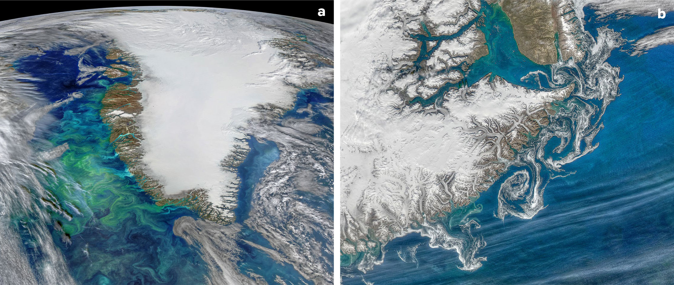
FIGURE 4. Visible-band satellite imagery of Greenland. (a) A MODIS-Aqua image depicts a phytoplankton bloom off the West Greenland shelf (August 29, 2019). In contrast to the green waters in the west, the Southeast Greenland shelf appears relatively blue, reflecting suppressed phytoplankton growth under downwelling conditions. (b) Eddies are apparent in a MODIS-Aqua image of sea ice as the East Greenland Coastal Current flows past Scoresby Sound and the Blosseville Coast (August 14, 2020). Images are from the NASA Ocean Color Image Gallery: (a) https://oceandata.sci.gsfc.nasa.gov/gallery/649/, (b) https://oceandata.sci.gsfc.nasa.gov/gallery/718/. > High res figure
|
Offshore freshwater export is further mediated by eddies generated by flow over rough topography, wind variability, and instabilities associated with the horizontal density gradients between the currents (Harden and Renfrew, 2012; Le Bras et al., 2018; Foukal et al., 2020; Pacini et al., 2020, 2021; Gelderloos et al., 2021; Pacini and Pickart, 2022; Foukal and Pickart 2023; Gou et al., 2023). These eddies act as efficient exchange mechanisms between the shelf and the open ocean by intermittently detaching from boundary currents and transporting shelf waters into the basin interior, while also drawing denser offshore waters back onto the shelf. In doing so, they provide a key pathway for freshwater to leave the constrained coastal current system and enter the broader subpolar gyre circulation. This cross-shelf exchange is particularly important because it controls how much Greenland-derived freshwater can reach regions of deep water formation rather than remaining trapped near the coast. However, eddies exist on spatial scales that are often not resolved in larger-scale models, and their effects on horizontal dispersion must be parameterized, introducing another source of uncertainty. As shown in Figure 5, tracer (and hence freshwater) dispersal varies significantly between two experiments with different horizontal resolutions. In the high-resolution experiment, which resolves many of the eddies formed along the West Greenland Current, significantly more tracer reaches the Labrador Sea interior, stratifying the northern part of that basin.
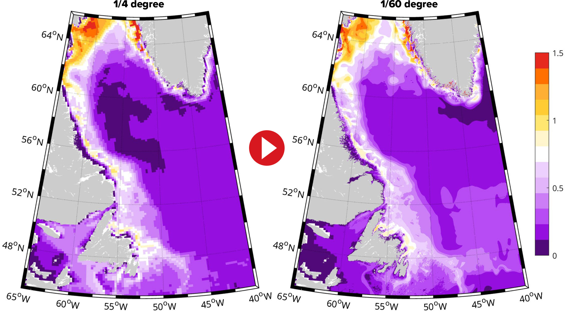
FIGURE 5. Animation of the depth integrated concentration of a Greenland discharge passive tracer (with the amount of tracer added in any grid point and timestep proportional to the amount of liquid discharge input into the model from Greenland, based on Bamber et al. [2018]). (left) 1/4-degree model resolution. (right) 1/60-degree Labrador Sea nesting. See Pennelly and Myers (2020) for further details on the model configurations, experiments, and tracer setup. > High res figure
|
Together, these currents transport Greenland freshwater along and across the shelf, often redistributing it far from its source. The pathways depend on both the location and the depth of entry. For example, freshwater introduced at the surface on the East Greenland shelf can be retained for thousands of kilometers, whereas input on the West Greenland shelf is more readily transferred to the shelf break (Castelao et al., 2023). As a result, water reaching the Labrador Sea along the West Greenland shelf often originates from the East Greenland current system (Myers, 2005; Gillard et al., 2016; Luo et al., 2016). Conceptually, the shelves can be viewed as “leaky conduits,” where freshwater leaves the boundary current system only under specific conditions (Eddy Carmack, Fisheries and Ocean Canada [retired], pers. comm, 2026).
Continuous observations of the current system around Greenland remain sparse and uneven due to icebergs and sea ice, and are complicated by the intermittent and localized nature of cross-shelf transport (e.g., Coquereau et al., 2024). Identifying Greenland meltwater using temperature and salinity is further challenged by other freshwater sources, such as Arctic outflow through Fram Strait, whose variability can produce salinity anomalies comparable to or larger than those from Greenland runoff (Schiller-Weiss et al., 2023). Noble gas tracers provide a more robust alternative (Beaird et al., 2023), but their high cost and limited deployability prevent continuous, large-scale observations. Bulk freshwater flux estimates are often used instead to trace freshwater in observational data (e.g., Bacon et al., 2002; Lin et al., 2018; Håvik and Våge, 2018; Foukal et al., 2020; Foukal and Pickart, 2023; Gou et al., 2023), but they depend on assumptions such as reference salinity (Schauer and Losch, 2019) and current definitions.
Recent advances in high resolution modeling present promising avenues for progress (Böning et al., 2016; Dukhovskoy et al., 2019; Pennelly et al., 2019; Tagklis et al., 2020; Martin and Biastoch, 2023) as they allow unambiguous tracking of Greenland meltwater via passive tracers. Coarse-resolution models tend to underestimate boundary current strength, over-broaden circulation, and fail to resolve most eddies that likely drive cross-shelf exchange (Spall et al., 2024). In contrast, fine-resolution models better represent exchange between shelf and basin, leading to stronger stratification, more localized deep convection, and improved AMOC representation (e.g., Pennelly et al., 2019; Tagklis et al., 2020; Hoshyar et al., 2025). Key sensitivities in these simulations include bathymetry and atmospheric forcing. Realistic shelf exchange depends strongly on accurate seafloor representation and high-quality reanalysis winds (Castelao et al., 2019; Martin and Biastoch, 2023). Recent datasets such as BedMachine (Morlighem et al. 2017) and the Copernicus Arctic Regional Reanalysis (CARRA; Schyberg et al., 2020) improve these constraints, although uncertainties remain. Further progress is expected from coupling ocean models to ice and atmospheric variability, improved data assimilation (Haine et al., 2021), and continued refinement of bathymetry and forcing fields. Progress in any of these areas will help reduce overall uncertainty, although their direct impact on simulated AMOC behavior remains difficult to isolate given the complexity of the system.
Icebergs
The GrIS calves between 200 Gt and 500 Gt of icebergs every year (e.g., Bigg et al., 1997; Rignot et al., 2011; Enderlin et al., 2014; Bamber et al., 2018), corresponding to approximately half of the ice sheet’s annual mass loss (e.g., Figure 2; Enderlin et al., 2014; Bamber et al., 2018). Most icebergs of Greenland origin range in size from 100 m to 500 m, with an upper bound for those in Greenland fjords of around 2 km (Sulak et al., 2017), and they exhibit a wide range of shapes and ratios of width to length, although more recent work assigns iceberg size based on calving front thickness (Abello et al., 2025). While a significant portion (10%–50%) of the icebergs’ mass melts before they reach the open ocean (Enderlin et al., 2016), what remains of an iceberg releases freshwater in the open ocean, away from its sources (Martin and Adcroft, 2010), potentially impacting ocean dynamics (e.g., Cenedese and Straneo, 2023). Fjord-scale modeling studies find that icebergs melt year-round and that they make a crucial contribution to fjord circulation and hydrography (e.g., Davison et al., 2022; Kinne et al., 2025).
The role of icebergs in transporting Greenland freshwater into the interior North Atlantic remains an open question. On the one hand, icebergs may be less important because many remain within boundary currents and are relatively small compared to Antarctic icebergs; on the other hand, they represent a substantial fraction of total freshwater input that, unlike liquid runoff, may more readily escape boundary currents and reach the open ocean without relying on eddy-driven transport. Given the limited observations of iceberg fate in the open ocean, their impact remains uncertain and requires improved representation in models.
Until recently, many ocean models did not include explicit iceberg physics and instead treated all discharge as liquid freshwater. Early iceberg models represented icebergs as drifting particles that melted through processes such as basal and side melting, wave erosion, and atmospheric heat fluxes, including sensible heat exchange and sublimation (Bigg et al.,1997). These frameworks were later extended to include ocean temperature effects and sea ice modulation of wave erosion (Gladstone et al., 2001) and were subsequently coupled to global ocean models (e.g., Marsh et al., 2015; Davison et al., 2020, 2022; Condron and Hill, 2021; Kajanto et al., 2023; Hager et al., 2024; Summers et al., 2025). Further improvements include iceberg fragmentation (Martin and Adcroft, 2010), iceberg interaction with the vertically integrated profiles of ocean velocity and temperature (Rackow et al., 2017; Marson et al., 2018), locking of icebergs in sea ice (Marson et al., 2024), and Eulerian approaches (e.g., Davison et al., 2020; Erokhina and Mikolajewicz, 2024; Summers et al., 2025).
Uncertainties associated with iceberg components in ocean models are twofold. First, formulations of iceberg melt and disintegration by, for example, heat fluxes and wave erosion, are not well constrained by observations, and there are knowledge gaps regarding how icebergs interact with the ocean and the atmosphere. Second, all iceberg models are sensitive to input data and the poorly constrained spatio-temporal calving rates and iceberg geometries. Their responses vary depending on whether they are forced by equal input around Greenland or by point distribution (e.g., Gillard, 2020). In many model applications, icebergs only interact with the ocean surface layer rather than with the ocean at their full depth ranges, and are only points in space (i.e., do not cover ocean area). With few exceptions (Marson et al., 2024), dynamical interaction with sea ice is simplified, with implications for iceberg lifespan and melt location as well as timing. Additionally, except with the newest very high-resolution simulations, the fjords are not well resolved and thus the input locations of the iceberg discharge are likely shifted closer to the fjord mouths and the continental shelf, with uncertain impacts on the simulation. Shapes and sizes of icebergs, and how they drift, melt, and input their freshwater and nutrients into the open ocean, are neither well quantified nor understood. In many studies, including icebergs alters the spatial and temporal distribution of freshwater input in the North Atlantic, but the resulting differences in circulation remain comparable to model internal variability. Ultimately, it remains an open question whether iceberg drift and melt exert a first-order control, or merely a second-order influence, on the distribution and fate of Greenland freshwater in the North Atlantic.
Where Does the Freshwater Go in the North Atlantic?
The ongoing discussion of whether (or when) accelerated GrIS melting will affect large-scale ocean circulation often focuses on the direct impact of freshwater on stratification, particularly in the Labrador Sea, a key region for water mass transformation where a reduction in deep convection could potentially weaken the AMOC. However, this framing does not capture the complexity of the regional circulation system (Figure 6).
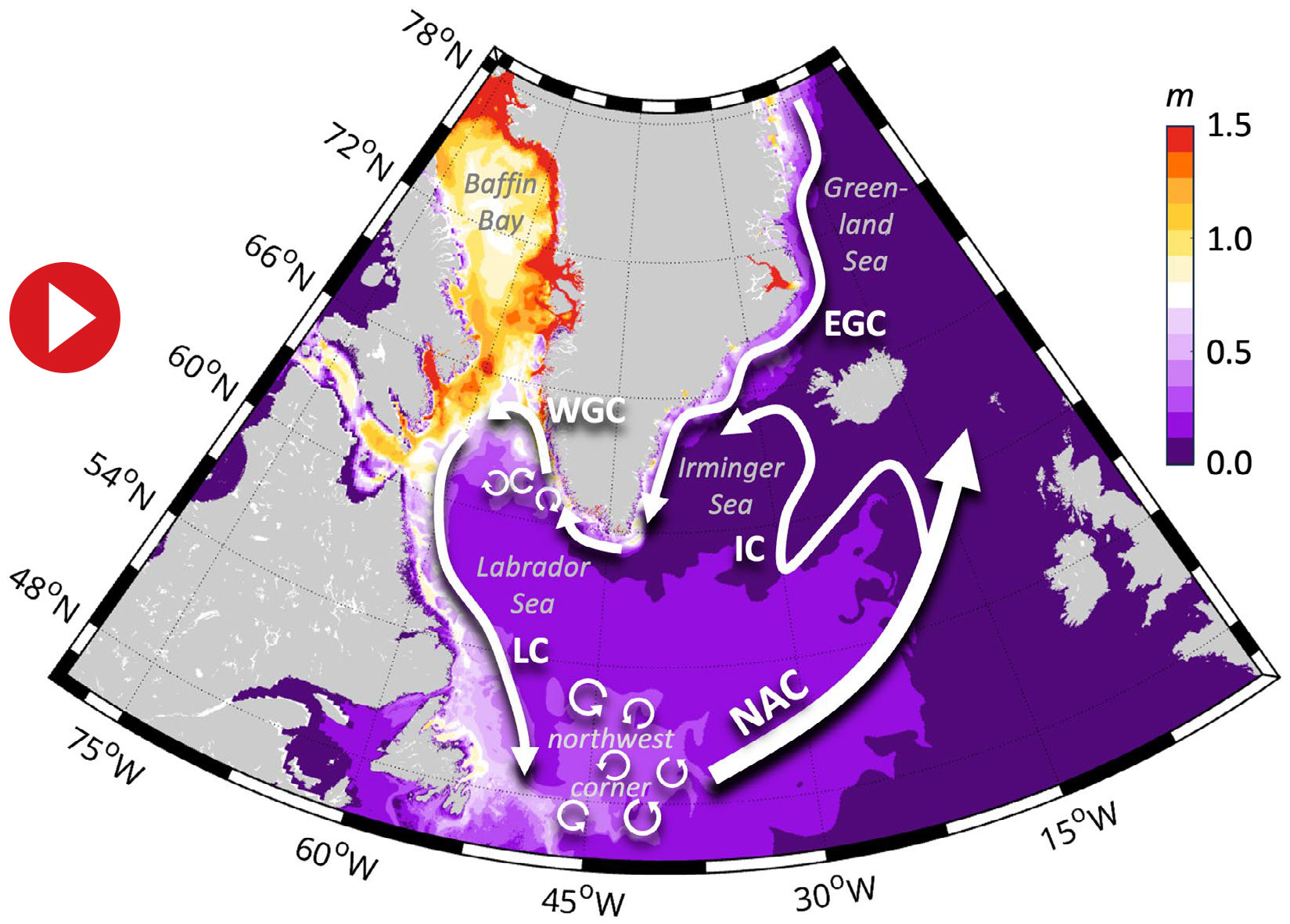
FIGURE 6. Annotated snapshot of an animation of the depth integrated concentration of a Greenland discharge passive tracer (with the amount of tracer added in any grid point and timestep proportional to the amount of liquid discharge input into the model from Greenland, based on Bamber et al. [2018]). See Pennelly and Myers (2020) for further details on the model configurations, experiments and tracer setup. Bold arrows indicate the major ocean currents. Circular arrows depict key sites of prominent eddy mixing. NAC = North Atlantic Current. IC = Irminger Current. EGC = East Greenland Current. WGC = West Greenland Current. LC = Labrador Current. > High res figure
|
With most Greenland-origin freshwater being transported in the West Greenland Coastal Current and West Greenland Current (see earlier section on Fjord-Shelf and Shelf Break), it typically only enters deep convection sites in the Labrador Sea after leaving the shelf on the very western flank of the Labrador Sea (Gillard et al., 2016) and recirculating with the subpolar gyre. The region called “northwest corner” (Lazier, 1994) off Newfoundland acts as a key transition zone for freshwater export. Here, wind forcing (Holliday et al., 2020) and strong mesoscale eddy activity (Zhai et al., 2004) regulate the mixing and offshore export of relatively fresh Polar Water, including Greenland meltwater, that is carried southwestward by the Labrador Current and then entrained into the northeastward-flowing North Atlantic Current (NAC; Jutras et al., 2023). Model simulations show strong sensitivity to resolution here: coarse models tend to overestimate direct eastward export to the NAC, while eddy-rich models indicate gradual entrainment along the NAC pathway (Böning et al., 2016; Martin and Biastoch, 2023). This pathway influences not only surface export but also the formation of Labrador Sea Water at depth, where Greenland freshwater can be incorporated during deep convection in the central Labrador Sea (Yeager et al., 2021).
The northwest corner is also an important transition zone between the subtropical and subpolar gyres (Buckley and Marshall, 2016), where the coherence of the AMOC is thought to weaken or break down (e.g., R. Zhang, 2010). In this region, it is uncertain whether subtropical waters continue northward and subpolar waters continue southward, but any exchange between these flows likely controls whether anomalies in one gyre are transmitted to the other (Buckley and Marshall, 2016). A leading hypothesis is that this exchange would be driven by the zonal density gradient across the region, with denser waters in the west and lighter waters in the east (Yeager et al., 2021; Chafik et al., 2023; Madan et al., 2024). Because Greenland freshwater is mainly added along the western boundary, it may weaken this density contrast by freshening (and thus lightening) the western side. This would reduce the cross-gyre density gradient and could weaken the AMOC. In this sense, Greenland meltwater may influence the AMOC not only through deep convection regions but also by modifying the large-scale density structure that helps control inter-gyre exchange. However, this mechanism remains speculative and requires further investigation.
Once within the NAC, Greenland freshwater is dispersed across the eastern North Atlantic. In winter, strong surface heat loss in this region drives the transformation of warm, salty Atlantic Water into dense North Atlantic Deep Water, a key component of the overturning circulation (Lozier et al., 2019). It has been hypothesized that sufficiently large Greenland freshwater input could eventually freshen the surface, shoal the mixed layer, and enhance stratification, thereby reducing winter heat loss. However, the present-day Greenland runoff (~0.01 Sv) is about two orders of magnitude smaller than typical local precipitation (~4 mm d–1; Behrangi et al., 2024), which is also expected to increase with warmer air temperatures and an accelerated hydrological cycle in the future. In addition, air-sea heat fluxes are expected to adjust to a weaker AMOC state through atmospheric feedback (i.e., a cooler ocean surface creates a cooler overlying atmosphere) so that the ocean-atmosphere temperature difference remains largely unchanged and the net heat exchange is only weakly affected (Martin and Biastoch, 2023). Freshwater or salinity variability in the eastern North Atlantic is also tightly linked to upstream dynamics in the northwest corner and the Labrador Sea, with atmospheric circulation acting as a key control on freshwater export from the shelf (Holliday et al., 2020; Fox et al., 2022).
From the eastern North Atlantic, Greenland freshwater either recirculates in the subpolar gyre and enters the Irminger Current (Devana et al., 2021), or it enters the Nordic Seas with the Norwegian Current. In the Nordic Seas, Atlantic water density is increased by heat loss and, to a smaller extent, by brine rejection during sea ice formation. The resulting deep water exits through overflows along the Greenland-Scotland Ridge into the subpolar North Atlantic, forming the dominant branch of the AMOC at these latitudes (Lozier et al., 2019). Freshwater in the Irminger Current circulates around the Irminger Sea and is typically found farther offshore along the continental slope, compared to freshwater that is directly discharged from the East Greenland coast and remains confined to the coastal boundary current system (see section on Fjord-Shelf and Shelf Break). In this more offshore position, freshwater can be more readily transported toward deep convection regions through eddy exchange, albeit in a more diluted form. Hence, in the Labrador Sea, it is primarily eddies shed from the Irminger Current that deliver freshwater into the deep convection region (Rieck et al., 2019; Pennelly and Myers, 2022). Recent increases in Greenland freshwater flux have been linked to an acceleration of the boundary current system and a slight upstream shift in the eddy-shedding region of the West Greenland Current (Schiller-Weiss et al., 2024).
In summary, the long-standing assumption that deep convection in the subpolar North Atlantic directly controls the strength of the overturning circulation has come under increasing scrutiny (Lozier, 2012; Frajka-Williams et al., 2016). If deep convection in the Labrador Sea constituted the primary source of dense waters feeding the overturning circulation, the rate of dense-water formation should match the overturning transport itself. However, a persistent mismatch found in recent observations from the OSNAP array between convective intensity and overturning strength indicates that this linkage is far weaker than previously assumed (Lozier et al., 2019). Labrador Sea convection rather acts on water masses that are repeatedly transformed and recirculated before contributing to the AMOC (Böning et al., 2023), reflecting a sequence of processes that modify the formation rates and properties of different modes of North Atlantic Deep Water, which together feed the lower limb of the AMOC (Zou et al., 2020; Tooth et al., 2025). These processes operate across a wide range of magnitudes and timescales (Johnson et al., 2019), from rapid distribution within eddies shedding from the boundary currents (weeks to months; van Westen et al., 2025) to basin-scale gyre adjustment (years to decades), and they are sensitive to freshwater inputs that are in many cases larger than the observed recent increase in Greenland mass loss (see section on How Much Freshwater is Released From the GrIS?). This multiscale response is further modulated by atmospheric variability, including wind regime shifts (Holliday et al., 2020), air–sea heat flux changes over the Labrador Sea (Fox et al., 2022; Böning et al., 2023), and wind-driven cross-shelf transport variations (Castelao et al., 2019). As a result, the response of the system to Greenland freshwater forcing is not immediate but mediated by multi-year pathways, which can explain the (multi-)decadal adjustment timescales seen in models following stepwise freshwater perturbations (e.g., L.C. Jackson and Wood, 2018; Martin and Biastoch, 2023). In addition, decadal variability observed in the formation and export of lower North Atlantic Deep Water at the 53°N western boundary has been linked to shifts in the North Atlantic Oscillation, further underscoring that overturning variability arises from a combination of basin-wide dynamical processes rather than from Labrador Sea convection alone (Zantopp et al., 2017). As a consequence, suppressing convection through freshwater inputs from Greenland or the Arctic is unlikely to reduce the overturning directly, at least not via the classical mechanism of “shutting down” Labrador Sea convection.
Representing this coupled sequence of processes in numerical models remains challenging. Surface heat loss depends on the ocean-atmosphere temperature gradient and the relative positioning of the North Atlantic Current and atmospheric westerlies, making it sensitive to horizontal resolution (Grist et al., 2018; Kostov et al., 2019; Martin and Biastoch, 2023). Indeed, surface heat flux anomalies have recently been used as a proxy for AMOC variability in climate models (Li and Liu, 2025; Terhaar et al., 2025), complementing earlier approaches using sea surface temperature fingerprints (Rahmstorf et al., 2015; Caesar et al., 2018). Vertical resolution and coordinate choice (depth vs. density coordinates) are critical for representing overflows between the Nordic Seas and the North Atlantic; insufficient resolution can lead to excessive numerical mixing and diffusion of dense waters. While newer model configurations have improved this representation, they come with increased structural complexity (Legg et al., 2009; Colombo et al., 2020; Bruciaferri et al., 2024). Despite these improvements, large-scale simulations still exhibit biases in both the intensity and the location of deep convection in the Labrador Sea and Irminger Sea (Heuzé, 2021; Koenigk et al., 2021), leading to an overemphasis on Labrador Sea convection as a control on AMOC variability (Heuzé, 2021; Yeager et al., 2021). This represents a major uncertainty in projections of the AMOC response to future Greenland meltwater input.
Summary and Conclusions
This review examines what is known and what remains unknown about the fate of Greenland’s freshwater, from its release at the ice sheet to its potential influence on the AMOC. Overall, existing research provides a robust qualitative understanding of the individual components of the Greenland freshwater system. Freshwater is substantially modified at the fjord scale through plume-driven mixing, circulation constrained by sills, and interactions with fjord stratification, before encountering shelf currents. These currents then limit cross-shelf exchange, with winds and mesoscale eddies introducing strong spatial and temporal variability, and subsequent water mass transformation during (re-)circulation in the North Atlantic. We also know that the manner in which freshwater from the GrIS enters the ocean matters because of its ultimate influence on ocean circulation, deep convection, and overturning. Many modeling studies have relied on highly idealized freshwater hosing experiments in which meltwater is distributed uniformly over large regions of the North Atlantic. While useful for exploring first-order sensitivities, these approaches neglect key processes that we know are shaping Greenland freshwater pathways in the real ocean.
The greatest unknowns lie not in identifying the relevant processes, but in quantifying their relative importance and their cumulative influence across scales. We still know relatively little about the spatial and temporal variability within individual subsystems, the interactions between competing processes, and how faithfully these processes are represented in numerical models. A more realistic representation of where, when, and how Greenland freshwater enters the ocean could substantially alter simulated circulation patterns. At present, there is an unavoidable mismatch between the scales at which key freshwater processes occur and the models used to study the AMOC: Earth system models and global ocean general circulation models simply cannot be run at the resolution required to faithfully capture Greenland freshwater pathways. Consequently, the sensitivity of the AMOC to a given freshwater perturbation remains poorly constrained, and significant uncertainty persists in projections of how continued Greenland Ice Sheet melt will influence the climate system.
Addressing these uncertainties requires that observations and models be developed together. A major observational challenge is that Greenland freshwater must be tracked from its sources, across the continental shelf, and into the basin interior over interannual to decadal timescales. Although targeted field campaigns have considerably advanced our understanding of fjord and shelf processes, observations will remain too sparse to constrain freshwater pathways throughout the subpolar North Atlantic, as the large spatial extent, three-dimensional structure, and relatively weak freshwater signal make it unrealistic to resolve these pathways through observations alone. Future observing systems should therefore be designed not only to document freshwater transport, but also to constrain and improve the parameterizations needed to represent unresolved processes in climate models, including fjord-scale transformation, surface-layer dynamics, and eddy-driven transport.
Finally, Greenland meltwater is only one of several freshwater sources influencing the North Atlantic. Other factors beyond direct Greenland freshwater input might play an even larger role in future AMOC changes, including altered wind patterns, heat fluxes, and sea ice processes. In particular, global warming itself may exert a stronger influence on the overturning circulation than the freshwater forcing component (Gregory et al., 2024). Modeling studies of AMOC responses to Greenland freshwater input remain powerful tools for exploring mechanisms and potential outcomes, but their results must be interpreted in the context of their assumptions and limitations. An honest assessment of uncertainties is essential if these studies are to inform our understanding of regional and global consequences of continued Greenland ice loss.
Acknowledgments
The idea for this study was formed in a working group organized by the NSF-AccelNet-2020387 GRISO project (ATN, KS). KS, ATN, and SM received funding through US National Science Foundation grant NSF-OPP 2335928. KS and ATN received support from National Science Foundation grant NSF-OCE-2401413. EFW was funded through the Horizon Europe EPOC project (101059547) and TERIFIC project (803140). Views and opinions expressed are those of the author(s) only and do not necessarily reflect those of the European Union. Neither the European Union nor the granting authority can be held responsible for them. NPF was supported by grants NSF-OCE-2421096 and NSF-OCE-2123128. JLB was supported by the Technical University of Munich – Institute for Advanced Study, Germany and European Union’s Horizon 2020 research and innovation programme through the project Arctic PASSION (grant number: 101003472). PGM received funding through a Natural Sciences and Engineering Research Council of Canada (NSERC) Grant RGPIN-2020-04344, as well as computational support from an allocation provided by the Digital Research Alliance of Canada. RHJ received funding support from National Science Foundation grant NSF-OCE-2023415. We thank three anonymous reviewers for their input, which improved this manuscript.
Data Availability Statement
The Fortran code used to conduct the LAB60 simulations was based on the NEMO model and can be accessed from the NEMO version 3.6 repository (https://www.nemo-ocean.eu/ and https://forge.ipsl.jussieu.fr/nemo/ browser/NEMO/releases/release-3.6). Details on the LAB60 experiments can be found in Hoshyar et al. (2024) and Pennelly and Myers (2020), and the files for the reference experiments are available in Pennelly (2020). The initial and boundary conditions, atmospheric forcing, and numerical output were too large to host on a repository and are instead hosted on internal servers as well as the Digital Research Alliance of Canada Trillium server.


 PDF