Effective management of deep-sea ecosystems and the high seas is hindered by the absence of a globally consistent framework for characterizing benthic habitats. Here we present the first global ecological classification of the seafloor, comprising 250 unique ecological benthic units (EBUs), distributed on the seafloor as nearly 700,000 EBU polygon occurrences, generated by intersecting a high-resolution geomorphic map with multivariate environmental seascapes. Using 17 million seafloor data points and 0.05° resolution biophysical datasets—including bottom temperature, dissolved oxygen, pH, carbon flux, sediment thickness, crustal age, and bottom currents—we identified 57 benthic regions across six major geomorphic groups (shelves, slopes, seamounts/guyots, spreading ridges, abyssal/hadal areas, plateaus). The resulting EBUs reveal previously unrecognized ecological gradients, quantify global patterns of benthic heterogeneity, and expose large-scale environmental vulnerabilities. Notably, we find that 95.6 million km² (26% of the ocean area) of abyssal seafloor lies below the carbonate compensation depth, that 4.16 million km² (1% of the ocean) of continental slopes intersect severe oxygen minima, and <1% of seamounts occur in seascapes most environmentally favorable to life. These insights provide a powerful basis for identifying rare habitat configurations, assessing exposure to climate-driven stressors, and prioritizing areas for high seas marine protected area planning, as well as a policy-relevant foundation for environmental impact assessment and biodiversity baseline proxies under the new United Nations High Seas Treaty.

Introduction

Society’s interest in exploiting deep-sea resources is growing rapidly, but the same cannot be said for our ability to effectively conserve and manage the deep ocean (>500 m depth) and high seas (i.e., international waters beyond national jurisdiction). The recent ratification of the United Nations (UN) High Seas Treaty (formally the Agreement on Marine Biological Diversity of Areas Beyond National Jurisdiction or BBNJ Agreement; High Seas Alliance, 2025) indicates that there is a growing need to conserve the ocean’s resources and protect the biodiversity that it contains. There have been discussions of what aspects should be considered when planning conservation strategies for the deep ocean realms (Ceccarelli et al., 2021), but there remains a lack of sufficient tools and data to guide decision-making processes (McQuaid et al., 2023; Misiuk and Brown, 2024).

1. Marine spatial planning in the ocean, including the high seas areas, involves making decisions about managing human activities in the ocean. For example:
2. Sustainable harvesting of living marine resources and conservation of biodiversity: There is growing interest in harvesting deep-sea biological resources for food and the genetic materials used in the development of pharmaceuticals (Bisson et al., 2023).
3. Understanding impacts of pollution: For example, deep-sea sediments are the final resting place for plastic pollution lost in the ocean. However, our understanding of pathways and what environments are most impacted is very poor (Harris et al., 2023). This includes creating more accurate environmental impact assessments for potential deep-sea resource extraction.
4. Establishment and monitoring of high seas marine protected areas: To create an ecologically representative global network of marine protected areas (MPAs) as per the new UN Highs Seas Treaty, we first need to understand the spatial distribution of different seabed environments and the biodiversity they contain. Our understanding of deep-sea habitats is still extremely limited, illustrated by the recent extraordinary discovery of the electrochemical production of “dark oxygen” on the abyssal seafloor by polymetallic nodules (Sweetman et al., 2024).
5. Understanding impacts of climate change: Research shows that global climate change is driving changes in deep ocean pH (Sulpis et al., 2018), bottom currents, and patterns of sedimentation. Further, the shape of the seafloor combines with these factors to influence the amount of heat flowing underneath ice shelves and contributing to melting (Richter et al., 2025). Deep-sea biota will respond to these ecosystem changes by moving and/or recolonizing different locations that suit their needs (Ramirez-Llodra et al., 2011).

In this paper, we present a new benthic classification that we call “ecological benthic units” (EBUs) for the world ocean. Our aim is to provide a new tool to improve global understanding and decision-making capability for a range of global issues, as listed above. EBUs build upon an earlier map of ecological marine units (EMUs) that characterizes the ocean water column as a proxy for pelagic ecosystems (Sayre et al., 2017). As abiotic surrogates for benthic biodiversity (McArthur et al., 2010; Astudillo-Scalia et al., 2021), the EBUs are environmentally distinct areas occurring within physiographically stratified geomorphic types, and they represent the ecological settings that control the distribution of benthic biota.

 

Approach Taken

The global map of seafloor geomorphic features (Harris et al., 2014) provides the basis for the present study. It contains 29 seafloor feature categories, such as submarine canyons, seamounts, mid-ocean ridges, troughs, rift valleys, escarpments, and basins. The map divides the global ocean floor into more than 120,000 separate polygons and provides the basis for quantitative classification of seafloor areas. Seafloor geomorphology, mapped and measured by marine scientists, has proven to be a very useful physical attribute for ocean management. This is because different geomorphic features (e.g., submarine canyons, seamounts, spreading ridges, escarpments, plateaus, trenches) are commonly associated with particular suites of habitats and biological communities (Harris and Baker, 2020). The features themselves, be they canyons, sea valleys, rocky reefs, or sand banks, become the shorthand descriptor (if not the direct focus) of conservation efforts and marine management processes because they are easily understood by the broader community and are commonly associated with a particular kind of benthic community.

To advance the science underpinning ocean conservation, better classification resolution and spatial resolution are needed to sub-classify geomorphic features into more meaningful EBUs. We used existing spatial datasets for environmental parameters relevant to the deep-sea ecosystem. For example, six ecologically relevant biophysical variables (depth, seabed slope, sediment thickness, primary production, bottom water dissolved oxygen, and bottom temperature) were used by Harris and Whiteway (2009) to classify the ocean into 53,713 separate polygons comprising 11 different categories called ‘‘seascapes.’’ A similar approach was used by Sayre et al. (2017) to create the EMU ocean water column classification. In this paper, we subclassify the existing map of seafloor geomorphic features into different sub-units with existing spatial data using multivariate statistics.

 

Ecological Significance of Variables Used and Derived

Reviews of the ecological significance of biophysical variables used for global seascape type analyses such as those conducted for the present study have been published previously (e.g., Harris and Whiteway, 2009). The input variables used may be grouped into four broad categories: (1) physical/structural (depth​, seafloor gradient​ [slope)], feature height​ above seafloor, crustal age, spreading rate​, sediment thickness); (2) chemical (water temperature, pH, dissolved oxygen, salinity); (3) biological (primary productivity, seafloor downward organic carbon flux); and (4) hydrodynamic (sea ice cover, significant wave height, tidal range, benthic current velocity).

The use of static variables (e.g., annual mean value when seasonal variations are present) to characterize the ocean has clear limitations. The occurrence of biota at any given location on the seafloor will not necessarily be in response to the mean value of any variable. Dynamic aspects of the benthic environment include natural changes in variables like current speed, temperature, dissolved oxygen, and food supply. It is now an established fact that there are “benthic storms” (e.g., Woodgate and Fahrbach, 1999) and seasons in the deep sea. Detrital-feeding fauna and suspension-​feeding organisms have evolved to exploit the seasonal, vertical flux of surface matter sinking to the seabed. Seasons are recorded by moored sediment traps (e.g., Juniper et al., 2013) and in thick versus thin growth rings in the shells of small abyssal molluscs (Gage and Tyler, 1991). A key driver for longer-frequency (>1 year) variations is change in deep ocean (near bottom) current speed and/or direction. Because water properties are essentially carried passively over benthic habitats in the moving water column, changes in bottom currents can trigger changes in (for example) the quantity and quality of particulate organic carbon (POC) flux (food) to the abyssal seafloor (Smith et al., 2008). For this reason, we include modeled bottom water current speed and direction in our analysis.

Examples of derived variables include local benthic habitat heterogeneity (e.g., number of unique EBU types per neighborhood) and orientation of seafloor features to the prevailing current. Several authors have reported evidence that seafloor heterogeneity is an indicator of areas with high species richness (e.g., Harris, 2012; Zeppilli et al., 2016; Riehl et al., 2020; Zhao et al., 2020; Romoth et al., 2023). In this study, we quantify the number of polygons per unit area to compare the heterogeneity of seascapes and their associated geomorphic features.

Some seafloor features rise up prominently, providing a hard, rocky substrate that is habitat for sessile benthic animals that rely upon filter-feeding plankton and organic detritus from the water column for their food supply. The optimum orientation of such a substrate is one that faces into the prevailing current, thus bringing the most amount of suspended detritus (food) to the waiting tentacles (Baynes and Szmant, 1989). In this study we include an analysis of seafloor feature orientation relative to the modeled bottom current.

 

Methods

Creating Seafloor Geomorphology as a Single Map Layer

The project builds upon the foundation of an existing 1 km global grid of seafloor geomorphic features (Harris et al., 2014) that was based on bathymetric data available at the time, in particular, the SRTM 30_PLUS model of Becker et al. (2009). Although the global bathymetry database is improving every year, it is beyond the scope of this project to produce a revised/updated version of the 2014 global seafloor geomorphic features map.

The geomorphic features were first “flattened” in ArcGIS Pro 3.6 to remove all areas of spatial overlap. This flattening was performed through a hierarchical overlay process in which the 28 geomorphic feature types were prioritized based on their logical order of superposition. Superimposed features were sequentially “burned into” those below them in the hierarchy. For example, a canyon cutting across a slope that ends on an abyssal plain would overwrite the slope and abyssal plain where it intersects them, while the slope and abyssal plain would remain elsewhere. This resulted in a single map layer where every grid point was allocated into a single geomorphic feature type. Table 1 lists the 28 feature categories used in this study. We did not include escarpments mapped by Harris et al. (2014) because these were measured from bathymetry (gradient exceeding 20°) and draped over other features (e.g., ridges with escarpment, canyons with escarpment). Hence “escarpment” is a secondary attribute of other features.

 

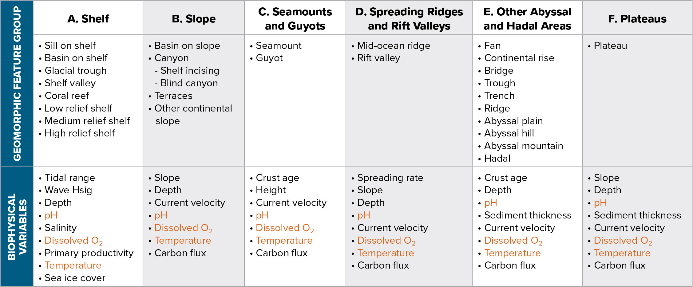
TABLE 1. List of the geomorphic feature groups (A–F) and their associated biophysical variables used for sub-classification in this study. Seascapes were derived separately to match six different groups of seabed geomorphic features: (A) shelf, (B) slope, (C) seamounts and guyots, (D) spreading ridges and rift valleys, (E) other abyssal and hadal areas, and (F) plateaus. Variables common to all groups are shown in orange text. > High res table

 

Establishing Geomorphic Groups

The next step was to allocate relevant biophysical variables to each of the geomorphic features. Geomorphic feature types were grouped into six broad geomorphic groups—continental shelf, continental slope, seamounts and guyots, crust-forming, complex/deep seafloor, and plateaus—to reflect fundamental differences in ecological drivers and physical processes across the seafloor. This grouping allowed for a more targeted selection of environmental variables within each geomorphic group. Although a number of data layers covering the global ocean (or specific areas of the global ocean) are available, not every data layer is necessarily relevant to sub-classifying a given geomorphic feature. For example, ocean surface waves may impact the shallow continental shelf but have no impact on mid-ocean spreading ridges. Conversely, seafloor spreading rate is an important characteristic of mid-ocean rift valleys but is not relevant to shallow coral reefs. Therefore, relevant biophysical variables were allocated differently for each geomorphic group (Table 1). In short, we clipped the biophysical data to geomorphic group geographies, performed a cluster analysis within each geomorphic group, subdivided the geomorphic group into seascapes using the clustered biophysical data, and then summarized distribution of those seascapes among geomorphic feature types, as follows.

 

Seascapes

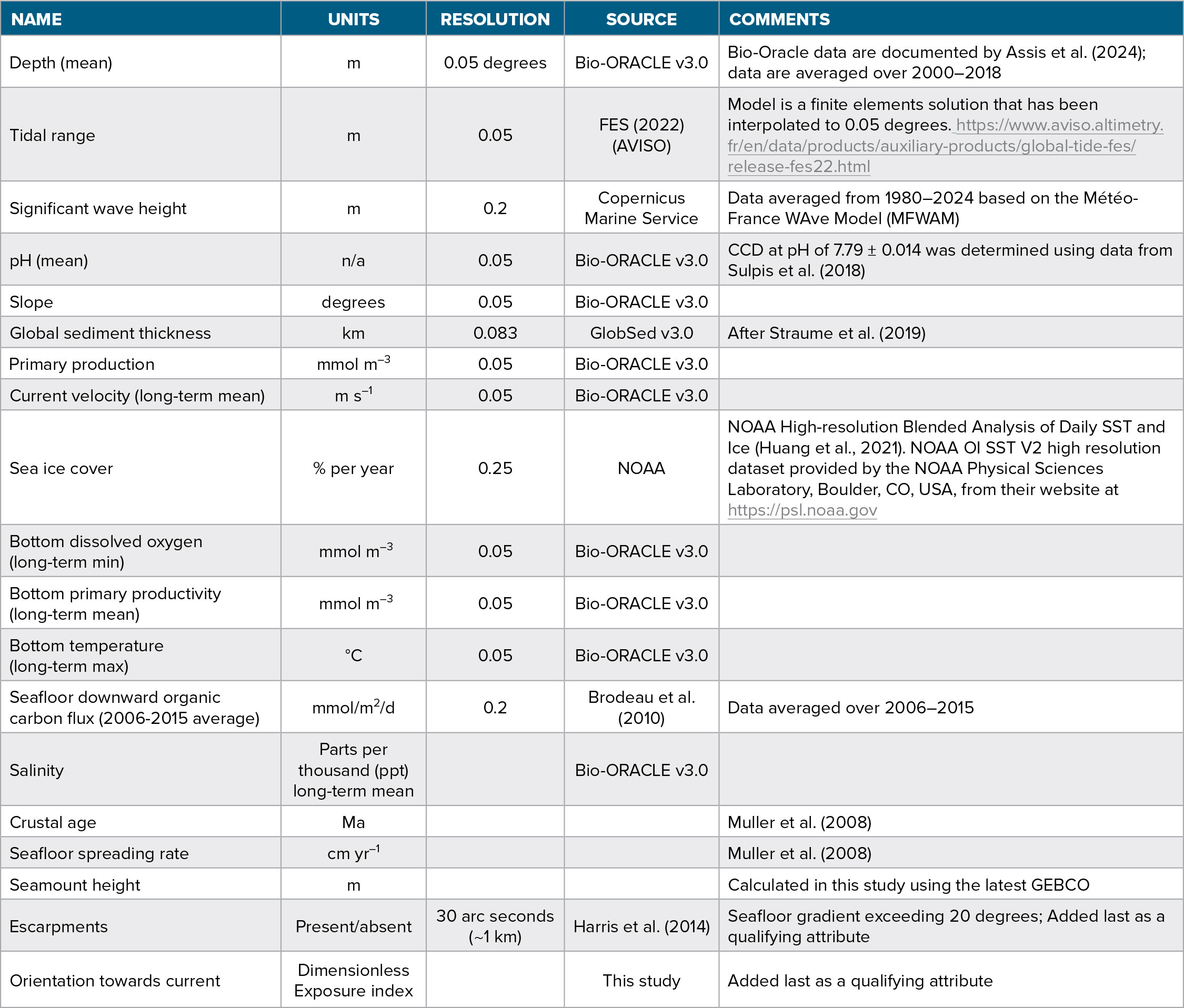
Within each of the six geomorphic groups (Groups A–F), a separate K-means clustering analysis was carried out based on the biophysical variables as they are aligned in Table 1. The main data source was Bio-Oracle (Assis et al., 2024), a gridded product at a pixel spacing of 0.05° (~6 km); all data sources are listed in Table 2. To prevent variables with a higher variance from having more influence in the clustering, we standardized each variable to a mean of zero and a standard deviation of one before clustering. We then created a regular global grid of points covering the seafloor at 0.05° resolution (approximately 5.5 km at the equator), yielding 17,034,951 points. This resolution was chosen to match the Bio-ORACLE v3.0 dataset, which provided most of the physiochemical variables used in the analysis. Each point of the global mesh was assigned to one of the six geomorphic groups based on its location within the flattened geomorphic layer. Environmental variables were extracted from a series of raster datasets (Table 2), some with differing cell sizes and spatial alignments.

 

TABLE 2. List of variables used in this study, with units, data source, and resolution. The variables “Escarpments” and “Orientation towards current” were not used as inputs to the K‑means clustering. They are derived attributes added after clustering to provide additional environmental context for the resulting EBUs and to support future analyses by other researchers. They do not influence cluster assignments or polygon boundaries in this study. > High res table

 

To ensure consistent attribution, values in Table 2 were assigned to points using nearest neighbor resampling, which assigns the value of the raster cell containing the point without interpolation. Importantly, the specific geomorphic feature type (e.g., “sill on shelf” or “guyot”) was not included as an input variable, allowing the clustering to remain blind to the geomorphic feature type. For pixels with slope >3°, current direction was assessed relative to pixel aspect. Currents flowing from 90° to 270° relative to aspect were classified as high relief exposed, whereas currents flowing from 270° through 0° to 90° were classified as high relief sheltered.

For each geomorphic group, we constructed a cross-correlation matrix to assess redundancy among variables. Variables with correlations greater than 0.7 were removed to reduce redundancy and ensure that no single type of environmental condition was overrepresented in the analysis. This helped ensure that each variable contributed more equally to the clustering process.

Clustering was conducted separately for each geomorphic group using K-means clustering in SAS. The number of clusters tested ranged from 3 to 25. The optimal number of clusters for each group was selected using the “gap statistic” (Tibshirani et al., 2001), which compares the within-cluster dispersion to that expected under a null reference distribution. The optimal number corresponds to the highest significant peak in the gap statistic. Each point was labeled with its final cluster assignment, and these clusters—interpreted as distinct seascape types—were merged across all groups to produce the final global seafloor classification. All variables listed in Table 1 were used in the clustering; no variables were removed post hoc due to cross correlation.

 

Naming of Seascapes and EBUs

Terminology and thresholds describing the environmental variables that establish the class names and value ranges for each class are based on the National Oceanic and Atmospheric Administration (NOAA) Coastal and Marine Ecological Classification Standard (CMECS) scheme, where relevant terms are available (US FGDC, 2012; see online supplementary Table S1). For each of the 57 seascape types identified, the mean value of each environmental variable used in the clustering (Table 1) was calculated, except in the case for temperature and dissolved oxygen, where long-term maximum and minimum values were used to better reflect biologically limiting values (e.g., Baker et al., 2024; Capotondi et al., 2024). Throughout this paper, the term “mean” is used for temperature calculated as the average temperature of the warmest month in the period 2000–2010 and for dissolved oxygen as the average level occurring in the month having the lowest average dissolved oxygen in the period 2000–2010; they are thus mean maximum and minimum values, respectively. All mean values were then assigned descriptive labels using existing thresholds (shown in Table S1), concatenated to form a short descriptive seascape name that summarizes the dominant environmental conditions represented by the cluster. For example, a high‑latitude continental shelf seascape might be labeled as Minimally Tidal, Moderately High Wave Energy, Mesobenthic to Shallow Infralittoral Depth, pH Above CCD, Euhaline, Highly Oxic, Very Low Productivity, Very Cold Temperature, with Moderate Ice.

EBUs inherit the seascape name and append the corresponding geomorphic feature name. As a result, every location on the ocean floor represented in the EBU map is associated with an explicit descriptive label that captures both its environmental setting and its geomorphic context. These labels are provided with the publicly available EBU dataset.

 

EBU Heterogeneity

To identify areas where the greatest EBU heterogeneity occurs, a focal variety analysis of the data was undertaken in ArcGIS Pro 3.6. The focal variety tool determines the number of unique values (or the variety) for each cell location on an input raster within a specified neighborhood and sends it to the corresponding cell location on the output raster. In this study, we used a 100 km search radius (i.e., an area of 31,400 km²) to define the neighborhood, reported here as polygons per 1,000 km². EBU heterogeneity used normalized numbers of EBUs in the neighborhood analysis window, thus taking into account any potential variation in the density of EBU types across the geomorphic groups that may have been caused by differing clustering approaches within the geomorphic groups.

 

Results: Seascapes and Geomorphic Feature Sub-classes

The global map of seascapes (Figure 1) produced in this study divides the ocean floor into 162,687 separate polygons. The following sections describe the 57 seascape types by geomorphic group and assess the intersection of seascapes with the previously mapped geomorphic features.

 

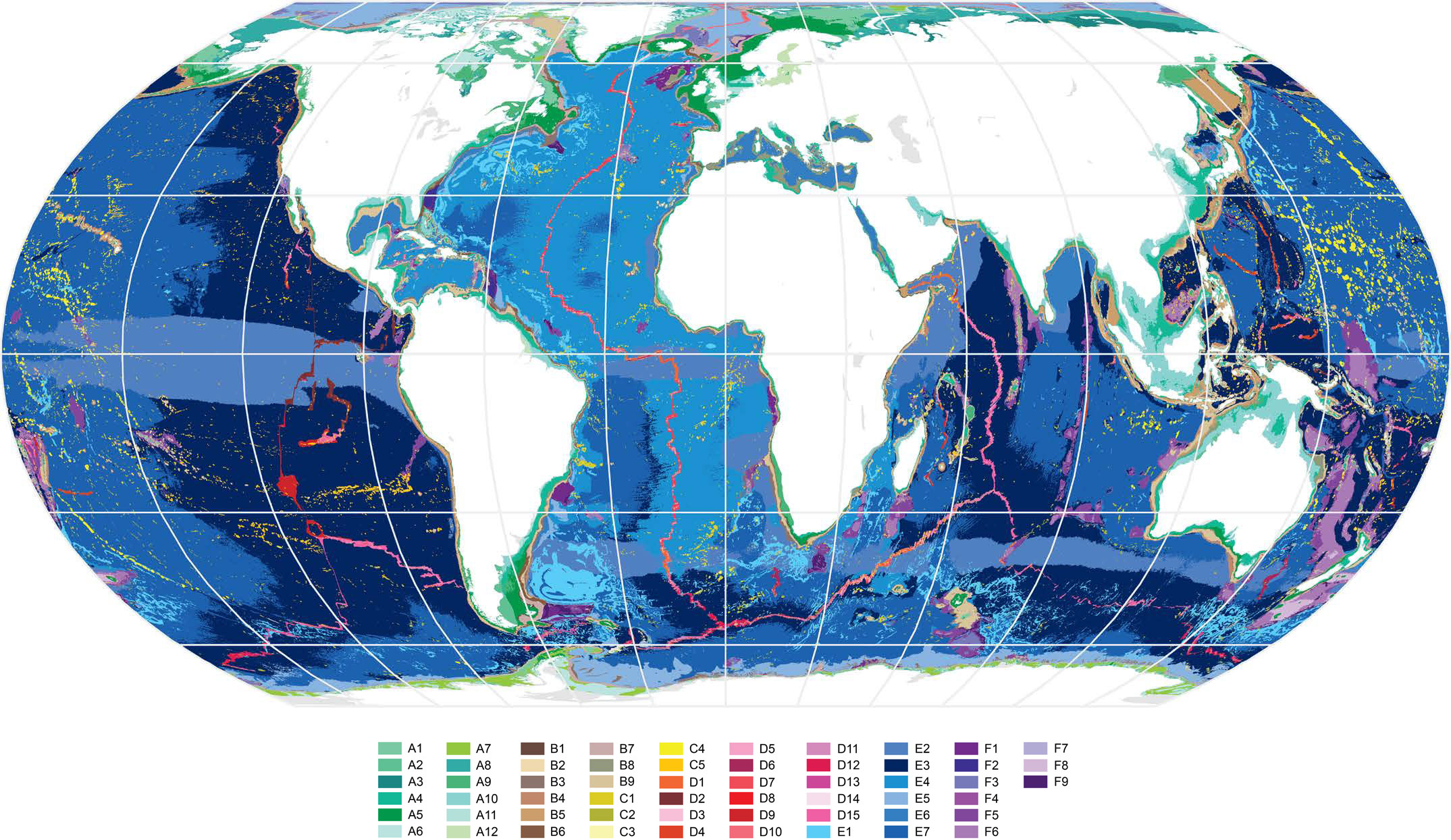
FIGURE 1. Map in Equal Earth projection of the global distribution of 57 seascapes derived for the present project. > High res figure

 

Shelf Seascapes (Group A) and Geomorphic Features

The 12 shelf seascapes fall into three broad categories based on sea ice cover and water temperature: polar, tropical, or temperate. The “polar” category (A1, A3, A6, A7, A8) is characterized by significant sea ice cover (grid cells are ice-covered >70% of the year), cold water (<2.8°C), generally very low to low primary productivity, and the occurrence of geomorphic glacial troughs (Figures 2 and 3). Seascape A1 contains only 0.46 polygons per 1,000 km², making it the least heterogeneous (greater number of large, continuous polygons) of all shelf seascapes.

 

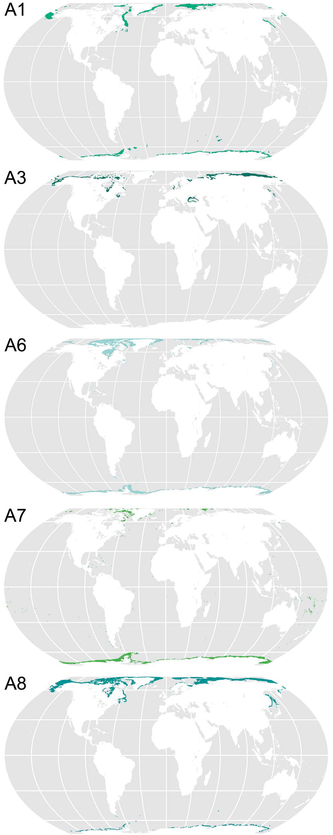
FIGURE 2. Polar shelf seascapes (A1, A3, A6, A7, and A8), mapped in the Equal Earth projection (as per all maps in this paper), derived in the present study. See Table 1 for the list of variables used in the cluster analysis. These seascapes have mean sea ice cover per day of greater than 70% and mean water temperature below 2.8°C. The geomorphic features associated with each seascape are illustrated in Figure 3. > High res figure

 

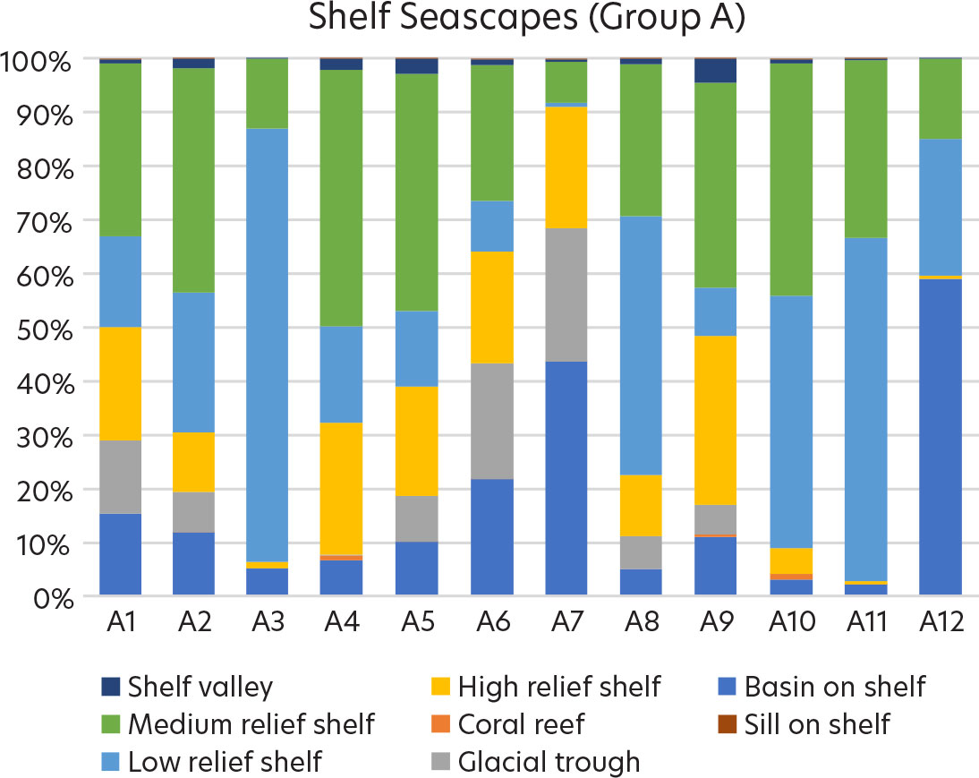
FIGURE 3. Intersection of different shelf geomorphic features with the seascapes, shown as a percent area. The graph shows that each seascape is dominated mainly by different percent areas of low (<10 m), medium (10–50 m), and high (>50 m) vertical relief shelf areas. > High res figure

 

Polar seascape A7 has the deepest mean water depth of all shelf seascapes (602 ± 186 m; 186 m is the standard deviation convention used throughout this paper). This great depth is associated with the greatest occurrence of shelf-perched basins, abundant glacial troughs, and the smallest area of low-relief shelf. A7 also has a low mean temperature (0.24°C), which explains the occurrence of this seascape at some higher latitudes (Figure 2) where the shelf extends deeper and intersects cold water masses.

Seascape A3 stands out with its very shallow mean water depth (15.6 ± 12.5 m), relatively low mean salinity (22 ppt), and very high dissolved oxygen 360 ± 33 mmol m^–³. This seascape is found close to the Arctic coastline and in the Black Sea (Figure 2), and it is the warmest and has the highest primary productivity of the polar seascapes.

There are two “tropical” shelf seascapes (A4 and A10) where mean temperature is over 20°C—this is where 85% of coral reefs occur (Figures 3 and 4). Seascapes A4 and A10 are the largest shelf seascapes by surface area, covering 5,615,274 km² and 6,073,758 km², respectively (Figure 3), totaling 36.7% of the total shelf area (31,894,360 km²). Seascape A10 has greatest area of all shelf seascapes and includes the largest area of coral reefs (57,543 km²), largest area of low-relief shelf (2.8 million km²), 46% of sills, and the second-highest mean tidal range of 2.37 m.

 

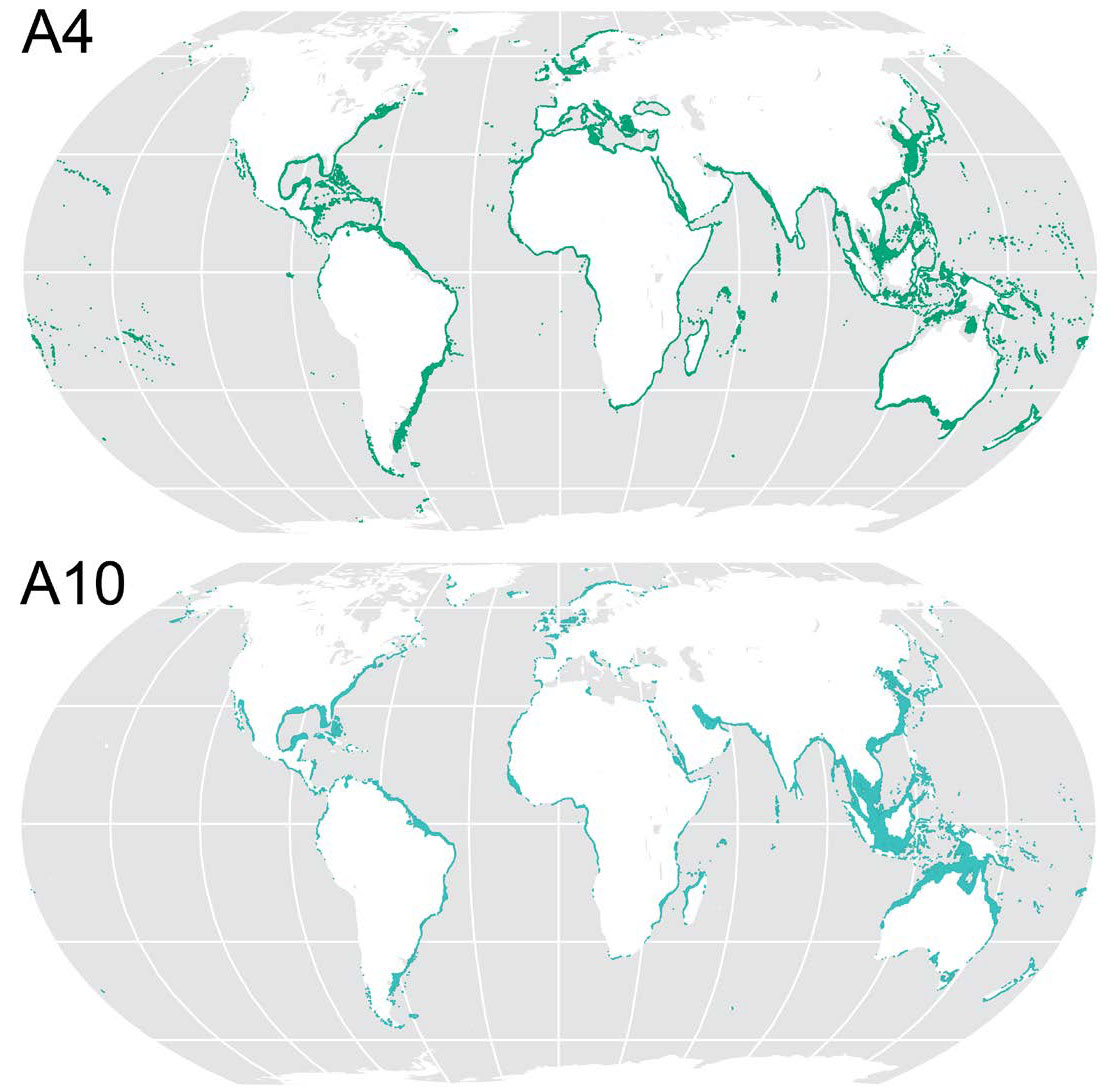
FIGURE 4. “Tropical” shelf seascapes (A4 and A10) derived in the present study are generally located near the equator but do extend to higher latitudes in some places. Seascapes A4 and A10 have mean water temperatures of 20.09o ± 5.75 o C and 29.05° ± 4.71°C, respectively. The geomorphic features associated with each seascape are illustrated in Figure 5. > High res figure

 

Seascape A4 is noteworthy for having the highest mean salinity (34.98 ppt) of all shelf seascapes. It also has the second greatest area of all shelf seascapes and includes the second-largest area of coral reefs (45,081 km²) and the largest area of medium-relief shelf (2.6 million km²), capturing some temperate regions as well (e.g., Stuart-Smith et al., 2017).

The five “temperate” seascapes (A2, A5, A9, A11, and A12) are broadly distributed geographically but have a generally moderate mean temperature range between 3.11°C and 17.97°C. In other respects, these seascapes each exhibit a unique, characteristic attribute. Seascape A2 is the only macrotidal seascape, having a mean, macrotidal range of 5.09 ± 2.06 m, the largest range of all shelf seascapes. This seascape is found on the west European shelf; in the Gulf of Alaska, eastern Canada, and the Sea of Okhotsk; and on the southern Argentine shelf and the Australian northwest shelf.

Seascape A5 exhibits the most energetic wave climate, with a mean significant wave height of 2.94 ± 0.75 m, found around the North Atlantic, Aleutian Islands, southern part of South America, New Zealand, and southern Australia (Figure 5). A5 is also characterized by a significant area of glacial trough.

Seascape A9 is the only hypoxic shelf area with (long-term minimum) dissolved oxygen levels of 94.55 mmol m^–³. It is also characterized by relatively low pH (mean value of 7.7), compared to other shelf waters. This seascape is spatially very strongly associated with western continental margins (Figure 5), which are commonly known as upwelling zones. The upwelled water masses are commonly depleted of oxygen and have a lower pH. Upwelling of deep water depleted in oxygen has been documented in a number of locations associated with boundary currents, including off the coasts of Peru, California (USA), Chile, and West Africa (Chavez and Messié, 2009). The source of the deep water is not necessarily from abyssal depths, but rather mid-depth, oxygen minimum zones. However, there is also evidence that oxygen levels in the global ocean are decreasing in association with anthropogenic climate change and that mid-depth oxygen minimum zones are expanding (Grégoire al., 2021).

 

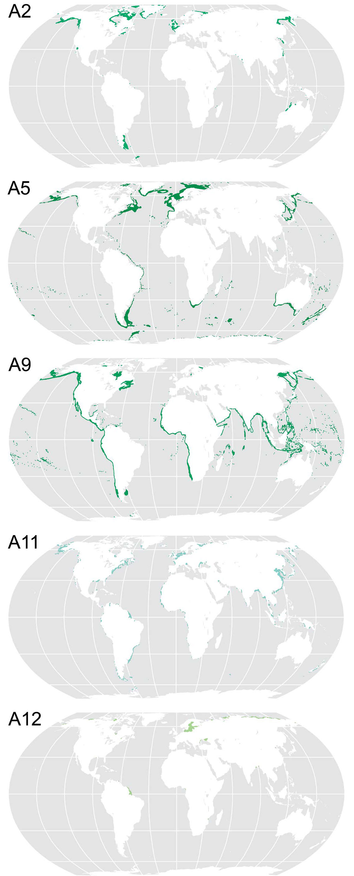
FIGURE 5. “Temperate” shelf seascapes (A2, A5, A9, A11, and A12) derived in the present study generally have mean water temperatures between 3.11°C and 17.97°C. The geomorphic features associated with each seascape are illustrated in Figure 3. > High res figure

 

Seascape A11 is characterized by a very shallow mean depth of 15.86 m, the highest mean pH of 8.07 (most alkaline), and the highest primary productivity, 5.78 mmol m^–³, of all shelf seascapes. A11 is the most heterogeneous of all shelf seascapes, containing 2.57 polygons per 1,000 km². This seascape is broadly dispersed, occurring on the margins of most continents with the exceptions of Australia and the eastern shelf of Africa.

Finally, seascape A12 is classed as “Atidal,” having a mean tidal range of only 0.0693 m; it also has low wave energy with mean significant wave height of 0.91 m, and it has the lowest salinity of all shelf seascapes, only 7.14 ppt. This seascape is geographically constrained to the Baltic Sea, the mouth of the Amazon River, and also adjacent to major Russian and Canadian river mouths that discharge into the Arctic Ocean.

 

Slope Seascapes (Group B) and Geomorphic Features

Slope seascapes are mostly isobath parallel zones of continental margins. Among the most important variables for benthos is the dissolved oxygen regime of the water mass (e.g., Diaz and Rosenberg, 2008; Brietburg et al., 2009; Levin, 2018) impinging on the slope and geomorphic features found along it. Slope seascapes B1 and B5 are characterized by water containing (long-term minima) 72.2 and 52.5 mmol m^–³ dissolved oxygen, making these seascapes hypoxic and severely hypoxic, respectively. Seascape B1 is located at the shallowest mean water depth (285 m) of all slope seascapes, and seascape B5 is the third most shallow seascape (895 m). The pH of bottom water in these two seascapes is also the lowest (most acidic) of all slope seascapes (mean pH of 7.67 and 7.64 for B1 and B5, respectively). Seascape B1 has the highest rate of particulate organic carbon flux (7.12 mmol/m²/d), which is consistent with these areas’ association with ocean upwelling and enhanced primary productivity. Hypoxic seascape geographic distribution is concentrated around the Pacific rim, along the eastern margin of North and South America, in the western Pacific along the coast of Asia, and around Africa, India, New Zealand, and Tasmania (Figure 6). Finally, seascape B1 has the greatest heterogeneity of slope seascapes, 6.7 polygons per 1,000 km², while B5 has the lowest heterogeneity, 0.80 polygons per 1,000 km².

 

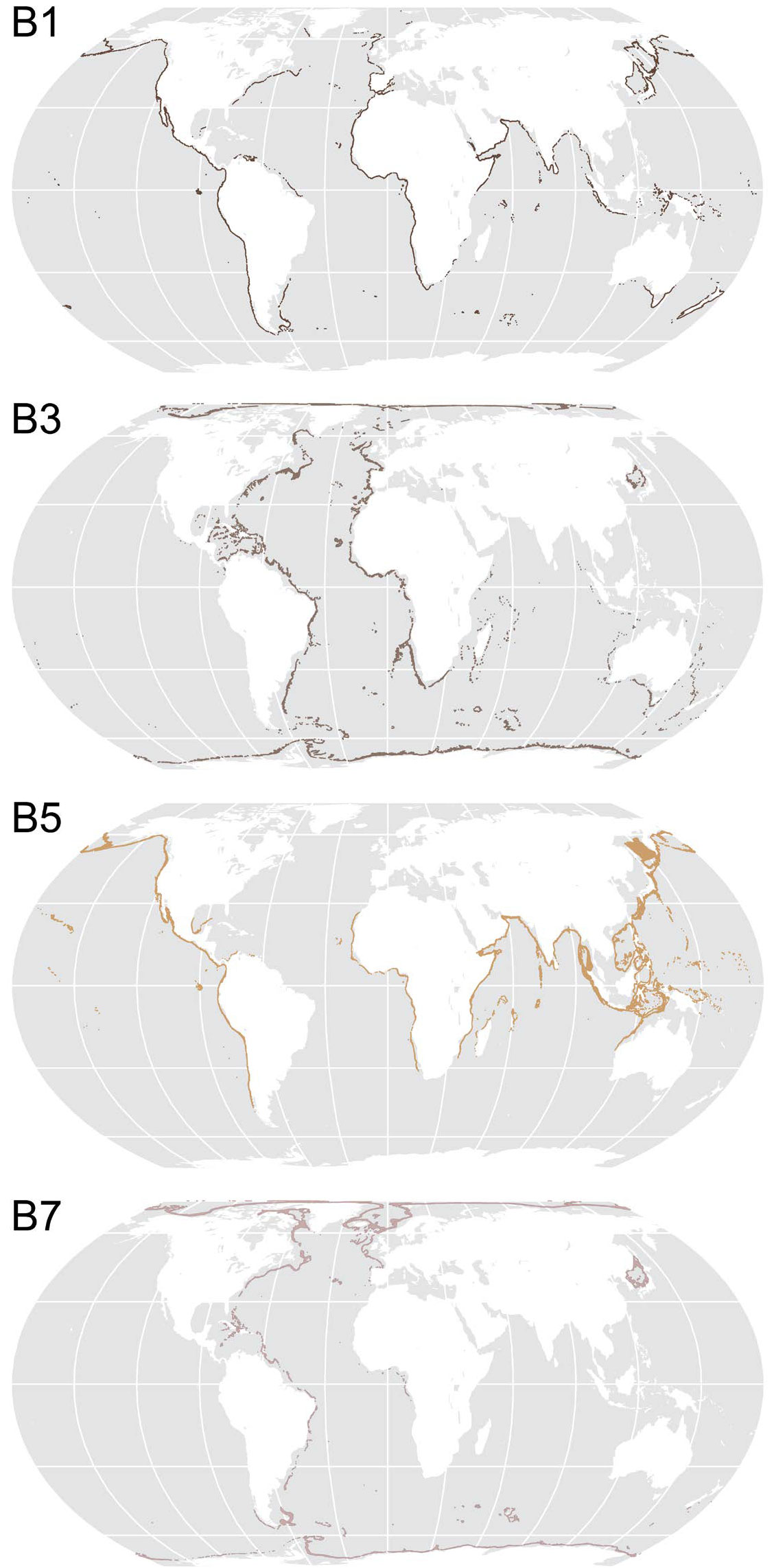
FIGURE 6. Hypoxic slope seascapes B1 and B5 versus highly oxic seascapes B3 and B7. In terms of the depth differences, the mean water depth is 285 m for B1, 895 m for B5, 2,752 m for B3, and 1,112 m for B7. > High res figure

 

In contrast, seascapes B3 and B7 are characterized by the most oxygen-rich waters, containing mean dissolved oxygen levels of 270 and 297 mmol m^–³, respectively. Seascapes B3 and B7 are also characterized by cold bottom water (mean temperatures of –0.07°C and 0.11°C, respectively) and high pH (mean pH values of 7.94 and 8.02, respectively). These well oxygenated seascapes occur at intermediate water depths (2,752 m and 1,112 m, respectively) and are located in both polar seas and along the margins of the Atlantic (Figure 2).

With regard to slope geomorphic features (Figure 7), one obvious association is that about 53.7% of slope-perched basins occur in seascape B9. The depth range of this seascape is 1,581 ± 576 m, and the gradient mean is 1.66°, which characterizes the common locations of slope basins. Submarine canyons occur in all nine seascapes but are most common in polar regions of seascape B3, which contains 32.1% of blind canyons and 22.3% of shelf incising canyons. This is consistent with the observation of Harris et al. (2014) that canyons in polar regions are the largest in the world ocean.

 

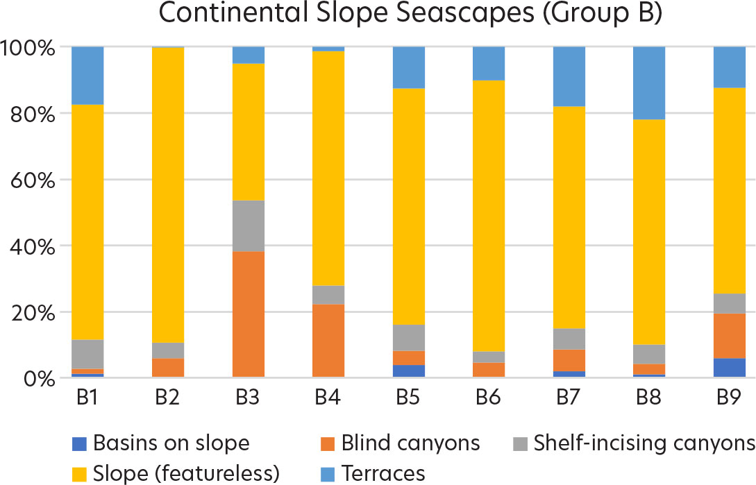
FIGURE 7. Intersection of different slope geomorphic features with the seascapes, shown as a percent area. The graph shows that featureless slope comprises the majority of slope area. > High res figure

 

Seamounts and Guyots (Group C)

The five seascapes created for seamounts and guyots suggest two main categories: Seascapes C1 and C3 (Figure 8) are characterized by warm waters (mean bottom water temperatures of 2.86°C and 8.31°C, respectively) and low to high organic matter flux (mean POC flux of 0.24 and 1.46 mmol/m²/d, respectively). The other three seascapes (C2, C4, and C5) are colder (mean temperature <1.45°C) and exhibit very low POC flux (mean POC flux <0.08 mmol/m²/d).

 

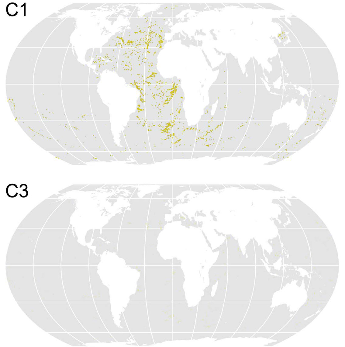
FIGURE 8. Maps show the locations of seascapes C1 and C3, characterized by warm waters and low (C1) to high (C3) organic matter flux. > High res figure

 

Seascape C3 has the greatest heterogeneity of seamount and guyot seascapes with 6.95 polygons per 1,000 km². Compared to deep, cold, low oxygen seascapes (Costello et al., 2023), this seascape appears to provide relatively more favorable conditions for species among seamounts and guyots with warm, oxygenated waters (mean dissolved oxygen is 185 mmol m^–³), good food supply (high POC flux), relatively strong bottom currents (maximum current speed of 0.58 m s^–1), and locations above the carbonate compensation depth (CCD; mean pH is 7.91). However, C3 is also the smallest seamount and guyot seascape at only 81,855 km², representing only 0.94% of the total area of 8,715,301 km² for seamounts and guyots.

Seascape C1 covers more area (1,260,146 km²) but has colder water and low POC flux. Nevertheless, C1 still has oxygenated waters (mean dissolved oxygen is 243 mmol m^–³), relatively strong bottom currents (maximum current speed of 0.4 m s^–1), and is mainly located above the CCD (mean pH is 7.90).

The three cold/low POC flux seascapes (C2, C4, and C5) are generally much larger in area, overall comprising 72.1% of seamount and guyot seascapes. Seascape C4 is the largest among seamount and guyot seascapes at 2.95 million km², and it also has the lowest heterogeneity of 0.72 polygons per 1,000 km².

 

Spreading Ridges and Rift Valleys (Group D)

Multivariate analysis of spreading ridges and rift valleys within slower-spreading ridges identified 15 separate seascapes (Figure 9). Based on mean seafloor spreading rate, the group can be divided into three main categories: slow (<50 mm yr^–1), medium (55–100 mm yr^–1), and fast (>100 mm yr^–1). The “fast” category has only two members, seascapes D2 and D9, which are characterized by having the gentlest mean seafloor gradients (1.13° and 1.23°, respectively) and the lowest mean dissolved oxygen levels (136 mmol m^–³ and 159 mmol m^–³, respectively) of all spreading ridge and rift valley seascapes. Seascape D2 has the lowest heterogeneity among spreading ridge and rift valley seascapes of 0.21 polygons per 1,000 km².

The “medium” category includes four seascapes, D4, D5, D13, and D15, and all nine of the other seascapes are in the “slow” category. The “fast” and “medium” categories are located almost exclusively in the Pacific and Indian Oceans (Figure 9). The seascapes range in size from 20,572 km² (D14) to 1.023 million km² (D15) and have a total area of 6.166 million km². Seascape D3 in the “slow” category has the greatest heterogeneity among spreading ridge and rift valley seascapes of 8.53 polygons per 1,000 km².

 

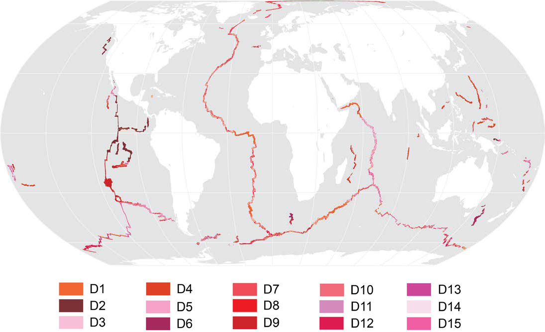
FIGURE 9. Map provides the locations of seascapes D1 to D15, which characterize the mid-ocean spreading ridges and rift valleys. Darker colors indicate faster spreading sub-classes. > High res figure

 

Abyssal Seascapes (Group E) and Geomorphic Features

Multivariate analysis of the abyssal to hadal ocean floor identified seven separate seascapes (Figures 10 and 11). Abyssal seascapes are generally characterized by their very large area (average size of 39.9 million km²) and very low heterogeneity (average of 0.29 polygons per 1,000 km²). Distinguishing and unique aspects that characterize each of the abyssal seascape are as follows:

• E1 – 4.6% of abyssal seascapes by area, has the greatest mean bottom current speed of 0.77 m s^–1.
• E2 – 10.9% of abyssal seascapes by area, has the greatest POC flux of 0.53 mmol/m²/d.
• E3 – 31.9% of abyssal seascapes by area, has the youngest mean age of ocean crust (22.4 million years), the thinnest cover of sediment (mean thickness of 101 m), and the lowest mean dissolved oxygen (176 mmol m^–³). E3 has the largest areas of abyssal mountains, fans, ridges, and troughs (Figure 10). The age of ocean crust is inversely proportional to sediment cover (young crust has had less time for sediment to accumulate; Olson et al., 2016) and hence we expect a relationship between crustal age and the occurrence of rocky substrate versus thick sediment cover habitats.
• E4 – 13.4% of abyssal seascapes by area, has the highest dissolved oxygen of 250 mmol m^–³. E4 has the largest area of continental rise (Figure 10).
• E5 – 3.4% of abyssal seascapes by area, has the coldest mean water temperature of –0.55°C, the lowest mean POC flux of 0.01 mmol/m²/d, and most alkaline waters with a mean pH of 7.93 (equal with E6).
• E6 – 1.5% of abyssal seascapes by area, has the oldest mean ocean crust age at 136.7 Ma, the thickest sediments (mean thickness 6,986 m), most shallow mean depth of 2,679 m, warmest mean water temperature of 3.95°C, and most alkaline waters with a mean pH of 7.93 (equal with E5).
• E7 – 34.3% of abyssal seascapes by area, has the greatest mean depth of 5,096 m, weakest mean bottom current speed of 0.08 m s^–1, and most acidic pH of 7.75, which is below the CCD. E7 has the largest areas of abyssal hills, abyssal plains, bridges, hadal zones, and trenches (Figure 10).

 

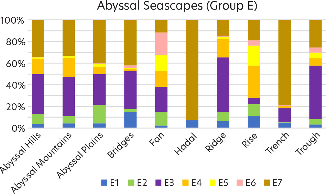
FIGURE 10. The distribution of geomorphic features by seascape as a percent of area is plotted in this bar graph. > High res figure

 

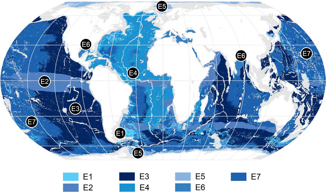
FIGURE 11. Map shows the locations of seascapes E1 to E7 that characterize the abyssal to hadal ocean floor. > High res figure

 

Plateaus (Group F)

Multivariate analysis of the ocean floor having plateaus identified seven separate seascapes (Figure 12). Distinguishing and unique aspects that characterize plateau seascapes are as follows:

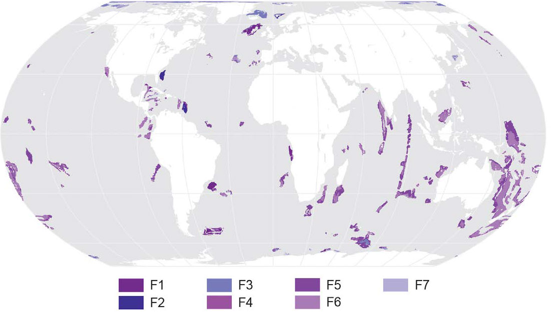
• F1 – 6.4% of plateau seascapes by area, has the greatest mean sediment thickness of 4,168 m, located mainly in the Atlantic Ocean.
• F2 – 1.6% of plateau seascapes by area, has very strong maximum bottom current speed of 0.44 m s^–1 (nearly equal to F9), comprised of two plateaus located in the western Atlantic and one plateau off Norway. F2 has the lowest heterogeneity among plateau seascapes of 0.12 polygons per 1,000 km².
• F3 – 8.0% of plateau seascapes by area, has the most alkaline mean bottom water pH of 8.02, located mainly in the Arctic Ocean and the North Atlantic.
• F4 – 6.9% of plateau seascapes by area, deepest plateaus at mean depth of 3,074 m, lowest (most acidic) pH of 7.81, thinnest mean sediment cover of 518 m, broadly distributed but mainly located in the Pacific and Indian Oceans.
• F5 – 34.9% of plateau seascapes by area, the largest seascape by area, similar to F4 as it is broadly distributed but mainly located in the Pacific and Indian Oceans.
• F6 – 33.0% of plateau seascapes by area, has the lowest mean dissolved oxygen level of 156 mmol m^–³, broadly distributed.
• F7 – 1.1% of plateau seascapes, the smallest plateau seascape by area, steepest seafloor gradient of 5.08°, coldest mean bottom water temperature of –0.5°C, and lowest mean POC flux of 0.01 mmol/m²/d, located mainly in the Arctic and Southern Oceans. F7 has the greatest heterogeneity of 8.85 polygons per 1,000 km² (highest of all seascapes, globally).
• F8 – 3.4% of plateau seascapes by area, most gentle seafloor slope of 0.39°, most shallow mean depth of 530 m, warmest mean bottom water temperature of 7.34°C, greatest mean POC flux of 1.87 mmol/m²/d, located mainly adjacent to New Zealand.
• F9 – 4.8% of plateau seascapes by area, has very strong maximum bottom current speed of 0.46 m s^–1 (compare to F2), broadly distributed.

 

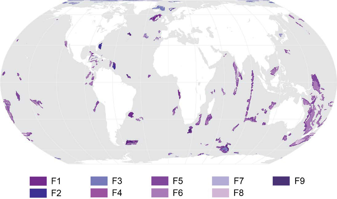
FIGURE 12. Seascapes F1 to F9 that characterize plateaus are plotted here. > High res figure

 

Results: Ecological Benthic Units

The individual polygons located within specific geomorphic feature polygons are termed ecological benthic units (EBUs). Each EBU is a unique combination of a biophysical (bottom water) seascape located within a particular geomorphic unit. A total of 697,235 EBUs have been identified in this study.

The characteristics of EBUs provide specific environmental context for the geomorphic feature in which they occur and provide a basis for distinguishing between features of the same type (i.e., differences among seamounts, submarine canyons, and deep ocean trenches). The information can be accessed through the online EBU Explorer created as an output of this project. The following section provides examples of specific geomorphic features and the EBUs they contain.

 

“The Gully” Submarine Canyon

“The Gully” submarine canyon, located about 200 km off the coast of Nova Scotia, Canada, is 15–16 km wide and extends approximately 65 km downslope to a depth of over 3,000 m. It is a shelf-​incising canyon carved into Tertiary bedrock draped by Quaternary glaciomarine sediments. The canyon was formed by combined mass wasting of the slope and turbidity currents during the Pleistocene. The Gully links the shallow banks of the continental shelf with deeper, steep canyon walls that support cold-water corals and other benthic fauna, while the canyon floor supports deep-water fish, invertebrates, and deep-diving cetaceans, linking surface, pelagic, and benthic ecosystems (Harrison and Fenton, 1998; Fisheries and Oceans Canada, 2025).

Figure 13 shows screenshots of information provided by the EBU Explorer tool for The Gully canyon. The dialogue box indicates that the highlighted feature is a shelf-incising submarine canyon and that there are 20 EBUs within the canyon polygon. The bar graph illustrates how The Gully compares globally with shelf-incising submarine canyons, indicating that The Gully has a relatively high proportion of seascape B3, with oxygen-rich waters. In contrast, there is an absence of seascapes B4, B5, and B9.

The panels below the bar graph contain information on the 20 EBUs, listed in order of decreasing percent area. The top EBU number, 157859 (seascape B3), covers 75.2% of The Gully, and it is located mainly on the lower continental slope. The second EBU number, 161480 (seascape B7), covers 10.2% of The Gully and is located mainly on the upper continental slope and across the shelf break. EBU B7 is 1°C warmer in mean temperature than B3 (4.4°C versus 3.4°C), illustrating the most significant difference in physical properties between the two (Figure 13).

 

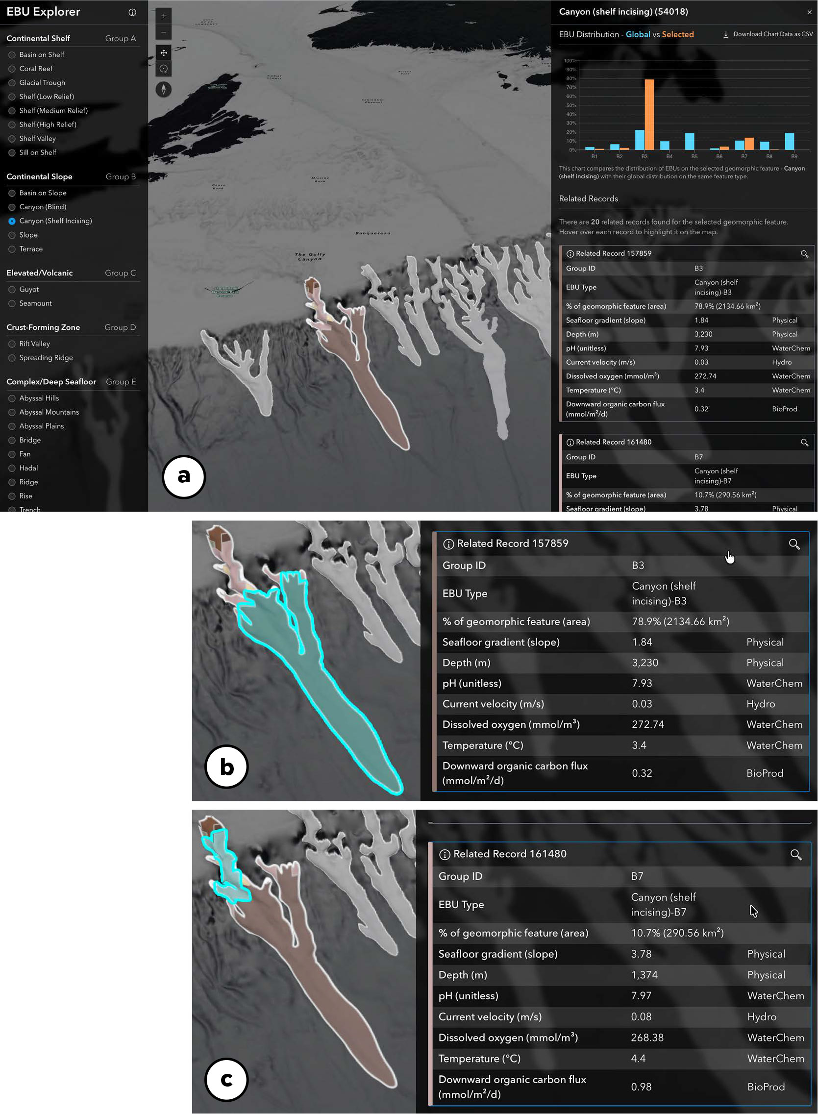
FIGURE 13. Screenshots taken from the EBU Explorer show the The Gully submarine canyon off Newfoundland, Canada. (a) Location of The Gully with bar graph showing the relative proportion of EBUs characterizing all shelf-​incising canyons (in blue) versus the EBUs that characterize The Gully canyon (in orange). (b) Zoom-in view of EBU B3 with respective information panel. (c) Zoom-in view of EBU B7. > High res figure

 

Mariana Trench

The Mariana Trench, the deepest part of the ocean, is located in the western Pacific Ocean, east of the Mariana Islands. It forms a long, narrow, crescent-shaped depression created where the Pacific Plate subducts beneath the smaller Philippine Sea Plate and the small, crescent-shaped Mariana microplate that broke off from it (van Rijsingen, 2019). It is ~2,500 km in length, 70–100 km in width, and reaches its deepest point at 10,935 m in the Challenger Deep (Greenaway et al., 2021). The Trench has steep, asymmetric sides, and the western wall is typically steeper due to tectonic forces that include the large age differential between the down­going and overriding plates.

Figure 14 shows a segment of the Mariana Trench illustrating its composition relative to trenches globally. Seascape E7 is dominant in most trenches, as it is with the Mariana Trench, characterized by cold temperatures and acidic bottom waters (see also Figure 10). But in contrast to other trenches, the Mariana Trench does not contain any area of seascapes E2, E3, E4, or E6 (Figure 14).

 

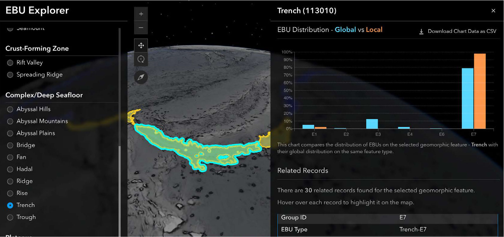
FIGURE 14. Screenshot taken from the EBU Explorer showing a section of the Mariana Trench in the Pacific Ocean. The bar graph plots the relative proportion of EBUs comprising the trench, which is dominated by seascape E7; seascape E1 covers less than 2%. The largest EBU, which covers 60.3% of the trench, is shown here. > High res figure

 

Gifford Guyot

Gifford Guyot is a flat-topped seamount located on the Lord Howe Rise plateau in the Coral Sea. The Gifford Marine Park is included within the Australian Government’s national marine protected area network (Nanson et al., 2018). The Guyot formed as the Indo-Australian plate migrated north across a stationary magma source (“hotspot”) during the Middle Miocene (about 15 million years ago) and has a depth range of approximately 3 km, rising from 3,400 m on the abyssal plain to as shallow as 250 at its summit (Nanson et al., 2018).

Figure 15 illustrates the dominance of seascape C5, characterized by warm water temperatures around the Gifford Guyot. In contrast, most guyots globally are dominated by seascape C4 with its colder water temperatures. Of particular significance is the above-average occurrence of seascape C3 on the Gifford since this seascape was noted above for its high heterogeneity and high potential for benthic productivity and biomass. Limited sampling of the Gifford suggests the presence of a relatively diverse, albeit sparse, epibenthic assemblage, including mixed cold-water coral and sponge assemblages (Nanson et al., 2018).

 

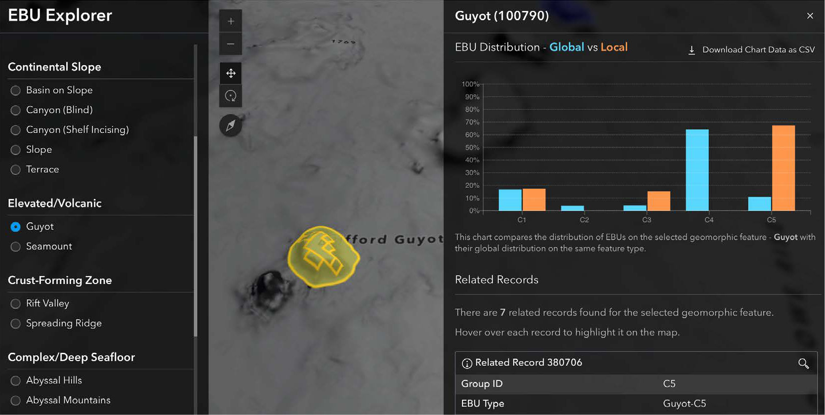
FIGURE 15. Screenshot taken from the EBU Explorer describes Gifford Guyot in the Coral Sea. The bar graph shows the relative proportion of EBUs comprising Gifford Guyot, which is dominated by seascape C5. > High res figure

 

Discussion

Insights into Global Benthic Biodiversity from EBUs

The diversity of EBUs is an indicator of the diversity found in benthic ecosystems, and as such, it can also be considered to represent benthic biodiversity in terms of likely species richness for a given area (e.g., Harris and Baker, 2020; Almond et al., 2021; Girard et al., 2025). Our map of EBU heterogeneity (Figure 16) has direct applications in designing and cross-validating spatial conservation zones (i.e., marine protected areas, MPAs; Howell, 2010; Fischer et al., 2019); we note, for example, the close correspondence between our map of EBU diversity (Figure 16) and the map of MPA prioritized areas by Zhao et al. (2020, their Figure 4). The hotspots of heterogeneity (Figure 16) immediately suggest themselves within bioregions as candidates for MPAs, where the maximum biodiversity can be conserved in the smallest possible area (Roff and Taylor, 2000). They are also areas where targeted marine surveys could be optimized to investigate the regional diversity of environments.

 

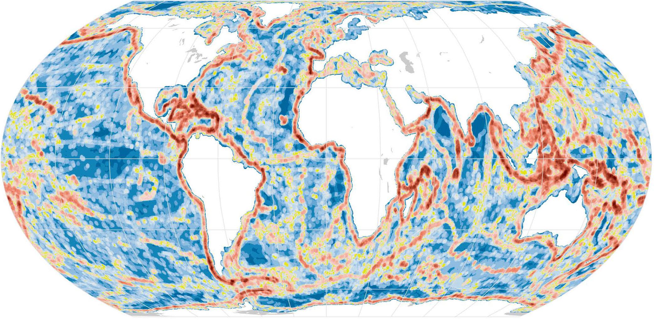
FIGURE 16. Map showing the heterogeneity of the global ocean based on focal variety analysis of EBU polygons within a 100 km search radius. Blue colors indicate heterogeneities as low as 1 and red colors heterogeneities as high as 50. Higher heterogeneity values identify broad transition zones where multiple EBU types occur together within a regional neighborhood. > High res figure

 

CCD and Acidification

EBUs provide the first global, spatially explicit view of how seafloor habitats are distributed relative to the CCD and therefore quantify which benthic systems are already exposed—or will soon be exposed—to corrosive, low-pH bottom waters. Seascape E7, the most abundant seascape globally (95.6 million km²), is characterized by a mean pH of 7.75, already below the modern CCD threshold used in this study. The extent of E7 highlights that a substantial fraction of the global abyss is currently bathed in waters corrosive to calcium carbonate (CaCO₃). This has direct ecological implications: the CCD has recently been demonstrated to act as a biological boundary that structures abyssal biogeography (Simon-Lledó et al., 2023), and experimental studies confirm that decreasing pH reduces fitness and survival in several abyssal taxa (Barry et al., 2013).

As the ocean continues to absorb anthropogenic CO₂, deep-​water masses entering the global conveyor belt (thermohaline circulation system) will carry progressively lower pH and oxygen concentrations. Model and observational evidence indicate that the CCD is rising (Sulpis et al., 2018; Harris et al., 2023), resulting in increasing areas of the seafloor—particularly in older, sediment-​starved basins—crossing into undersaturated conditions. EBUs therefore allow us to identify which geomorphic systems lie nearest to this chemical boundary and where upward shoaling of the CCD will most rapidly expose carbonate-dependent habitats and fauna to corrosive conditions.

EBUs offer a novel geospatial tool for quantifying ecosystem vulnerability to ocean acidification by mapping the intersection of benthic environments, geomorphic features, and evolving carbonate saturation horizons. This capability is directly relevant to global MPA planning, environmental impact assessment for deep-sea industries, and future biodiversity monitoring frameworks.

 

Oxygen Dead Zones

Oxygen minimum zones (OMZs) are expanding globally due to warming-driven stratification and reduced ventilation, and EBUs provide a new way to map where low-oxygen waters intersect specific geomorphic settings. Slope seascapes B1 and B5 represent the clearest expression of this phenomenon: they contain hypoxic (72.2 mmol m^–³) and severely hypoxic (52.5 mmol m^–³) bottom waters, respectively, and together cover 4.16 million km². Their distribution—along the continental margins of the Pacific Rim, western South America, North America, and parts of Asia, Africa, India, New Zealand, and Tasmania—closely matches known global OMZ cores (Paulmier and Ruiz-Pino, 2009).

These oxygen-depleted environments (oxygen dead zones) have well-documented ecological consequences, including reduced habitat suitability for metabolically sensitive taxa, compression of species’ depth ranges, altered trophic structure, and enhanced vulnerability of demersal fisheries (Diaz and Rosenberg, 2008; Levin, 2018). Our results show that the most oxygen-stressed systems (and EBUs) occur on economically important slopes near productive shelf ecosystems, where many nations rely on fisheries resources.

The ability to quantify the areal extent and geomorphic context of hypoxic EBUs provides a practical tool for evaluating where deepening OMZs will next make contact with slope habitats, and which regions are most at risk of biodiversity loss or fisheries displacement. As oxygen minimum zones continue to intensify under climate change (Grégoire et al., 2021), EBUs offer a globally consistent spatial framework for monitoring, forecasting, and prioritizing management responses.

 

Seamount Habitat and Conservation Priorities

Seamounts and guyots host some of the most ecologically distinctive habitats in the deep ocean, yet they vary enormously in their environmental conditions and biodiversity potential (Rogers, 2000; Clark et al., 2011). EBUs allow these differences to be quantified globally for the first time. Among the five seamount and guyot seascapes, C3 stands out as a rare and highly favorable habitat type, combining warm, oxygenated bottom waters (mean 185 mmol m^–³ dissolved oxygen), relatively strong currents, elevated POC flux, and pH values above the CCD. Together, these conditions promote enhanced suspension-feeding communities, greater metabolic scope for fauna, and increased ecological connectivity. Despite its favorable characteristics, C3 is extremely limited in extent, representing <1% of global seamount and guyot area. We note also that favorable environmental conditions may not always equate with higher biodiversity. While we can define relatively rare habitats, we cannot be certain that they are host to an especially unique community.

By contrast, the majority of seamounts occur within C2, C4, and C5, which are characterized by cold, low-productivity, low-POC-flux waters—conditions associated with sparse benthic assemblages and reduced potential for habitat-forming taxa such as corals and sponges. This global environmental pattern suggests that the vast majority of seamounts reside in ecological “cold spots,” while a very small minority form important biodiversity reservoirs. The EBU framework therefore highlights two conservation priorities: (1) recognition of naturally rare, highly productive seamount habitats (e.g., C3 units) as critical areas for biodiversity protection, ecological monitoring, and potential MPA designation within a network of ecologically representative areas (Zhao et al. 2020); and (2) differentiation among superficially similar seamounts—​allowing managers to move beyond treating all seamounts as equivalent, which has historically hindered ecologically representative and coherent conservation planning.

These insights align with previous biogeographic analyses demonstrating that seamounts cannot be managed as a single class of features. Clark et al. (2011), for example, identified 194 distinct seamount classes based on oxygen, depth, production regimes, and geographic context, and demonstrated their ecological relevance by comparing classes with distributions of octocoral assemblages. EBUs extend this approach globally and at higher spatial resolution, enabling direct integration of geomorphology, environmental regimes, and carbonate chemistry into conservation decision-making.

For high-seas MPA planning, fisheries management, and general ocean human-use and infrastructure management, EBUs therefore provide a transformative tool: they identify which seamounts host rare ecological configurations, which are exposed to hypoxia or acidification, and which exist within areas less suitable for benthic life. This differentiation is essential for prioritizing surveys, assigning conservation value, and evaluating the vulnerability of seamount systems in a rapidly changing ocean.

 

Conclusion

This study presents the first global benthic classification system that explicitly integrates seafloor geomorphology with environmental regimes to generate 250 unique EBUs distributed on the seafloor as nearly 700,000 EBU polygon occurrences. By combining geomorphic structure with key biophysical drivers—including temperature, oxygen, pH, carbon flux, bottom currents, and sediment thickness—the EBU framework reveals previously unrecognized environmental gradients and boundaries across the global ocean floor.

EBUs demonstrate that benthic habitats are far more heterogeneous than suggested by geomorphology or environmental variables alone. The resulting classification highlights important environmental patterns: the dominance of CCD-exposed abyssal plains (E7), the concentration of hypoxic environments along productive continental margins (B1, B5), and the extreme rarity of seamounts with high biodiversity potential (C3). These patterns underscore the uneven distribution of environmental vulnerability across the seafloor and show how different geomorphic settings mediate exposure to climate stressors such as acidification, deoxygenation, and shifting food supply.

As a global characterization of the seafloor for decision support, EBUs have direct application to high-seas MPA design, national assessments of the representativeness of MPA networks, environmental impact assessments, and biodiversity baseline proxies for emerging conservation frameworks under the UN High Seas Treaty, and more. Because EBUs operate at the scale of geomorphic features that are widely used in marine policy, they provide an intuitive and spatially resolved way to compare habitats within and among ocean basins, identify rare or vulnerable systems, and guide prioritization for exploration and protection. The ocean is vast, and grossly under-sampled. EBUs can help target exploration and sampling efforts by providing a framework for the design of a global sampling strategy.

While the present analysis offers the most comprehensive global benthic classification to date, further refinements will benefit from time-varying environmental datasets, higher-resolution bathymetry, and expanded biological observations to strengthen ecological validation. In this study we have delineated what we believe to be ecologically meaningful areas, but further study is needed to more fully understand the relationship between our complexes of unique physical environments and actual species distributions. As new global datasets emerge, EBUs can be dynamically updated, providing a living framework for monitoring environmental change in the deep sea. They may also provide a useful extension to the General Bathymetric Chart of the Oceans (GEBCO) grid of the UN Nippon Foundation–GEBCO Seabed 2030 program (Mayer et al., 2018), lending insight into the EBUs beyond just bathymetry.

In summary, EBUs offer a transformative step forward for global ocean management by linking where benthic habitats occur, what environmental regimes define them, and how vulnerable they are to future change. This integrative approach delivers a foundation for more informed and proactive stewardship of the world’s largest, least understood biome. As a reproducible, data-driven, and updatable global classification, EBUs deliver a new decision-support resource that helps to power area-based management tools for understanding and managing the world’s largest and least explored biome.

 

Acknowledgments

The authors appreciate the helpful comments from Mark Wiltermuth (U.S. Geological Survey) and the insights of three anonymous reviewers. Any use of trade, firm, or product names is for descriptive purposes only and does not imply endorsement by the U.S. Government. We thank Esri for in-kind computational support and Andrew Skinner for additional cartographic help with Figures 1–2, 4–6, 8–9, 11–12, and 16. P.T.H., D.J.W., R.S., K.H., G.K., and M.J.C. participated in an introductory workshop to design the research; P.T.H., K.B., K.V., and D.J.W. performed the research; K.B. and K.V. analyzed the data and prepared the figures; K.V. developed the web app; and P.T.H., D.J.W., K.B., K.V., M.J.C., K.H., G.K., V.L., M.M.-L., and R.S. wrote the paper. The authors declare no competing interest.

Harris, P.T., D.J. Wright, K. Butler, K. VanGraafeiland, M.J. Costello, K. Howell, G. Kågesten, V. Lucieer, M. Macmillan-Lawler, and R. Sayre. 2026. Ecological benthic units (EBUs): A new characterization of the global seafloor for ocean spatial planning and management. Oceanography 39(2):17–33, https://doi.org/10.5670/oceanog.2026.e211.

Table S1

1. Almond, P.M., K. Linse, S. Dreutter, S.M. Grant, H.J. Griffiths, R.J. Whittle, M. Mackenzie, and W.D.K. Reid. 2021. In-situ image analysis of habitat heterogeneity and benthic biodiversity in the Prince Gustav Channel, Eastern Antarctic Peninsula. Frontiers in Marine Science 8:614496, https://doi.org/10.3389/fmars.2021.614496.
2. Assis, J., S.J. Fernández Bejarano, V.W. Salazar, L. Schepers, L. Gouvêa, E. Fragkopoulou, F. Leclercq, B. Vanhoorne, L. Tyberghein, and E.A. Serrão. 2024. Bio-ORACLE v3. 0: Pushing marine data layers to the CMIP6 Earth System Models of climate change research. Global Ecology and Biogeography 33(4):e13813, https://doi.org/10.1111/geb.13813.
3. Astudillo-Scalia, Y., F. Albuquerque, B. Polidoro, and P. Beier. 2021. Environmental diversity as a reliable surrogacy strategy of marine biodiversity. Perspectives in Ecology and Conservation 19(2021):429–434, https://doi.org/10.1016/j.pecon.​2021.08.002.
4. Baker, E.K., K. Thygesen, and P.T. Harris. 2024. Increase in Oxygen Depletion in the Marine Environment: Drivers and Recommendations. Arendal, Norway, GRID-Arendal, 32 pp., https://grid-arendal.herokuapp.com/publications/1034.
5. Barry, J.P., K.R. Buck, C. Lovera, P.G. Brewer, B.A. Seibel, J.C. Drazen, M.N. Tamburri, P.J. Whaling, L. Kuhnz, and E.F. Pane. 2013. The response of abyssal organisms to low pH conditions during a series of CO₂-release experiments simulating deep-sea carbon sequestration. Deep Sea Research Part II 92:249–260, https://doi.org/​10.1016/j.dsr2.2013.03.037.
6. Baynes, T., and A. Szmant. 1989. Effect of current on the sessile benthic community structure of an artificial reef. Bulletin of Marine Science 44:545–566.
7. Becker, J.J., D.R. Sandwell, W.H.F. Smith, J. Braud, B. Binder, J. Depner, D. Fabre, J. Factor, S. Ingalls, S.H. Kim, and others. 2009. Global bathymetry and elevation data at 30 arc seconds resolution: SRTM30_PLUS. Marine Geodesy 32(4):355–371, https://doi.org/10.1080/01490410903297766.
8. Bisson, K., H. McMonagle, I. Iglesias, S. Halfter, and N. Gallo. 2023. Five reasons to take the precautionary approach to deep sea exploitation. Communications Earth & Environment 4(1):152, https://doi.org/10.1038/s43247-023-00823-4.
9. Breitburg, D.L., D.W. Hondorp, L.A. Davias, and R.J. Diaz. 2009. Hypoxia, nitrogen, and fisheries: Integrating effects across local and global landscapes. Annual Review of Marine Science 1(1):329–349, https://doi.org/10.1146/annurev.marine.010908.163754.
10. Brodeau, L., B. Barnier, A.M. Treguier, T. Penduff, and S. Gulev. 2010. An ERA40-based atmospheric forcing for global ocean circulation models. Ocean Modelling 31:88–104, https://doi.org/​10.1016/j.ocemod.2009.10.005.
11. Capotondi, A., R.R. Rodrigues, A. Sen Gupta, J.A. Benthuysen, C. Deser, T.L. Frölicher, N.S. Lovenduski, D.J. Amaya, N. Le Grix, T. Xu, and others. 2024. A global overview of marine heatwaves in a changing climate. Communications Earth & Environment 5(1):701, https://doi.org/10.1038/s43247-024-01806-9.
12. Ceccarelli, D.M., K. Davey, G.P. Jones, P.T. Harris, S.V. Matoto, J. Raubani, and L. Fernandes. 2021. How to meet new global targets in the offshore realms: Biophysical guidelines for offshore networks of no-take marine protected areas. Frontiers in Marine Science 8:634574, https://doi.org/10.3389/fmars.2021.634574.
13. Chavez, F.P., and M. Messié. 2009. A comparison of eastern boundary upwelling ecosystems. Progress in Oceanography 83(1):80–96, https://doi.org/10.1016/​j.pocean.2009.07.032.
14. Clark, M.R., L. Watling, C. Smith, A. Rowden, and J.M. Guinotte. 2011. A global seamount classification to aid the scientific design of marine protected area networks. Ocean & Coastal Management 54(1):19–36, https://doi.org/10.1016/​j.ocecoaman.2010.10.006.
15. Costello, M.J., R. Corkrey, A.E. Bates, M.T. Burrows, C. Chaudhary, G.C. Edgar, R.D. Stuart-Smith, M. Yasuhara, and C.-L. Wei. 2023. The universal evolutionary and ecological significance of 20°C. Frontiers of Biogeography 15(4):e61673, https://doi.org/​10.21425/F5FBG61673.
16. Diaz, R.J., and R. Rosenberg. 2008. Spreading dead zones and consequences for marine ecosystems. Science 321(5891):926–929, https://doi.org/10.1126/science.1156401.
17. Fischer, A., D. Bhakta, M. Macmillan-Lawler, and P.T. Harris. 2019. Existing global marine protected area network is not representative or comprehensive measured against seafloor geomorphic features and benthic habitats. Ocean & Coastal Management 167:176–187, https://doi.org/10.1016/j.ocecoaman.2018.10.001.
18. Fisheries and Oceans Canada (DFO). 2025. “The Gully Marine Protected Area.” Government of Canada, https://www.dfo-mpo.gc.ca/oceans/mpa-zpm/gully/index-eng.html.
19. FES Tide Product. 2022. The FES2022 Tide product was funded by CNES, produced by LEGOS, NOVELTIS and CLS and made freely available by AVISO. CNES, 2024. FES2022 (Finite Element Solution) Ocean Tide (Version 2022) [Data set], CNES, https://doi.org/10.24400/527896/A01-2024.004
20. Gage, J.D., and P.A. Tyler. 1991. Deep-Sea Biology: A Natural History of Organisms at the Deep-Sea Floor. Cambridge University Press, Cambridge, 504 pp., https://doi.org/​10.1017/CBO9781139163637.
21. Girard, F., D.W. Caress, J.B. Paduan, L.A. Kuhnz, S.Y. Litvin, E. Flattery, A.S. Kahn, A. DeVogelaere, E.J. Burton, C. Lovera, and others. 2025. Habitat heterogeneity over multiple scales supports dense and diverse megafaunal communities on a northeast Pacific ridge. Limnology and Oceanography 70(2):377–392, https://doi.org/​10.1002/lno.12766.
22. Greenaway, S.F., K.D. Sullivan, S.H. Umfress, A.B. Beittel, and K.D. Wagner. 2021. Revised depth of the Challenger Deep from submersible transects; including a general method for precise, pressure-derived depths in the ocean. Deep Sea Research Part I 178:103644, https://doi.org/10.1016/j.dsr.2021.103644.
23. Grégoire, M., V. Garçon, H. Garcia, D. Breitburg, K. Isensee, A. Oschlies, M. Telszewski, A. Barth, H.C. Bittig, J. Carstensen, and others. 2021. A global ocean oxygen database and atlas for assessing and predicting deoxygenation and ocean health in the open and coastal ocean. Frontiers in Marine Science 8:724913, https://doi.org/​10.3389/fmars.2021.724913
24. Harris, P.T., and T. Whiteway. 2009. High seas marine protected areas: Benthic environmental conservation priorities from a GIS analysis of global ocean biophysical data. Ocean and Coastal Management 52:22–38, https://doi.org/10.1016/​j.ocecoaman.2008.09.009.
25. Harris, P.T. 2012. Biogeography, benthic ecology, and habitat classification schemes. Pp. 61–91 in Seafloor Geomorphology as Benthic Habitat: GeoHab Atlas of Seafloor Geomorphic Features and Benthic Habitats. P.T. Harris and E.K. Baker, eds, Elsevier, Amsterdam, https://doi.org/10.1016/B978-0-12-385140-6.00004-9.
26. Harris, P.T., M. MacMillan-Lawler, J. Rupp, and E.K. Baker. 2014. Geomorphology of the oceans. Marine Geology 352:4–24, https://doi.org/10.1016/j.margeo.2014.01.011.
27. Harris, P.T., and E.K. Baker, eds. 2020. Seafloor Geomorphology as Benthic Habitat: GeoHab Atlas of Seafloor Geomorphic Features and Benthic Habitats. 2nd ed., Elsevier, Amsterdam, 1,076 pp., https://doi.org/10.1016/B978-0-12-814960-7.00060-9.
28. Harris, P.T., L. Westerveld, Q. Zhao, and M.J. Costello. 2023. Rising snow line: Ocean acidification and the submergence of seafloor geomorphic features beneath a rising carbonate compensation depth. Marine Geology 463:107121, https://doi.org/​10.1016/j.margeo.2023.107121.
29. Harrison, W.G., and D.G. Fenton, eds. 1998. The Gully: A Scientific Review of Its Environment and Ecosystem. Canadian Technical Report of Fisheries and Aquatic Sciences 2245. Fisheries and Oceans Canada, Dartmouth, Nova Scotia, 282 pp.
30. High Seas Alliance. 2025. “High Seas Treaty Ratification Tracker,” https://highseasalliance.org/treaty-ratification/.
31. Howell, K.L. 2010. A benthic classification system to aid in the implementation of marine protected area networks in the deep/high seas of the NE Atlantic. Biological Conservation 143(5):1,041–1,056, https://doi.org/10.1016/j.biocon.2010.02.001.
32. Huang, B., C. Liu, V. Banzon, E. Freeman, G. Graham, B. Hankins, T. Smith, and H.-M. Zhang. 2021. Improvements of the Daily Optimum Interpolation Sea Surface Temperature (DOISST) Version 2.1. Journal of Climate 34:2,923–2,939, https://doi.org/​10.1175/JCLI-D-20-0166.1
33. Juniper, S.K., M. Matabos, S. Mihaly, R.S. Ajayamohan, F. Gervais, and A.O.V. Bui. 2013. A year in Barkley Canyon: A time-series observatory study of mid-slope benthos and habitat dynamics using the NEPTUNE Canada network. Deep Sea Research Part II 92:114–123, https://doi.org/10.1016/j.dsr2.2013.03.038.
34. Levin, L.A. 2018. Manifestation, drivers, and consequences of ocean deoxygenation. Annual Review of Marine Science 10:229–260, https://doi.org/10.1146/annurev-marine-121916-063359.
35. Mayer, L., M. Jakobsson, G. Allen, B. Dorschel, R. Falconer, V. Ferrini, G. Lamarche, H. Snaith, and P. Weatherall. 2018. The Nippon Foundation—GEBCO Seabed 2030 Project: The quest to see the world’s oceans completely mapped by 2030. Geosciences 8(2):63, https://doi.org/10.3390/geosciences8020063.
36. McArthur, M., B. Brooke, R. Przeslawski, D. Ryan, V. Lucieer, S. Nichol, A. McCallum, C. Mellin, I. Cresswell, and L. Radke. 2010. On the use of abiotic surrogates to describe marine benthic biodiversity. Estuarine, Coastal and Shelf Science 88(1):21–32, https://doi.org/10.1016/j.ecss.2010.03.003.
37. McQuaid, K.A., A.E.H. Bridges, K.L. Howell, T.B.R. Gandra, V. de Souza, J.C. Currie, O.T. Hogg, T.R.R. Pearman, J.B. Bell, L.J. Atkinson, and others. 2023. Broad-scale benthic habitat classification of the South Atlantic. Progress in Oceanography 214:103016, https://doi.org/10.1016/j.pocean.2023.103016.
38. Misiuk, B., and C.J. Brown. 2024. Benthic habitat mapping: A review of three decades of mapping biological patterns on the seafloor. Estuarine, Coastal and Shelf Science 296:108599, https://doi.org/10.1016/j.ecss.2023.108599.
39. Muller, R.D., M. Sdrolias, C. Gaina, and W.R. Roest. 2008. Age, spreading rates, and spreading symmetry of the world’s ocean crust. Geochemistry, Geophysics and Geosystems 9(4), https://doi.org/10.1029/2007GC001743.
40. Nanson, R., A. Carroll, Z. Huang, S. Nichol, and K. Miller. 2018. An Eco-Narrative of Gifford Marine Park: Temperate East Marine Region. Report to the National Environmental Science Programme, Marine Biodiversity Hub, Geoscience Australia Canberra, 17 pp.
41. Olson, P., E. Reynolds, L. Hinnov, and A. Goswami. 2016. Variation of ocean sediment thickness with crustal age. Geochemistry, Geophysics, Geosystems 17(4), https://doi.org/​10.1002/2015GC006143.
42. Paulmier, A., and D. Ruiz-Pino. 2009. Oxygen minimum zones (OMZs) in the modern ocean. Progress in Oceanography 80(3–4):113–128, https://doi.org/10.1016/​j.pocean.2008.08.001.
43. Ramirez-Llodra, E., P.A. Tyler, M.C. Baker, O.A. Bergstad, M.R. Clark, E. Escobar, L.A. Levin, L. Menot, A.A. Rowden, C.R. Smith, and C.L. Van Dover. 2011. Man and the last great wilderness: Human impact on the deep sea. PLoS ONE 6(8):e22588, https://doi.org/10.1371/journal.pone.0022588.
44. Richter, M.E., K.J. Heywood, R.A. Hall, and P.E. Davis. 2025. Observations of turbulent mixing in the Dotson Ice Shelf cavity. Ocean Science 21:3,341–3,359, https://doi.org/​10.5194/os-21-3341-2025.
45. Riehl, T., A.-C. Wölfl, N. Augustin, C.W. Devey, and A. Brandt. 2020. Discovery of widely available abyssal rock patches reveals overlooked habitat type and prompts rethinking deep-sea biodiversity. Proceedings of the National Academy of Sciences of the United States of America 117(27):15,450–15,459, https://doi.org/10.1073/pnas.1920706117.
46. Roff, J.C., and M.E. Taylor. 2000. National frameworks for marine conservation – A hierarchical geophysical approach. Aquatic Conservation: Marine and Freshwater Ecosystems 10:209–223, https://doi.org/​10.1002/​1099-0755​(200005/06)10:3<209::AID-AQC408>3.0.CO;2-J.
47. Rogers, A.D. 2000. The role of the oceanic oxygen minima in generating biodiversity in the deep sea. Deep-Sea Research Part II 47:119–148, https://doi.org/10.1016/S0967-0645(99)00107-1
48. Romoth, K., A. Darr, S. Papenmeier, M.L. Zettler, and M. Gogina. 2023. Substrate heterogeneity as a trigger for species diversity in marine benthic assemblages. Biology 12(6):825, https://doi.org/10.3390/biology12060825.
49. Sayre, R.G., D.J. Wright, S.P. Breyer, K.A. Butler, K. VanGraafeiland, M.J. Costello, P.T. Harris, K.L. Goodin, J.M. Guinotte, Z. Basher, and others. 2017. A three-​dimensional mapping of the ocean based on environmental data. Oceanography 30(1):90–103, https://doi.org/10.5670/oceanog.2017.116.
50. Simon-Lledó, E., D.J. Amon, G. Bribiesca-Contreras, D. Cuvelier, J.M. Durden, S.P. Ramalho, K. Uhlenkott, P.M. Arbizu, N. Benoist, J. Copley, and others. 2023. Carbonate compensation depth drives abyssal biogeography in the northeast Pacific. Nature Ecology & Evolution 7(9):1,388–1,397, https://doi.org/10.1038/s41559-023-02122-9.
51. Smith, C.R., F.C. De Leo, A.F. Bernardino, A.K. Sweetman, and P.M. Arbizu. 2008. Abyssal food limitation, ecosystem structure and climate change. Trends in Ecology & Evolution 23(9):518–528, https://doi.org/10.1016/j.tree.2008.05.002.
52. Straume, E.O., C. Gaina, S. Medvedev, K. Hochmuth, K. Gohl, J.M. Whittaker, R. Abdul Fattah, J.C. Doornenbal, and J.R. Hopper. 2019. GlobSed: Updated total sediment thickness in the world’s oceans. Geochemistry, Geophysics, Geosystems 20(4):1,756–1,772, https://doi.org/10.1029/2018GC008115.
53. Stuart-Smith, R.D., G.J. Edgar, and A.E. Bates. 2017. Thermal limits to the geographic distributions of shallow-water marine species. Nature Ecology & Evolution 1:1,846–1,852, https://doi.org/10.1038/s41559-017-0353-x.
54. Sulpis, O., B.P. Boudreau, A. Mucci, C. Jenkins, D.S. Trossman, B.K. Arbic, and R.M. Key. 2018. Current CaCO₃ dissolution at the seafloor caused by anthropogenic CO₂. Proceedings of the National Academy of Sciences of the United States of America 115(46):11,700–11,705, https://doi.org/10.1073/pnas.1804250115.
55. Sweetman, A.K., A.J. Smith, D.S.W. de Jonge, T. Hahn, P. Schroedl, M. Silverstein, C. Andrade, R.L. Edwards, A.J.M. Lough, C. Woulds, and others. 2024. Evidence of dark oxygen production at the abyssal seafloor. Nature Geoscience 17(8):737–739, https://doi.org/10.1038/s41561-024-01480-8.
56. Tibshirani, R., G. Walther, and T. Hastie. 2001. Estimating the number of clusters in a data set via the gap statistic. Journal of the Royal Statistical Society: Series B 63(2):411–423, https://doi.org/10.1111/1467-9868.00293.
57. US FGDC (United States Federal Geographic Data Committee). 2012. Coastal and Marine Ecological Classification Standard (CMECS) (FGDC-STD-018-2012). National Oceanic and Atmospheric Administration (NOAA), Washington, DC, 353 pp., https://repository.library.noaa.gov/view/noaa/27552.
58. van Rijsingen, E., F. Funiciello, F. Corbi, and S. Lallemand. 2019. Rough subducting seafloor reduces interseismic coupling and mega-earthquake occurrence: Insights from analogue models. Geophysical Research Letters 46(6):3,124–3,132, https://doi.org/​10.1029/2018GL081272.
59. Woodgate, R.A., and E. Fahrbach. 1999. Benthic storms in the Greenland Sea. Deep Sea Research Part I 46(12):2,109–2,127, https://doi.org/10.1016/S0967-​0637(99)00037-0.
60. Zeppilli, D., A. Pusceddu, F. Trincardi, and R. Danovaro. 2016. Seafloor heterogeneity influences the biodiversity-ecosystem functioning relationships in the deep sea. Scientific Reports 6(1):26352, https://doi.org/10.1038/srep26352.
61. Zhao, Q., F. Stephenson, C. Lundquist, K. Kaschner, D.R.M. Jayathilake, and M.J. Costello. 2020. Where marine protected areas would best represent 30% of ocean biodiversity. Biological Conservation 244:108536, https://doi.org/10.1016/​j.biocon.2020.108536.

This is an open access article made available under the terms of the Creative Commons Attribution 4.0 International License (https://creativecommons.org/licenses/by/4.0/), which permits use, sharing, adaptation, distribution, and reproduction in any medium or format as long as users cite the materials appropriately, provide a link to the Creative Commons license, and indicate the changes that were made to the original content. Images, animations, videos, or other third-party material used in articles are included in the Creative Commons license unless indicated otherwise in a credit line to the material. If the material is not included in the article’s Creative Commons license, users will need to obtain permission directly from the license holder to reproduce the material.