PURPOSE OF ACTIVITY

This guided, inquiry-based, hands-on lesson uses data from a local monitoring station in Tampa Bay, Florida, to guide students toward understanding how coastal acidification may impact the reproductive success of the Florida stone crab, an important regional fishery. The objectives of the lesson are for students to: (1) determine how pH varies between different habitats, (2) determine how pH can affect the reproductive success of an important commercial fishery, the Florida stone crab, and (3) evaluate whether exposure to variable seawater pH results in greater reproductive success in stone crabs relative to individuals that are not exposed to pH variability.

 

AUDIENCE

This lesson is designed for undergraduates in introductory-level biology, marine biology, environmental chemistry, and oceanography courses. The activities introduce students to ocean acidification relationships associated with diel fluctuations in pH in benthic habitats like seagrass and sand. The lesson also correlates reductions in seawater pH to the reproductive success of a commercially important species, the Florida stone crab.

 

BACKGROUND

Ocean Acidification

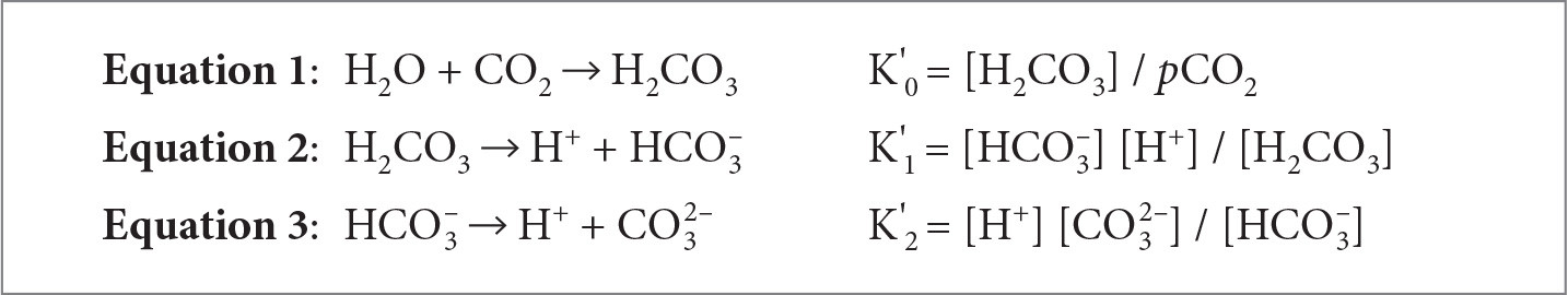
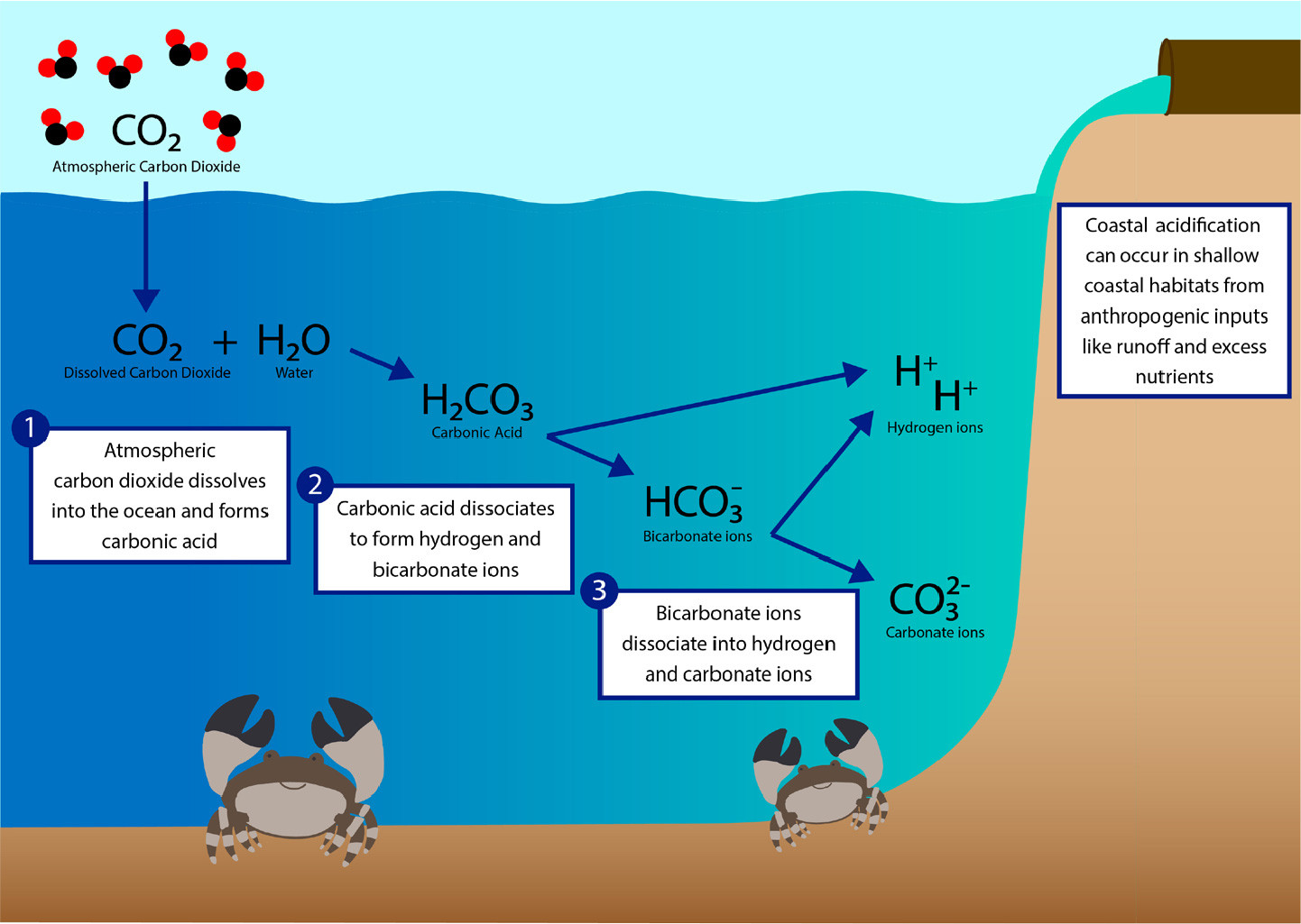
Since the Industrial Revolution, the release of fossil fuels in combination with other anthropogenic activities (i.e., coastal development, eutrophication, discussed below) have caused atmospheric carbon dioxide (CO₂) concentrations to increase (Tans, 2009). Oceanic surface waters have absorbed between 20% and 30% of the released atmospheric CO₂ since the 1980s, thus reducing seawater pH in a process called ocean acidification (Feely et al., 2009; IPCC, 2018). Ocean acidification occurs through a series of chemical reactions that results in the increase of the partial pressure of CO₂ in seawater (pCO₂), dissolved inorganic carbon (DIC), the concentration of H⁺ ions, and the concentration of bicarbonate ions (HCO₃^–). During this process the concentration of carbonate ions (CO₃^2–) and seawater pH both decrease, although the carbonate species favored as seawater pH decreases is bicarbonate (Feely et al., 2009). The dissolution of CO₂ into the ocean forms carbonic acid (H₂CO₃; Equation 1; Figure 1), which can easily dissociate in seawater to form hydrogen (H⁺) and bicarbonate ions (HCO₃^–; Equation 2; Figure 1). The HCO₃^– also dissociates, shifting the equilibrium constants to favor elevated CO₂ and more H⁺ ions (Equation 3; Figure 1). This series of reactions changes the buffering capacity of seawater, so that the seawater pH, measured as the concentration of H⁺ ions in a solution, is reduced, that is, it becomes less basic. Currently, the ocean’s pH is around 8.0–8.1, which is considered basic; however, as more CO₂ dissolves into the ocean, the pH will decrease, resulting in a less basic environment (i.e., pH < 8.0). The species in brackets in Equations 1–3 represent the equilibrium relationships among the species in the ocean acidification reactions (Dickson, 2011).

 

> High res equations

 

FIGURE 1. Sketch of the chemistry that underlies ocean acidification. pH is defined as the amount of H+ ions in a solution, so as the amount of H+ ions increases through these reactions, the pH decreases, making the seawater less basic. In shallow coastal habitats, pH can also be reduced by coastal inputs such as runoff and excess nutrient loads. Seasonal changes can also reduce coastal pH. Additional information on the chemical reactions can be found in Feely et al. (2009). Illustration by Samantha Stewart. > High res figure

 

Coastal Acidification

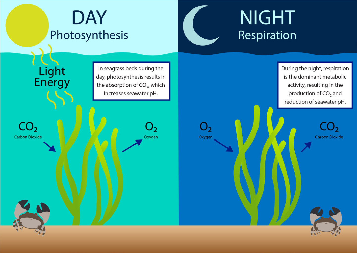
Both anthropogenic activities and natural phenomena can cause reductions in coastal seawater pH (Barton et al., 2015; Ekstrom et al., 2015). Shallow coastal habitats, which have smaller volumes of water relative to the open ocean, make these environments more susceptible to fluctuations in seawater pH (Millero et al., 2001; Yates et al., 2007; Manzello et al. 2012; Wallace et al., 2014; Enochs et al., 2019). Such changes can arise from a combination of processes such as the biological activity of benthic communities (diel changes from photosynthesis and respiration), storm events, and seasonal changes in carbonate chemistry (Millero et al., 2001; Yates et al., 2007; Manzello et al., 2012; Wallace et al., 2014; Barton et al., 2015; Enochs et al., 2019). These natural fluctuations in coastal pH can also be exacerbated by excess nutrient-​rich runoff and changes in land use (Gledhill et al., 2015). For example, the seepage of groundwater and upwelling events can elevate pCO₂ and thus reduce seawater pH in coastal areas (Basterretxea et al., 2010; Duarte et al., 2013; Breitburg et al., 2015; Gledhill et al., 2015). In addition, riverine input is acidic relative to coastal seawater, and the decomposition of the associated organic runoff (nitrogen and phosphorous) can contribute to reductions in coastal seawater pH (Duarte et al., 2013). Finally, coastal habitats (within 1 km from the coast) such as seagrass, mangroves, and coral reefs can be metabolically intense, resulting in diel changes in pH that can be as high as 1 pH unit (Brussaard et al., 1996; Spilling, 2007; Dai et al., 2008; Duarte et al., 2013; see Figure 2). Although metabolism plays a role in diel fluctuations in seawater pH within habitats like seagrass, it is important to note that pH can be affected hourly or seasonally by other biogeochemical and physical processes such as upwelling events, plankton blooms, and watershed inputs (Kapsenberg and Cyronak, 2019).

 

FIGURE 2. Depiction showing the diel changes that can occur from processes like photosynthesis and respiration in habitats like seagrass beds. During the day, photosynthetic activity can result in an increase in seawater pH. During the night, respiration becomes the dominant metabolic process resulting in a release of CO2, which then reduces seawater pH. Illustration by Samantha Stewart. > High res figure

 

Extreme changes in coastal pH may therefore have consequences for some coastal species, especially during embryonic, larval, and juvenile developmental stages, which are often more sensitive to environmental stressors than adult stages (Whiteley, 2011; Munday et al., 2012; Gledhill et al., 2015; Gravinese, 2018; Gravinese et al., 2018, 2019). Alternatively, prior exposure to fluctuating seawater pH may allow a species to acclimate so that individuals can tolerate extremes in seawater pH (Byrne, 2011; Thor and Dupont, 2017).

 

The Florida Stone Crab Fishery: A Case Study

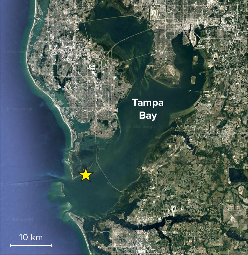
Shallow coastal habitats are important settlement and nursery grounds for many commercially significant species. One such fishery in Florida is the stone crab (Menippe mercenaria), which can be found in many coastal habitats ranging from North Carolina to the Florida peninsula (Muller et al., 2011). Stone crabs occupy shallow subtidal habitats to depths of 60 m (Lindberg and Marshall, 1984). In South Florida, the stone crab fishery is valued at $25–$30 million per year and occurs in a variety of coastal and nearshore habitats (e.g., muddy, shell fragment, and hard bottoms; rocky subtidal riprap; seagrass) along Florida’s Gulf Coast, including lower Tampa Bay (Figure 3; Muller et al., 2011; Bert et al., 2021). Stone crabs have been overfished since 2000, with mean annual landings declining by about 30% since that time (Muller et al., 2011).

 

FIGURE 3. Map of Tampa Bay, Florida. The yellow star indicates the study site used in Activity 4 described in the text. The image was taken from Google Earth, https://earth.google.​com/​web/​​@27.​76163495,​​-82.​57939235,​11.​66303789a,​106179.​01983803d,​35y,0h,0t,0r. > High res figure

 

Stone crabs are reproductive during the spring-summer seasons. Egg brooding, embryonic development, larval release, and settlement of juvenile stone crabs all occur in coastal, nearshore habitats (Lindberg and Marshall, 1984; Krimsky and Epifanio, 2008). After hatching, stone crab larvae are transported offshore to complete about a month of larval development before they return to shallow coastal habitats as juveniles (Gravinese et al., 2019). Reductions in seawater pH are threatening the stone crab fishery. In recent studies, stone crab embryos exhibited a 28% decrease in hatching success, while the larvae exhibited a 37% increase in mortality when maintained in low pH water (Gravinese, 2018; Gravinese et al., 2018). During exposure to present-day pH conditions (pH = 8.0) in a laboratory-​based experiment, the majority of larval stone crabs swam upward (~20%–50% swam down); however, stone crab larvae that were raised in seawater with reduced pH in the laboratory reversed their swimming direction, with more larvae swimming downward (~60%–100%) and at a faster rate than larvae raised in present-day pH experimental conditions (Gravinese et al., 2019). Combined, these studies suggest that changes in seawater pH may threaten the future sustainability of one of Florida’s most prized crustacean fisheries.

Comparisons among populations that naturally experience different levels of pH variability can serve as a “natural laboratory” for estimating the future reproductive success of a species to ocean acidification extremes (Thomsen et al., 2017). Identifying resilient sub-populations and potential refugia from ocean acidification is critical to preserving local habitats that provide ecosystem services such as those that contribute to the future sustainability of Tampa Bay’s local fisheries. Based on scientific research, we provide a suite of activities aimed at comparing the reproductive success and tolerance of Tampa Bay stone crabs whose habitats exhibit a range of pH values (e.g., seagrass vs. bare sandy substrates).

 

RESEARCH QUESTIONS AND HYPOTHESES

During this guided-inquiry exercise, students compare the variability in seawater pH in sand and seagrass habitats located within Tampa Bay, Florida, and determine how reductions in seawater pH may impact stone crab reproductive success. In Activity 1, students interact and analyze data from an online coastal acidification monitoring buoy in Tampa Bay to identify relationships among pH, pCO₂, and temperature. During Activity 2, students analyze subsets of experimental field chemistry data to develop hypotheses about how the pH will vary between seagrass (which has greater pH variability due to biological processes like photosynthesis and respiration) and sand habitats (which have lower pH variability due to a reduced level of photosynthesis relative to seagrass sites). Activities 3 and 4 then challenge students to make predictions about how exposure to variable seawater pH may impact stone crab reproductive success in a future, more acidic ocean and hypothesize how changes in seawater pH may affect the future stone crab fishery.

To ensure that students have a general understanding of the biology and ecology of stone crabs and ocean acidification, we encourage teachers to provide background information prior to completing the lesson through discussion or a student-​led, online scavenger hunt about ocean acidification concepts (e.g., https://www.​pmel.​noaa.​gov/​co2/​story/​What+​is+​Ocean+​Acidification%3F). If time permits, we encourage instructors to supplement this lesson with other hands-on activities published in Oceanography that focus on ocean acidification concepts (see Boleman et al., 2013; Murphy and Measures, 2014). We also recommend that educators explore pH-specific concepts with students prior to this lesson (e.g., https://www.​pmel.​noaa.​gov/​co2/​story/​A+​primer+​on+​pH). We provide a glossary of terms that students can reference throughout the lesson (see the online Supplementary Materials).

 

Activity 1: Monitoring Variability in Seawater pH in Tampa Bay, Florida

Time: 40–60 minutes, one class period or homework assignment

Activity 1 challenges students to characterize the relationships among pH, pCO₂, and temperature using data from the US Geological Survey’s open-access online monitoring system in Tampa Bay (http://tampabay.loboviz.com/). During this activity, students explore the Tampa Bay Land/Ocean Biological Observatory (LOBO) website and plot the environmental data provided by the buoy to make comparisons relative to the pH conditions within Tampa Bay to help them identify how these variables are related. After plotting the data, students answer the questions provided.

 

Activity 1 Materials

• Computer with internet access

 

Activity 1 Directions for Students

1. Access the Tampa Bay LOBO website (http://tampabay.loboviz.com/). Look over the information on the home tab to learn about the observatory.

2. Go to the “LOBOVIZ” tab. To evaluate the pH, pCO₂, and temperature within Tampa Bay during summer 2021, you will need to access data collected by the observatory. To create plots and analyze relationships, select CO₂ for the “X Variable” and pH for the “Y Variable.” Select and specify the “Date Range” Start and End dates. Specify the start as 2021 July 01 and the end as 2021 July 31. Click “Plot the Data” to create the plot. Observe the trend between pCO₂ and pH.

3. Repeat the previous step, but with temperature on the x-axis. Observe the trend between temperature and pH.

4. Using the plots created via the Tampa Bay LOBO website, answer the extension questions.

Note: If students are unable to access the Tampa Bay LOBO website, we provide an Excel file of data and a handout with directions for plotting the data in the online Supplementary Materials.

 

Activity 1 Discussion Questions

The instructor can use the following questions to foster a class discussion that helps highlight how pH, pCO₂, and temperature are related in Tampa Bay during the sampling time specified.

1. Explain the relationship between pH and pCO₂. Use the plot you created as evidence.

2. Explain the relationship between pH and temperature. Use the plot you created as evidence.

3. What other environmental variables do you hypothesize may influence sea­water pH? Explain your reasoning for this prediction.

 

Activity 2: Do seagrass habitats have more variable pH conditions than sandy habitats in Tampa Bay?

Time: 40–60 minutes, one class period or homework assignment

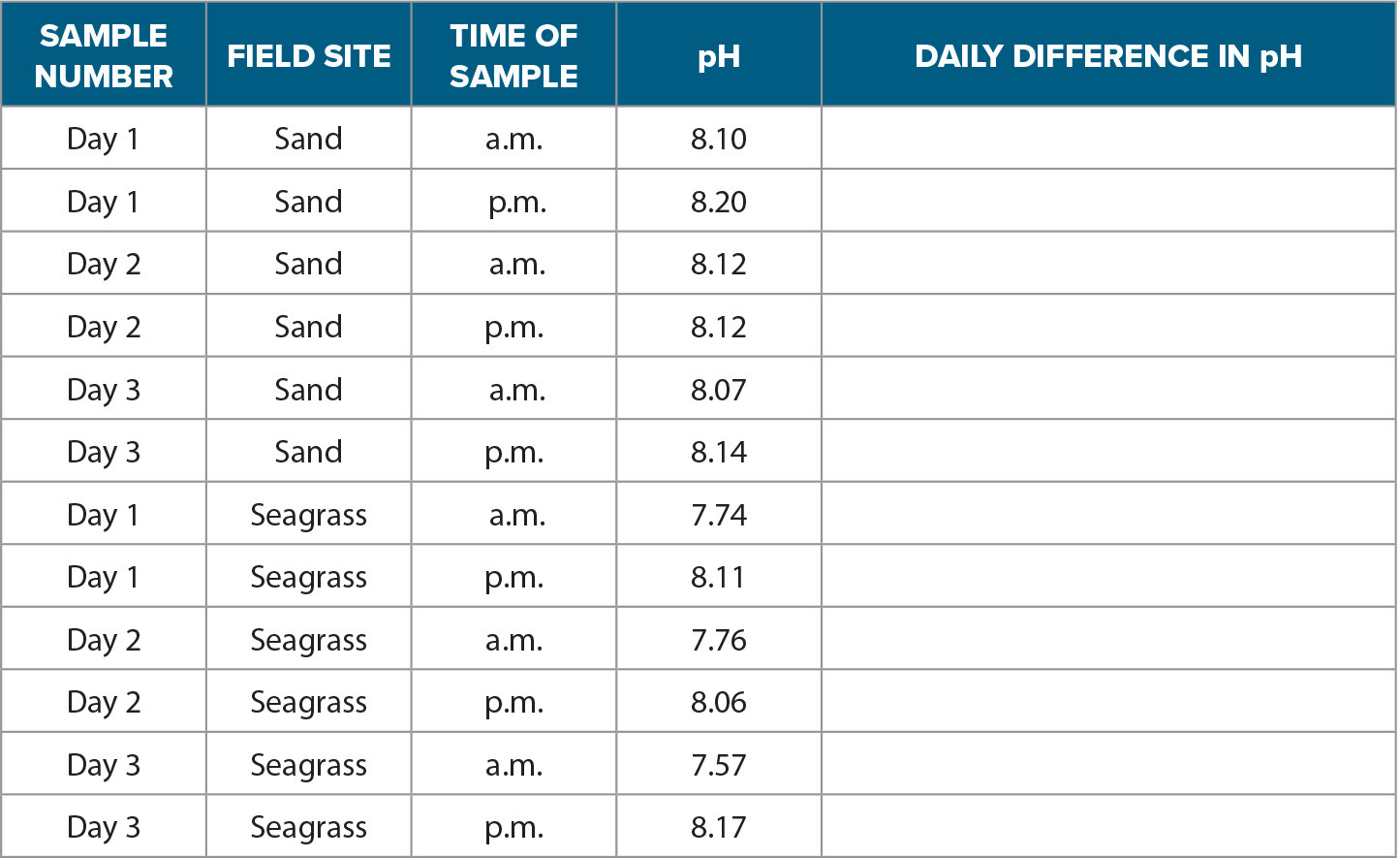
Activity 2 characterizes the diel relationships in seawater pH between seagrass and sand habitats using data collected during an experiment conducted in Tampa Bay. Students begin Activity 2 by plotting seawater pH during sunrise and sunset from both research sites (Table 1). After plotting the data, students then calculate the daily variability of pH by subtracting the maximum and minimum values for each day at the sand site and at the seagrass site to determine the differences in pH variability. Finally, students answer the questions provided.

 

TABLE 1. A subset of the daily (a.m. and p.m.) pH (error ±0.01) at each field site (sand and seagrass) measured during the study. The pH values have been rounded to the hundreds place to represent better accuracy for this activity, though most pH measurements in ocean acidification studies are to the thousands decimal place. Students can use the last column of this table to calculate the daily variability for each site by subtracting the daily minimum from the daily maximum pH value. > High res table

 

Activity 2 Materials

• Data table with the pH data from the seagrass and sand research sites within Tampa Bay from the 2020–2021 study

• Calculator

• Computer with graphing software (e.g., Excel, Google Sheets)

 

Activity 2 Directions for Students

1. Use the data table provided to create a line plot in Excel or Google Sheets to depict the variability of seawater pH for the seagrass and sand field sites. The pH should be plotted on the y-axis. The x-axis will be the time of the sample. The plot should have two lines, one for the sand site and one for the seagrass site. Be sure to label the units where appropriate.

2. After creating the plot, calculate the daily variability by subtracting the minimum pH value from the maximum pH value for each day in the seagrass site and each day in the sand site.

3. Using the line plot and the calculated daily variability, answer the Activity 2 discussion questions.

 

Activity 2 Discussion Questions

The instructor can use the following questions and directions to foster a class discussion that will help highlight how biological processes within different habitats, like seagrass and sand, may impact coastal pH. This time can be used to introduce the relationship between pH and pCO₂.

1. Explain how pH changed within each field site. Use the calculations and plot you created as evidence.

2. Explain the relationship between pH and photosynthesis and respiration. Use the plot you created as evidence.

3. Warmer water holds less CO₂ than colder water, but the results in Activity 1 from the data buoy show the opposite trend. Explain why this might be happening.

4. Hypothesize how pH might impact the reproductive success of stone crabs; use the plot and prior knowledge to formulate a hypothesis.

 

Activity 3: Does reduced seawater pH change stone crab hatching success?

Time: 30–40 minutes

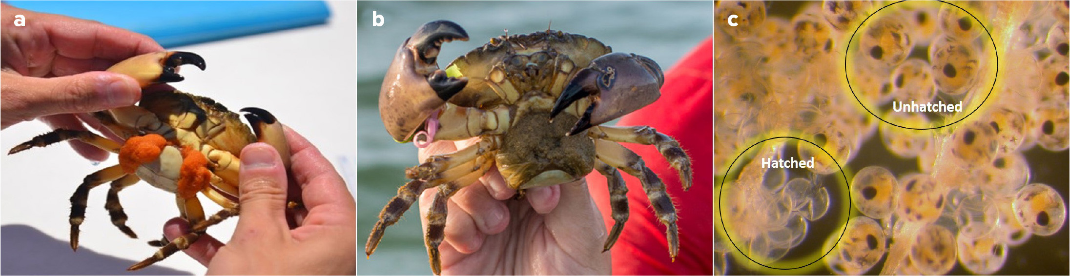
Activity 3 is modeled after an experiment that was designed to determine the reproductive success of stone crabs under static pH conditions. It included an ambient, present-day pH condition (pH = 8.0) vs. a more acidic end-of-century pH condition (pH = 7.6; see Gravinese, 2018). During this experiment, stone crabs with early stage embryos (orange in Figure 4a) were collected and brought back to Mote Marine Laboratory and Aquarium, acclimated over 24 hours, and then randomly placed within the two different pH treatments. Only crabs with early stage embryos (i.e., an orange stage egg mass) were used. The crab eggs were checked daily for embryo development by taking images using a digital microscope. This allowed scientists to identify when the embryos were within 24 hrs of hatching (brown egg mass in Figure 4b). At that time, a cluster of embryos (~100) was removed from the egg mass and placed in a separate container with the same pH conditions as the brooding female. After the female crab completed hatching, hatching success was determined by counting the number that hatched vs. the number that did not hatch in the sample of removed embryos for control and reduced pH treatments (Figure 4c). Embryos in the control had 76% hatching success, while embryos in the reduced pH treatment had 48% hatching success.

 

FIGURE 4. Photos of (a) an ovigerous stone crab with early stage developed (orange) embryos, and (b) an ovigerous stone crab with late stage developed embryos (brown). (c) A microscope image shows stone crab embryos that are hatched (clear embryos) vs. embryos that are unhatched (embryo presents with large eyespot). Image credit: Philip Gravinese and Florida Southern College. > High res figure

 

The physiological mechanisms responsible for the reduction in hatching success were not identified in the study described above; however, the authors provide some explanation based on the results of similar studies conducted on crustaceans. The reduction in hatching success in the study described was likely the result of embryos undergoing acidosis, or the acidification of the body fluids, which could potentially damage cardiac cells within the embryo (Ceballos-Osuna et al., 2013). Damage to cardiac tissues could result in lower oxygen availability or reduce the amount of CO₂ removed, which could limit metabolic output (Ceballos-Osuna et al., 2013). Alternatively, because crab embryos require more oxygen as they get closer to hatching, later stage embryos may have difficulty exchanging O₂ or CO₂ gases, and reduced pH could limit hatching (Naylor et al., 1999; Brante et al., 2003).

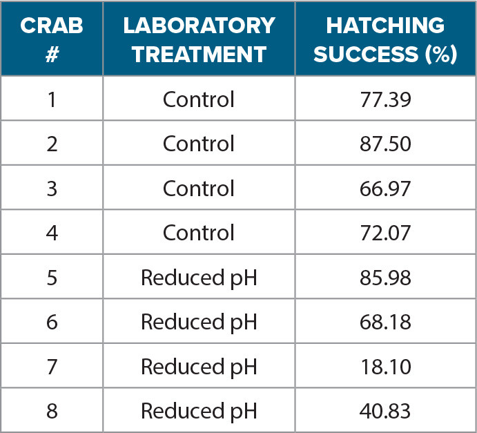
There was also greater variability in the number of embryos that hatched during the reduced pH treatment, which ranged from 18% to 85%, while hatching success in the control ranged from 66% to 87%. The researchers hypothesized that this variability in hatching success may be related to the environmental history of the female crab during embryogenesis (see Activity 4) and could represent potential for adaptation.

During Activity 3, students determine the effect of reduced seawater pH on stone crab reproduction by plotting and comparing trends in hatching success between the two treatments (control vs. reduced pH; Table 2). After plotting the data, students answer the questions provided for Activity 3. The data used in this activity is only a subset of the data collected by the scientists during this work. We want to stress to both the educators and students that experiments such as the ones presented in this lesson often require a much larger sample size.

 

TABLE 2. A subset of hatching success (%) data from eight different stone crabs that were exposed to either the control (n = 4) or reduced pH (n = 4) treatments. > High res table

 

Activity 3 Materials

• Data table with the hatching success data from the 2018 study

• Calculator

• Computer with graphing software (e.g., Excel, Google Sheets)

 

Activity 3 Directions for Students

1. Use the data table provided to calculate the average hatching success for the control and reduced pH treatments using Excel or Google Sheets. The average can be calculated by summing the data points in the sample and then dividing that sum by the sample size (total number of data points collected). To calculate the average in Excel, use the built-in average function by typing the following code into a cell: “=AVERAGE(cells).” After typing this code, you will then be able to select the data (cells) for the calculation.

2. Next, calculate the standard deviation and standard error for each treatment in Excel or Google Sheets. The formula for calculating a standard deviation (σ) is:

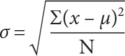Where x is a collected data point, µ is the population mean, and N is the sample size. To calculate standard deviation in Excel, use the code: =STDEVA(cells). After typing this code, select the data (cells) for the calculation.

The formula for calculating standard error is:

where σ is the standard deviation and N is the sample size. To calculate standard error in Excel, use the code: =STDEVA(cells)/SQRT(COUNT(cells)). After typing this code, select the data (cells) for the calculation.

3. Use the calculated average hatching success to create a bar graph with standard error bars, using Excel or Google Sheets, that compares the average hatching success for each treatment. Be sure to label the axis and include units where appropriate in Excel. To add custom standard error bars in Excel, access the “Format Error Bars” window. In the error bar option tab, under “Error Amount” select “Custom” and specify value as the calculated standard error values for both the positive and negative error values.

4. Using the bar graph, answer the Activity 3 discussion questions.

 

Activity 3 Discussion Questions

The instructor can use the following questions to foster discussions that will help highlight the impact of reduced pH on stone crab reproduction.

1. What can cause reduced seawater pH? List one natural and one anthropogenic cause.

2. Which treatment had a higher hatching success? Use the averages and plot as evidence.

3. Discuss which treatment might lead to lower reproductive success for the population. Use the averages, plots, and prior knowledge to formulate your hypothesis.

4. If the average legal-sized female stone crab of 102 mm in carapace width has an annual fecundity around 2 million eggs (Ros et al., 1981; Hogan and Griffen, 2014), use the average hatching success from this study to estimate how the reduction in hatching success in reduced pH seawater may affect the fecundity of a single crab in one reproductive season (one year).

 

Activity 4: Does prior exposure to variable pH conditions result in better hatching success in stone crabs?

Time: 30–45 minutes

In Activity 4, students analyze a subset of the data provided from a recent experiment designed to determine whether exposure to more variable pH habitats affects stone crab reproductive success. They use the data provided in Table 3 to calculate the average hatching success of crabs conditioned in the two different field locations: seagrass and sand. After plotting the data, students answer the questions for Activity 4.

 

TABLE 3. A subset of the hatching success (%) experimental data from 12 different stone crabs that were conditioned in either seagrass or sandy habitats prior to forming a new egg mass. Once a new egg mass was formed, the crabs were then transported and placed in an ocean acidification experimental system that mimicked the 2018 study. The crabs in the experimental system were assigned to either a reduced pH (7.7) or control treatment pH (8.0). > High res table

 

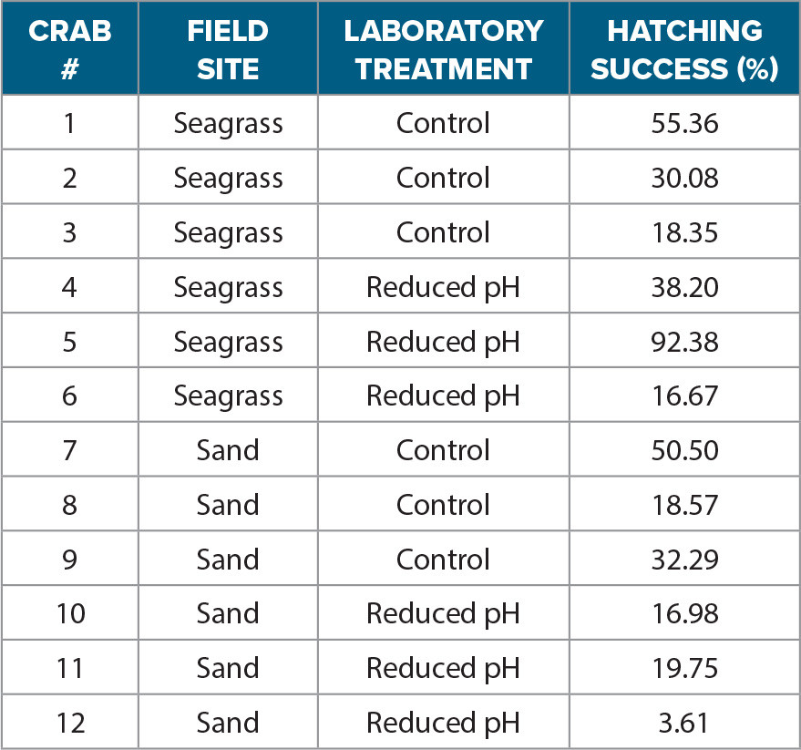
The goal of the experiment used for this activity was to determine if more variable pH habitats (i.e., seagrass) had any effect on the reproductive success of stone crabs. Egg-bearing stone crabs were collected and conditioned in either a sandy habitat with a narrow daily range of pH (7.9–8.1) or in a seagrass habitat with a greater daily range of pH (7.7–8.1). The crabs in both habitats were fed and monitored every other day until they released their current egg mass and then developed a new egg mass within each respective habitat. Crabs that developed a new egg mass (>7 days conditioning in their field site) were then transported back to an ocean acidification laboratory at Florida Southern College and randomly assigned to either a control pH (8.0) or a reduced pH (7.7) treatment for the duration of their embryo development period. Crabs were acclimated to laboratory conditions for 24 hrs. Each crab’s hatching success was monitored in both treatments similar to the description in Activity 2. Hatching success (%) was then calculated for each crab in each treatment (Table 3).

 

Activity 4 Materials

• Data table with the hatching success data from the 2020–2021 study

• Calculator

• Computer with graphing software (e.g., Excel, Google Sheets)

 

Activity 4 Directions for Students

1. Use the data table provided to calculate the average hatching success for the control and reduced pH treatments from each field site using Excel or Google Sheets. Calculate four averages by summing the data points in the sample and then dividing that sum by the sample size (total number of data points collected). To calculate the average in Excel, use the built-​in average function described in the previous activity.

2. Next, calculate the standard deviation and standard error for each treatment using Excel or Google Sheets. The formula for calculating a standard deviation (σ) and standard error were described in the previous activity.

3. Use the calculated average hatching success to create a bar graph with standard error bars in Excel or Google Sheets that compares the average hatching success for each treatment. Be sure to label the axis and include units where appropriate. Use the custom standard error bars described for Excel in the previous activity’s directions.

4. Using the bar graph, answer the Activity 4 discussion questions.

 

Activity 4 Discussion Questions

The instructor can use the following questions to foster discussions that will help highlight the impact of more variable pH in both sand and seagrass environments on stone crab reproduction.

1. Which treatment and habitat had a higher hatching success? Use the averages and plot as evidence.

2. Discuss which treatment and habitat might lead to higher reproductive success for stone crabs. Use the averages, plots, and prior knowledge to formulate a hypothesis.

3. Is there any variation in the hatching success results observed in crabs from the sand and seagrass habitats? If so, what could be the reason for these differences?

4. Predict what these results may indicate for the stone crab fishery under future climate conditions.

5. Based on these results, what management actions would you recommend in order to mitigate the impacts of climate change on stone crabs?

 

ACKNOWLEDGMENTS

We thank the Florida Fish and Wildlife stone crab independent monitoring program for assistance with animal collection. Stone crabs were collected under a Florida Fish and Wildlife Special Activity License (#SAL-20-1868B-SR). The subsets of data presented in these activities were supported by a Mote Marine Laboratory and Aquarium Protect Our Reef License Plate grant (POR-2011-27) and a Tampa Bay Environmental Restoration Fund grant. Gravinese’s current research is supported by a National Science Foundation grant OCE-2049047. We also acknowl­edge K. Yates and C. Moore from the US Geological Survey in St. Petersburg for analysis of seawater car­bonate chemistry samples and who curate the Land/Ocean Biogeochemical Observatory (LOBO). The buoy is curated in collaboration with the Ocean Carbon System (OCS) at the USF Center for Maritime and Port Studies and the Tampa Bay Physical Oceanographic Real Time System (http://tbports.org/) to provide real-time, high-resolution water quality data through this interactive website. All data from the website are provisional pending USGS approval.

Gravinese, P.M., A.L. Smith, S.M. Stewart, and J. Paradis. 2023. Do pH-variable habitats provide refuge for stone crabs from coastal acidification? Oceanography 36(1):59–66, https://doi.org/10.5670/oceanog.2023.105.

• Glossary of Terms
• Lesson Answer Key
• List of Additional Resources
• Activity 1 Handout and Table S1 (Excel data file) — for use if students cannot access the Tampa Bay LOBO website

Barton, A., G.G. Waldbusser, R.A. Feely, S.B. Weisberg, J.A. Newton, B. Hales, S. Cudd, B. Eudeline, C.J. Langdon, I. Jefferds, and others. 2015. Impacts of coastal acidification on the Pacific Northwest shellfish industry and adaptation strategies implemented in response. Oceanography 28(2):146–149, https://doi.org/10.5670/oceanog.2015.38.

Basterretxea, G., A. Tovar-Sanchez, A.J. Beck, P. Masqué, H.J. Bokuniewicz, R. Coffey, C.M. Duarte, J. Garcia-Orellana, E. Garcia-Solsona, L. Martinez-Ribes, and R. Vaquer-Sunyer. 2010. Submarine groundwater discharge to the coastal environment of a Mediterranean island (Majorca, Spain): Ecosystem and biogeochemical significance. Ecosystems 13:629–643, https://doi.org/​10.1007/s10021-010-9334-5.

Bert, T.M., C. Crawford, and C. Shea. 2021. Young-of-the-year stone crab (Genus Menippe) recruitment in the Gulf of Mexico off Florida: Key shallow-water hotspots. Journal of Shellfish Research 40(2):339–398, https://doi.org/​10.2983/​035.040.0211.

Boleman, C.L., P.M. Gravinese, E.N. Muse, A.E. Marston, and J.G. Windsor. 2013. Corals on acid: An inquiry-based activity leading students to a better understanding of ocean acidification impacts. Oceanography 26(4):164–169, https://doi.org/​10.5670/oceanog.2013.87.

Brante, A., M. Fernández, L. Eckerle, F.C. Mark, H.O. Pörtner, and W. Arntz. 2003. Reproductive investment in the crab Cancer setosus along a latitudinal cline: Egg production, embryo losses and embryo ventilation. Marine Ecology Progress Series 251:221–232, https://doi.org/10.3354/meps251221.

Breitburg, D.L., J. Salisbury, J.M. Bernhard, W.-J. Cai, S. Dupont, S.C. Doney, K.J. Kroeker, L.A. Levin, W.C. Long, L.M. Milke, and others. 2015. And on top of all that… Coping with ocean acidification in the midst of many stressors. Oceanography 28(2):48–61, https://doi.org/​10.5670/oceanog.2015.31.

Brussaard, C.P.D., G.J. Gast, F.C. van Duyl, and R. Riegman. 1996. Impact of phytoplankton bloom magnitude on a pelagic microbial food web. Marine Ecology Progress Series 144:211–221, https://doi.org/​10.3354/meps144211.

Byrne, M. 2011. Impact of ocean warming and ocean acidification on marine invertebrate life history stages. Chapter in Oceanography and Marine Biology. CRC Press.

Ceballos-Osuna, L., H.A. Carter, N.A., Miller, and J.H. Stillman. 2013. Effects of ocean acidification on early life-history stages of the intertidal porcelain crab Petrolisthes cinctipes. Journal of Experimental Biology 216:1,405–1,411, https://doi.org/10.1242/jeb.078154.

Dai, M., W. Zhai, W. Cai, J. Callahan, B. Huang, S. Shang, T. Huang, X. Li, Z. Lu, and W. Chen. 2008. Effects of an estuarine plume-associated bloom on the carbonate system in the lower reaches of the Pearl River estuary and the coastal zone of the northern South China Sea. Continental Shelf Research 28:1,416–1,423, https://doi.org/10.1016/​j.csr.2007.04.018.

Dickson, A.G. 2011. The carbon dioxide system in seawater: Equilibrium chemistry and measurements. Pp 17–40 in Guide to Best Practices for Ocean Acidification Research and Data Reporting. U. Riebesell, V.J. Farby, L. Hanson, and J.P. Gattuso, eds, European Commission, Brussels.

Duarte, C.M., I.E. Hendriks, T.S. Moore, Y.S. Olsen, A. Steckbauer, L. Ramajo, J. Carstensen, J.A. Trotter, and M. McCulloch. 2013. Is ocean acidification an open-ocean syndrome? Understanding anthropogenic impacts on seawater pH. Estuaries and Coasts 36(2):221–236, https://doi.org/10.1007/s12237-013-9594-3.

Ekstrom, J.A., L. Suatoni, S.R. Cooley, L.H. Pendleton, G.G. Waldbusser, J.E. Cinner, J. Ritter, C. Langdon, R. Van Hooidonk, D. Gledhill, and K. Wellman. 2015. Vulnerability and adaptation of US shellfisheries to ocean acidification. Nature Climate Change 5(3):207–214, https://doi.org/10.1038/nclimate2508.

Enochs, I.C., D.P. Manzello, P.R. Jones, S.J. Stamates, and T.P. Carsey. 2019. Seasonal carbonate chemistry dynamics on southeast Florida coral reefs: Localized acidification hotspots from navigational inlets. Frontiers in Marine Science 6, 160, https://doi.org/​10.3389/fmars.2019.00160.

Feely, R.A., S.C. Doney, and S.R. Cooley. 2009. Ocean acidification: Present conditions and future changes in a high-CO₂ world. Oceanography 22(4):36–47, https://doi.org/​10.5670/oceanog.2009.95.

Gledhill, D.K., M.M. White, J. Salisbury, H. Thomas, I. Mlsna, M. Liebman, B. Mook, J. Grear, A.C. Candelmo, R.C. Chambers, and others. 2015. Ocean and coastal acidification off New England and Nova Scotia. Oceanography 28(2):182–197, https://doi.org/10.5670/oceanog.2015.41.

Gravinese, P.M. 2018. Ocean acidification impacts the embryonic development and hatching success of the Florida stone crab, Menippe mercenaria. Journal of Experimental Marine Biology and Ecology 500:140–146, https://doi.org/10.1016/​j.jembe.2017.09.001.

Gravinese, P.M., I.C. Enochs D.P. Manzello, and R. van Woesik. 2018. Warming and pCO₂ effects on Florida stone crab larvae. Estuarine, Coastal and Shelf Science 204:193–201, https://doi.org/10.1016/​j.ecss.2018.02.021.

Gravinese, P.M., I.C. Enochs, D.P. Manzello, and R. van Woesik. 2019. Ocean acidification changes the vertical movement of stone crab larvae. Biology Letters 15(12), 20190414, https://doi.org/10.1098/rsbl.2019.0414.

Hogan, J.M., and B.D. Griffen. 2014. The dietary and reproductive consequences of fishery-related claw removal for the stone crab Menippe spp. Journal of Shellfish Research 33(3):795–804, https://doi.org/​10.2983/035.033.0314.

IPCC. 2018. Global Warming of 1.5°C. An IPCC Special Report on the Impacts of Global Warming of 1.5°C Above Pre-Industrial Levels and Related Global Greenhouse Gas Emission Pathways, in the Context of Strengthening the Global Response to the Threat of Climate Change, Sustainable Development, and Efforts to Eradicate Poverty. V. Masson-Delmotte, P. Zhai, H.-O. Pörtner, D. Roberts, J. Skea, P.R. Shukla, A. Pirani, W. Moufouma-Okia, C. Péan, R. Pidcock, and others, eds, Cambridge University Press, Cambridge, UK, and New York, NY, USA, 616 pp.

Kapsenberg, L., and T. Cyronak. 2019. Ocean acidification refugia in variable environments. Global Change Biology 25(10):3,201–3,214, https://doi.org/​10.1111/gcb.14730.

Kealoha, A.K., K.E. Shamberger, S.F. DiMarco, K.M. Thyng, R.D. Hetland, D.P. Manzello, N.C. Slowey, and I.C. Enochs. 2020. Surface water CO₂ variability in the Gulf of Mexico (1996–2017). Scientific Reports 10(1), 12279, https://doi.org/​10.1038/​s41598-020-68924-0.

Krimsky, L.S., and C.E. Epifanio. 2008. Multiple cues from multiple habitats: Effects on metamorphosis of the Florida stone crab, Menippe mercenaria. Journal of Experimental Marine Biology and Ecology 358:178–184, https://doi.org/10.1016/​j.jembe.2008.02.010.

Lindberg, W.J., and M.J. Marshall. 1984. Species Profiles: Life Histories and Environmental Requirements of Coastal Fishes and Invertebrates (South Florida)—Stone Crab. US Fish Wildlife Service, FWS/OBS-82/11.21, US Army Corps of Engineers, TR EL-82-4,17 pp.

Lohrenz, S.E., W.J. Cai, S. Chakraborty, W.J. Huang, X. Guo, R. He, Z. Xue, K. Fennel, S. Howden, and H. Tian. 2018. Satellite estimation of coastal pCO₂ and air-sea flux of carbon dioxide in the northern Gulf of Mexico. Remote Sensing of Environment 207:71–83, https://doi.org/10.1016/​j.rse.2017.12.039.

Manzello, D.P., I.C. Enochs, N. Melo, D.K. Gledhill, and E.M. Johns. 2012. Ocean acidification refugia of the Florida Reef Tract. PLoS ONE 7(7), 41715, https://doi.org/​10.1371/journal.pone.0041715.

McCutcheon, M.R., H. Yao, C.J. Staryk, and X. Hu. 2021. Temporal variability and driving factors of the carbonate system in the Aransas Ship Channel, TX, USA: A time series study. Biogeosciences 18(15):4,571–4,586, https://doi.org/​10.5194/bg-18-4571-2021.

Millero, F.J., W.T. Hiscock, F. Huang, M. Roche, and J.Z. Zhang. 2001. Seasonal variation of the carbonate system in Florida Bay. Bulletin of Marine Science 68(1):101–123.

Muller, R.G., D. Chagaris, T.M. Bert, C. Crawford, and R. Gandy. 2011. The 2011 Stock Assessment Update for the Stone Crab, Menippe spp., Fishery in Florida. Florida Fish and Wildlife Conservation Commission, St. Petersburg, FL, 55 pp.

Munday, P.L., M.I. McCormick, and G.E. Nilsson. 2012. Impact of global warming and rising CO₂ levels on coral reef fishes: What hope for the future? Journal of Experimental Biology 215:3,865–3,873, https://doi.org/10.1242/jeb.074765.

Murphy, J.L., and C.I. Measures. 2014. Ocean acidification: The role of CO₂. Oceanography 27(1):238–246, https://doi.org/​10.5670/​oceanog.2014.01.

Naylor, J., E. Taylor, and D. Bennett. 1999. Oxygen uptake of developing eggs of Cancer pagurus (Crustacea: Decapoda: Cancridae) and consequent behaviour of the ovigerous females. Journal of the Marine Biological Association of the United Kingdom 79(2):305–315, https://doi.org/10.1017/S0025315498000332.

Osborne, E., X. Hu, E.R. Hall, K. Yates, J. Vreeland-Dawson, K. Shamberger, L. Barbero, J.M. Hernandez-Ayon, F.A. Gomez, T. Hicks, and Y.Y. Xu. 2022. Ocean acidification in the Gulf of Mexico: Drivers, impacts, and unknowns. Progress in Oceanography, https://doi.org/10.1016/​j.pocean.2022.102882

Ros, R.M., D. Perez, and R. Rojas Manocal. 1981. Fecundidad en el cangrejo moro Menippe mercenaria. (Say, 1818) [Fecundity in the Stone crab Menippe mercenaria]. Revisita de Investigaciones Marinas 2:73–91.

Spilling, K. 2007. Dense sub-ice bloom of dinoflagellates in the Baltic Sea, potentially limited by high pH. Journal of Plankton Research 29: 895–901, https://doi.org/10.1093/plankt/fbm067.

Tans, P. 2009. An accounting of the observed increase in oceanic and atmospheric CO₂ and an outlook for the future. Oceanography 22(4):36–47, https://doi.org/10.5670/oceanog.2009.94.

Thomsen, J., L.A. Stapp, K. Haynert, H. Schade, M. Danelli, G. Lannig, K.M. Wegner, and F. Melzner. 2017. Naturally acidified habitat selects for ocean acidification-tolerant mussels. Science Advances 3(4), e1602411, https://doi.org/10.1126/sciadv.1602411.

Thor, P., and S. Dupont. 2015. Transgenerational effects alleviate severe fecundity loss during ocean acidification in a ubiquitous planktonic copepod. Global Change Biology 21:2,261–2,271, https://doi.org/​10.1111/gcb.12815.

Wallace, R.B., H. Baumann, J.S. Grear, R.C. Aller, and C.J. Gobler. 2014. Coastal ocean acidification: The other eutrophication problem. Estuarine, Coastal and Shelf Science 148:1–13, https://doi.org/10.1016/​j.ecss.2014.05.027.

Whiteley, N.M. 2011. Physiological and ecological responses of crustaceans to ocean acidification. Marine Ecology Progress Series 430:257–271, https://doi.org/10.3354/meps09185.

Yates, K.K., C. Dufore, N. Smiley, C. Jackson, and R.B. Halley. 2007. Diurnal variation of oxygen and carbonate system parameters in Tampa Bay and Florida Bay. Marine Chemistry 104(1–2):110–124, https://doi.org/10.1016/j.marchem.2006.12.008.

This is an open access article made available under the terms of the Creative Commons Attribution 4.0 International License (https://creativecommons.org/licenses/by/4.0/), which permits use, sharing, adaptation, distribution, and reproduction in any medium or format as long as users cite the materials appropriately, provide a link to the Creative Commons license, and indicate the changes that were made to the original content. Images, animations, videos, or other third-party material used in articles are included in the Creative Commons license unless indicated otherwise in a credit line to the material. If the material is not included in the article’s Creative Commons license, users will need to obtain permission directly from the license holder to reproduce the material.