PURPOSE OF ACTIVITY

This lesson uses data based on real-world geological archives to guide students toward understanding how climate and oceanographic conditions have impacted coral reef growth over the last 5,000 years. The objective of the lesson is for students to determine the relationship between environmental variability and coral reef development over millennial timescales. In this activity, students will:

1. Characterize the species composition and condition of coral reefs from different time periods in the past using cores that reveal reef architecture

2. Calculate the rate of calcium carbonate accretion (production) of the reefs during those past time intervals

3. Reconstruct trends in past climatic conditions using a mock data set

 

AUDIENCE

This lesson is designed for junior and senior high school students, as well as undergraduates in lower-level biology, marine biology, environmental chemistry, and oceanography courses. The activities will introduce students to paleoecological relationships associated with chemical variations in the coral skeleton, so the lessons may also be appropriate for courses in the geosciences. A glossary of terms for educators and students is provided in the online Notes for the Instructor and student Handout S1.

 

BACKGROUND

Coral reefs are among the most diverse ecosystems in the world, providing valuable ecosystem services to coastal communities by protecting them against wave energy and by contributing income from tourism and fishing to local economies (Moberg and Folke, 1999; Williams et al., 1999; Costanza et al., 2014). Coral reefs are found in tropical and subtropical areas where water temperatures are generally warm and stable. However, the growth of coral reefs and the ecosystem services they provide are threatened by thermal extremes (Hoegh-Guldberg et al., 2007; Manzello et al., 2008). Seawater temperatures are warming at most reef locations, increasing the frequency of coral bleaching (Hughes et al., 2018). Corals bleach following prolonged exposure to stressors, especially warming (thermal stress) combined with high light intensity. Coral bleaching involves the breakdown of the symbiotic relationship between corals and the single-​​celled dinoflagellate algae that live within their tissues. Corals rely on carbohydrates produced from photosynthesis by their symbiotic algae for 90% or more of their energetic needs, meaning that prolonged bleaching can be lethal (Glynn, 1993; Aronson et al., 2000; Lesser and Farrell, 2004; Anthony et al., 2007). Anomalously cold seawater temperatures can also cause bleaching and mortality, a problem for corals living in marginal environments such as zones where cold water upwells from the deeper ocean or regions such as Florida that are at the higher-latitude limits for warm-water coral growth (Roberts et al., 1982; Lirman et al., 2011; Wyatt et al., 2019).

 

Drivers of Coral Reef Growth: Oceanographic Variability in the Eastern Tropical Pacific

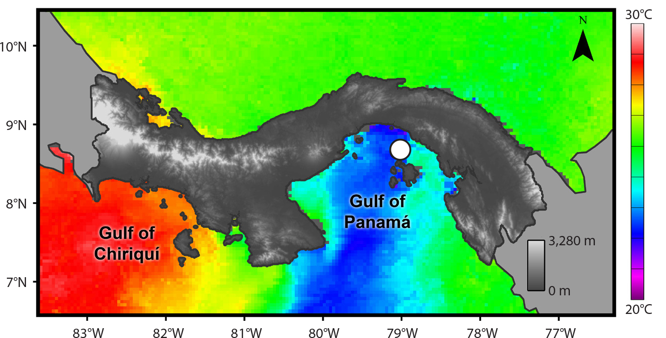
Environmental variability influences the growth of reef frameworks built by living corals over longer timescales. The oceanographic conditions in the eastern tropical Pacific (ETP) provide a natural laboratory for studying how environmental variability impacts the development of coral reefs over ecological and geological timescales. On an interannual scale, upwelling impacts reefs in many parts of the ETP, including Pacific Panamá (Randall et al., 2020; Figure 1). Upwelling in Pacific Panamá occurs during the boreal winter (December to April), when strong winds push surface waters offshore, allowing cold bottom waters that are rich in nutrients to flow toward the surface and exert a cooling influence on shallow-water environments. Temperature variability in Pacific Panamá is also influenced over interannual timescales by the phenomenon called the El Niño-Southern Oscillation (ENSO), which is the most significant control on reef development in the region. During an “ENSO-neutral” year, the trade winds blowing from east to west confine warmer sea surface waters to the western Pacific. During an El Niño year, the trade winds weaken, suppressing seasonal upwelling in the ETP. Alternatively, a La Niña year causes below-average, cooler sea surface temperatures in Pacific Panamá because stronger trade winds enhance seasonal upwelling (see https://oceanservice.noaa.gov/facts/ninonina.html for a visualization of ENSO). Scientists have hypothesized that coral reef health and growth in the ETP are driven by both seasonal upwelling and ENSO variability (Glynn, 1977; Glynn et al., 1992; Toth et al., 2012, 2017; Randall et al., 2020). Coral reefs located in the Gulf of Panamá have historically experienced strong seasonal upwelling, exposing them to cooler, more nutrient-rich, more turbid seawater conditions for three to four months each year, compared with nearby areas such as the Gulf of Chiriquí, where upwelling is weaker (Figure 1). The cooler water temperatures, elevated nutrients, and reduced pH levels that accompany seasonal upwelling are known to reduce coral growth (Glynn, 1977).

 

Figure 1. Map showing the study location (white dot) in the Gulf of Panamá in relation to the regional upwelling regimes. The ocean’s coloration depicts sea surface temperatures (SSTs) during the peak upwelling season in March 2009. The SST map was created using MODIS Aqua/SST data retrieved from NASA. Gray scale on the Isthmus indicates elevation obtained from http://srtm.csi.cgiar.org/. > High res figure

 

Geological Records Provide a Glimpse into Reefs’ Past

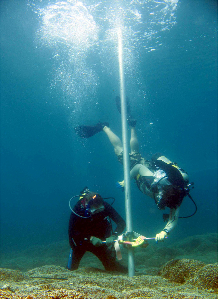
The geological epoch known as the Holocene began about 11,700 years ago, after the end of the last glacial period. In Pacific Panamá, Holocene coral reefs began growing after rising sea levels flooded shallow-water environments in the region as early as 7,000 years ago (Toth et al., 2012, 2017). Some coral reefs in the ETP preserve complete geological records of their Holocene development as frameworks of coral skeletons packed in sediments. Scientists take core samples from these reefs to collect the skeletons of corals that grew in times past (Figure 2), and they can use techniques such as radiocarbon (¹⁴C) dating to determine the times that correspond to different depths within the cores. The cores are drilled vertically through the reef structure, so younger reef material is recovered from the top of the core, and older reef material is found at the bottom of the core. The framework of coral skeletons provides ecological information on which species were growing at different times, as well as geological and chemical proxies for determining the age, rate of growth, and environmental conditions that occurred throughout the history of the reefs.

 

Figure 2. Scientists collect a coral reef core from Pacific Panamá. The core is manually forced into the reef framework using adjustable core handles and a sliding hammer weight (not shown). After the core has penetrated up to 5 m into the reef, it is capped and extracted, allowing the cored section of the reef to be recovered. Photo credit: Richard Aronson. > High res figure

 

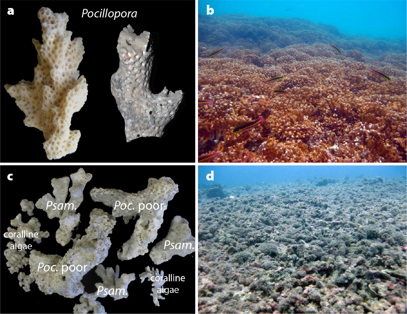
Under normal conditions for reef growth, most coral reefs in Pacific Panamá are dominated by branching corals of the genus Pocillopora; however, in more disturbed environments, the “weedy” coral Psammocora stellata or non-coral organisms such as coralline algae (red seaweeds that lay down their own skeletons of calcium carbonate) can become more abundant (Figure 3). The relative abundance of Pocillopora spp. compared with other constituents of a reef core can, therefore, provide a first indication of the past health of a reef. The taphonomic conditions, or degrees of physical degradation, of coral skeletons preserved in the geologic record provide additional information about the state of the reef in the past. Coral skeletons remain in good physical condition if they are rapidly buried after the corals die, which typically occurs when the reef is actively growing: new, living coral and fine sediment rapidly cover the dead skeletons. In contrast, when reef growth is interrupted, coral skeletons can remain on the reef surface for prolonged periods and become eroded, encrusted, or otherwise degraded (i.e., the taphonomic condition declines; Figure 3). The species composition and taphonomic condition of corals allow scientists to identify distinct layers in the cores that represent periods of active or interrupted reef growth.

 

Figure 3. Key for identifying the composition and condition of corals and coralline algae in a core. (a) Two examples of Pocillopora in good taphonomic condition (<50% erosion or encrustation of the skeleton). Intervals in cores during which Pocillopora skeletons dominate and are in good condition represent times of good coral growth and active reef development (b). (c) Example of core constituents from an interval representing poor coral growth and interrupted reef development (d). Such intervals are dominated by Pocillopora skeletons in poor taphonomic condition (“Poc. Poor”), Psammocora stellata skeletons (“Psam.”), and/or coralline algae (>50% erosion or encrustation of the skeleton). > High res figure

 

Using Physical and Chemical Evidence from Coral Reef Cores to Reconstruct Reef Growth and Environmental Variability

Coral reef accretion in Pacific Panamá was shut down for a period of ~2,500 years beginning around 4,200 years before present (yr BP; Toth et al., 2012, 2015). This hiatus in reef accretion in Panamá represents roughly 40% of the reefs’ geologic history—they began to grow 6,500 to 7,000 years ago when sea level was high enough to flood areas of the continental shelf—and marks the transition from the Middle Holocene to the Late Holocene epoch. By reconstructing past environmental conditions using a combination of coral taphonomy and geochemistry, scientists determined that the 2,500-year shutdown of coral reef development in Pacific Panamá was most likely the result of increased variability in both the frequency and intensity of ENSO events (Toth et al., 2012, 2015).

To study the long-term history of reef development in Pacific Panamá, researchers recovered reef cores from the Gulf of Panamá. Each core was divided into 5 cm vertical sections and then the constituents of each section were sorted by species for analysis. In each of those sections, the material present was identified as (1) Pocillopora, the coral that builds reefs, (2) Psammocora, a coral that does not build reefs, or (3) coralline algae that also do not build reefs. For Pocillopora corals, each skeleton was rated as being in good or poor taphonomic condition (Figure 3a,c). The scientists used this information to identify layers in the cores that were associated with periods of active reef growth (Figure 3b) based on dominance by Pocillopora in good condition, or periods during which reef growth was interrupted (Figure 3d), based on dominance by Pocillopora in poor condition, Psammocora, and/or coralline algae. Radiocarbon and other dating techniques were used to create a chronology for each core. By dividing the thickness of each layer of the core by the time period covered by that layer, rates of upward reef growth, or vertical accretion, could be reconstructed through time.

For example, the generalized core shown in Figure 4 is ~400 cm, or 4 m, long, and represents the reef framework to a depth of 4 m from the living surface of the reef. The youngest corals are at the top, and the oldest corals are at the bottom of the core. The bottom of the core dates to 6,000 yr BP, and during that time the coral in the core grew 4 m to the height when collected. Based on this knowledge, we can calculate an average accretion rate for the reef since 6,000 yr BP as 4 m/6,000 yr, or 0.67 m/1,000 yr.

 

Figure 4. Schematic representation of a core of reef framework from the Gulf of Panamá. Green shading indicates Pocillopora in good taphonomic condition, suggesting intervals of active reef growth. Gray shading indicates Pocillopora in poor condition, Psammocora, and coralline algae, all of which suggest time periods of interrupted reef growth. The hiatus (gray shading) is shown as depth in the reef framework (left) and years BP (right). Dark gray shading denotes the most conservative time span for the hiatus, and light gray shows the measured range of the hiatus. Based on dating of coral fragments, no coral was deposited in the reef framework until the end of the hiatus, hence, the absence of icons indicating coral in the drawing on the right during most of the hiatus. A key for identifying coral taphonomic condition is provided in online Handout S1. Modified from Toth et al. (2012). > High res figure

 

Scientists also measured the geochemical compositions of the corals through time by drilling skeletal fragments of Pocillopora spp. recovered from different positions within a core. The limestone powder produced by the drill was analyzed for selected elements. This allowed the scientists to reconstruct environmental conditions on the reef during three time periods: 5,000–4,500, 4,000–3,500, and 1,500–1,000 yr BP. To reconstruct the climate and ocean environmental variability of the reef through time, specialized laboratory equipment was used to measure strontium-to-calcium ratios (Sr/Ca), and barium-to-calcium ratios (Ba/Ca). The fine-scale relationships between the two elemental ratios within the coral skeletons were then compared to determine the environmental conditions that likely occurred during the lives of the corals. Corals record environmental conditions, including temperature, salinity, and water chemistry, at the time their skeletal material formed. Their chemistry can, therefore, give a chronological history of past environmental change.

Elemental ratios measured in the coral skeletons can provide powerful proxies for long-term trends in temperature and upwelling intensity. Although corals are primarily composed of calcium carbonate, other elements with the same charge (i.e., the alkaline earth metals) can replace Ca²⁺ in the coral skeleton in trace amounts. The degree to which this elemental substitution occurs depends on the environmental conditions at the time the skeleton was laid down by the coral animal. For example, strontium is substituted for calcium in the skeleton at a higher rate under cooler temperatures (i.e., higher Sr/Ca ratios are expected during cooler time periods and this trend reverses with warmer temperatures). Higher Ba/Ca ratios can represent nutrient influx associated with upwelling of cooler water and terrestrial runoff (Toth et al., 2015; LaVigne et al., 2016). El Niño conditions are associated with warmer temperatures, lower rainfall, and decreased upwelling in Pacific Panamá, so a prolonged, El Niño-like period in reef history would be indicated by lower Sr/Ca and Ba/Ca. Conversely, a prolonged La Niña-like period would be indicated by higher Sr/Ca and Ba/Ca. These elemental ratios in the coral skeletons can, therefore, be used as proxies for past ENSO variability in the ETP.

 

RESEARCH QUESTIONS AND HYPOTHESES

During this guided-inquiry exercise, students will answer three research questions about coral reefs in the Gulf of Panamá:

1. How did the taphonomic condition and species composition of past coral reefs change during the Middle to Late Holocene (Activity 1)?

2. How did the rate of reef accretion change through time, and how does it relate to changes in the composition of the coral reef cores (Activity 2)?

3. What are the relationships among the elemental ratios and environmental conditions during the Middle to Late Holocene recovered from the cores (Activity 3)?

Students will formulate hypotheses about how variability in ocean conditions or climate may have changed coral reef growth over the last 5,000 years in Activity 1. They will make comparisons of the taphonomic conditions and species compositions of coral skeletons from three core sections by characterizing the skeletons under random points. Students will then calculate changes in reef accretion through time in Activity 2, using “core logs,” which are representations of the three cores analyzed in Activity 1. Finally, in Activity 3, students will test their predictions about environmental change using mock geochemistry data: they will correlate hypothetical average elemental ratios during three time periods with predicted oceanographic conditions associated with changes in ENSO variability and the strength of upwelling in the Gulf of Panamá.

To ensure that students have a general understanding of the biology and ecology of coral reefs and ENSO variability, we encourage teachers to provide background information prior to completing the lesson, through discussion or a student-led, online scavenger hunt (e.g., https://oceanservice.noaa.gov/​education/​tutorial_corals/ and https://www.noaa.gov/​education/​resource-​collections/​weather-​atmosphere-​education-​resources/​el-nino). If time permits, we encourage teachers to supplement this lesson with other hands-on activities published in Oceanography that focus on the ecology of corals under environmental changes (Boleman et al., 2013; Gillikin et al., 2017; Gravinese et al., 2018). We also recommend that educators explore the global sea­water database with their students to help familiarize themselves with the relationship between different isotopic ratios and climatic variability (https://data.giss.nasa.gov/o18data/). We provide a glossary of terms that students can reference throughout the lesson (see Handout S1).

 

MATERIALS FOR EACH PAIR OF STUDENTS

ACTIVITY 1
• Online Student Activity Sheet
• Online Handout S1

ACTIVITY 2
• Online Student Activity Sheet
• Online Handout S1

ACTIVITY 3
• Online Student Activity Sheet
• Online Handout S1
• Mock element materials (see the online Notes for the Instructor)
     – Mock trace elements such as a type of candy with differences in mass (e.g., plain vs. peanut candies)
     – Containers to hold the mock trace elements

 

ACTIVITIES

Pre-Lab Activity

Students should review and compare the environmental and oceanographic conditions in the Gulf of Panamá under ENSO-neutral, El Niño, and La Niña climatic conditions presented in Table S1 in the Student Activity Sheet. After completing Table S1, students will answer the pre-lab questions provided.

PRE-LAB DISCUSSION QUESTIONS

The instructor can use the following questions/prompts to foster discussions that will help introduce the environmental differences that occur during ENSO-neutral, El Niño, and La Niña times. We suggest that the instructor first show the students the following animation or similar ENSO animation to help guide the student diagrams: https://oceanservice.noaa.gov/facts/ninonina.html.

1. How do the environmental parameters change in the Gulf of Panamá among ENSO-neutral, El Niño, and La Niña periods?

2. Create a diagram that explains the environmental changes that occur during ENSO-neutral, El Niño, and La Niña conditions.

 

Activity 1. Reconstructing Changes in Reef Health Using the Taphonomic Conditions and Species Compositions of Coral Skeletons in Reef Cores

SUGGESTED CLASS TIME: APPROXIMATELY 45–65 MINUTES

During this activity, pairs of students will compare the species compositions and taphonomic conditions of corals in reef cores collected from the Gulf of Panamá. Students will be given a set of digital images of corals and other material from sections sampled in the cores: three images per core, from three cores. Each core will be sampled at three time points: 1,500–1,000 yr BP, 4,000–2,000 yr BP, and 5,000–4,000 yr BP. Student pairs will do the following.

1. Use the digital images provided in Handout S1 to identify the species collected from each time interval for each core recovered (Figure 4). Each set of images will represent coral reef conditions at 1,500–1,000 yr BP, 4,000–2,000 yr BP, and 5,000–4,000 yr BP. The photographs are labeled to identify the individual cores, and the time periods within the cores are shown.

2. Overlay 15 random points onto each image using a random-​number generator, such as those available in Excel (tutorial: https://www.excel-easy.com/examples/random-​numbers.html) or Google (Google has a number generator function/calculator in the search bar), to select which points you will use. Once the random numbers have been selected, carefully cut out each of the 15 corresponding squares on the pre-made numbered core analysis grid we provide in Handout S1.

3. Use the key in Handout S1 to categorize each random point as falling on (1) Pocillopora branches in good condition, (2) Pocillopora rubble in poor condition, (3) Psammocora rubble, (4) coralline algae, or (5) other, which indicates points that do not fall on core material (these will be excluded from the analysis). The condition of Pocillopora can best be distinguished by how easy it is to see the corallites (the cups in which the coral polyps sit, visible as indentations in the surface sculpture of the skeleton): if the corallites are clear and retain their complex sculpture, the coral is in good condition; if they are more difficult to distinguish, it is in poor condition. Note that color of the coral skeleton should not be used to determine condition.

4. Calculate (1) the average percent of points that are Pocillopora in good condition, and (2) the average of the sum of points that are Pocillopora in poor condition, Psammocora, and coralline algae across the three cores for each time period. The total number of points for calculating the percentages should be the sum of the four categories above; points that do not fall on the core constituents listed should not be counted in the total.

5. Enter the data in Table S2 in the Student Activity Sheet and use these data to help answer the Activity 1 discussion questions.

6. Use the data collected in Table S2 to calculate the summary statistics for each time interval among the three cores and record the data in Table S3 in the Student Activity Sheet. Be sure to calculate the average for each time interval. Use the summary statistics to create a bar graph depicting the temporal differences observed between Pocillopora corals found in good condition and the sum of the other three categories of core constituents. After completion, use the data as evidence for answering the discussion questions for Activity 1.

ACTIVITY 1 DISCUSSION QUESTIONS

1. What temporal differences did you observe in the species of the corals present in the cores?

2. How did the corals’ taphonomic conditions change across the sampling intervals in the cores? Explain.

3. Hypothesize what may have driven the changes you observed. Explain.

 

Activity 2. Using Measurements from Reef Cores to Examine Temporal Changes in Reef Accretion

SUGGESTED CLASS TIME: APPROXIMATELY 30–45 MINUTES

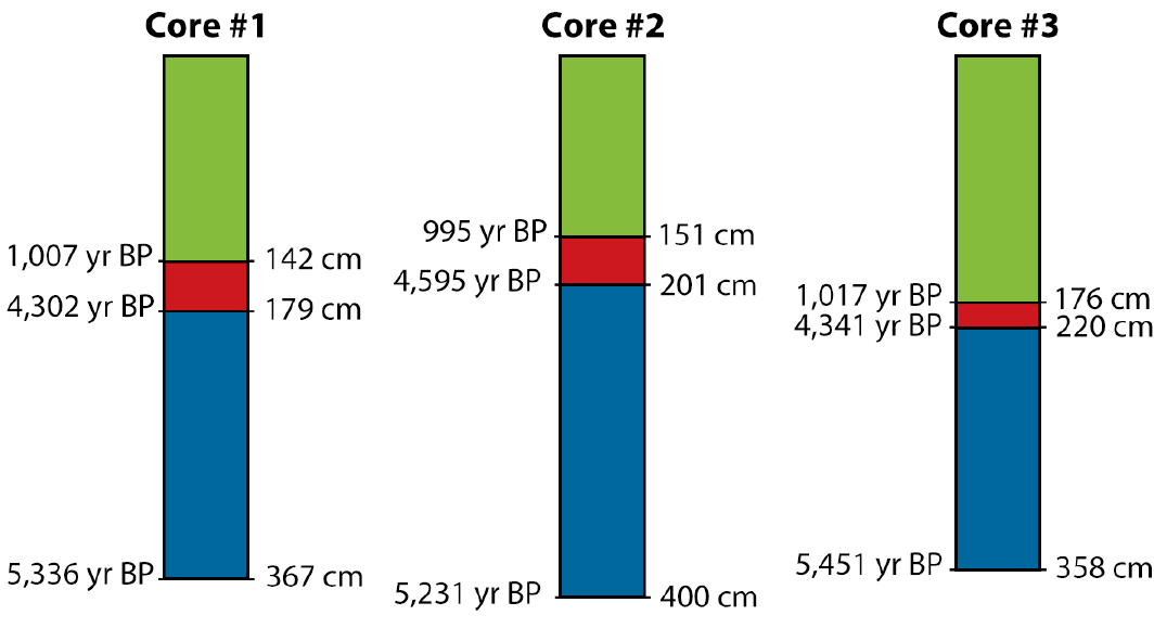
In this activity, students will work in pairs and use core logs (Figure 5) that are based on the actual cores analyzed for species composition and taphonomic condition in Activity 1. Students will calculate the length and time span of each layer observed in each core using the data provided in the graphic. Students will then use these data to calculate rates of reef accretion during three time intervals, indicated by the three colors in Figure 5. Using the accretion rates and information about the composition of the cores in the different intervals (from Activity 1), students will discuss the history of reef health and growth in Pacific Panamá through time.

 

Figure 5. Colors indicate distinct layers in the cores identified based on differences in the species composition and taphonomy of the core intervals. Ages, in years before present (yr BP) bounding those layers, are indicated on the left, and the depths of the layers in centimeters (cm) are indicated on the right. The tops of the cores should be assumed to be 0 cm and 0 yr BP. > High res figure

 

Student pairs will do the following.

1. Use the core logs provided in Figure 5 to calculate the length (in cm) and time span (years) of each interval in each idealized core.

2. Calculate accretion rates for each interval.

3. Enter the data in Table S4 in the Student Activity Sheet.

4. Calculate and plot the average accretion for each of the three time intervals. Note that although the exact time span of the intervals varies among the cores, roughly the same periods in the history of the reef are represented in all three records.

5. Use the data to answer the discussion questions for Activity 2.

ACTIVITY 2 DISCUSSION QUESTIONS

1. What changes did you observe among the sections of the cores? Describe the relationships among the core ages and core lengths.

2. Which sections of each core had the fastest accretion rate? The slowest accretion rate? Explain and defend your answer using your data as evidence.

3. Hypothesize what may have driven the changes you observed. Explain your reasoning.

 

Activity 3. Estimating Holocene Environmental Changes Using Elemental Ratios

SUGGESTED CLASS TIME: APPROXIMATELY 30–45 MINUTES

This activity is designed to have pairs of students correlate elemental ratios found within coral skeletons with inferred changes in the surrounding environment. Student pairs will count and calculate the ratios of specific elements typically found in the coral skeletons using a mock data set that simulates and models the average elemental ratios for three time periods, based on real data from the sampled cores. Each of the elemental ratios—Sr/Ca and Ba/Ca—used in this activity corresponds to a specific change in environmental conditions and serves as a proxy for changes in temperature and upwelling intensity during the life of the coral. Scientists use the Sr/Ca ratio as a proxy for temperature, whereas the Ba/Ca ratio is representative of nutrient flux associated with upwelling (Toth et al., 2015).

The teacher should prepare in advance containers filled with Sr/Ca and Ba/Ca mimics, which are described in the online Notes for the Instructor. The prepared elemental containers will represent the average element ratios of coral skeletons recovered from the cores during each time interval: 5,000–4,500, 4,000–3,500, and 1,500–1,000 yr BP. The activity will allow students to observe temporal changes in the elemental ratios similar to data recovered from an actual core and provide an opportunity to correlate the changes with environmental conditions during the life of the coral reef (e.g., upwelling vs. non-upwelling conditions, warm vs. cold temperatures). We recommend that the items used as elemental mimics represent the differences in mass among the elements being analyzed. For example, Ca has a molecular weight of 40 and could be represented by plain M&M’s®. Strontium has a molecular weight of 87 could be represented by Peanut M&M’s®. Ba has a molecular weight of 137 and could be represented by Almond M&M’s®. Alternatively, the teacher could create cardboard cutouts to represent the elemental relationships described above. The teacher should also review the lecture notes and Activity 1 with the students before beginning Activity 3.

Each student pair will be given three containers representing Sr/Ca and three containers representing Ba/Ca, with one of each type for each of the three time intervals. This activity is designed to model the trend scientists observed in the elemental ratios of a core so that students can use the data to infer what the environmental conditions were like during the lives of the corals in each interval. Student pairs will do the following for all three intervals.

1. After sorting the Sr/Ca sample, calculate the ratio of Sr/Ca for each time interval. Coral skeletons are primarily made of calcium and so several orders of magnitude more Ca would be expected to be present in a skeletal sample. To avoid having students count hundreds of Ca mimics, for the purpose of this lesson we have added a “Ca multiplier” to the actual formula used to determine the geochemical ratios. The teacher should be sure to explain to students that the amount of Ca found in the sample should be multiplied by 10.

2. Calculate the Sr/Ca ratio for each time interval and record the results in Table S5 in the Student Activity Sheet.

3. After sorting the Ba/Ca samples, calculate the ratio of Ba/Ca for each time interval in the core.

4. Calculate the Ba/Ca ratio and record the results in Table S5 in the Student Activity Sheet.

5. Use the geochemical ratios to generate hypotheses about the environmental conditions that were likely present at each time interval throughout the sampled core.

6. Revisit the data recorded in the prior activities to draw conclusions about the environmental conditions during each time interval and record ideas in Table S6 in the Student Activity Sheet.

7. Before answering the discussion questions, the instructor should summarize on the board the class’s observations from the activity.

8. Answer the discussion questions for Activity 3.

ACTIVITY 3 DISCUSSION QUESTIONS

1. What temporal changes did you observe in the Sr/Ca ratio? The Ba/Ca ratio?

2. The magnitudes of the observed changes are small, but they provide a lot of information about past climate. Based on the small changes observed, what do the environmental conditions you inferred suggest about the impacts of environmental changes on the health and growth of coral reefs in the Gulf of Panamá? Use the summarized data from the class observations for this activity. Support your answer with evidence from the lab activities.

 

ACKNOWLEDGMENTS

We thank C. Randall, P. Barrett, M. Costa, A. Dwyer, R. Fidler, J. Leichter, D. Stein, E. Whitcher, S. William, B. Steffel, and A. Zamora-Duran for their assistance during this project. PMG’s postdoctoral fellowship at Mote Marine Laboratory and Aquarium was supported by the Steinwachs Family Foundation. Funding was provided by grant OCE-1535007 from the US National Science Foundation, and by the Coastal/Marine Hazards and Resources Program of the US Geological Survey. Data were collected under permit #SC/AO-3-16 from MiAmbiente, Republic of Panamá. Any use of trade, firm, or product names is for descriptive purposes only and does not imply endorsement by the US government. Finally, we thank four reviewers, whose comments improved the clarity of this lesson. This is contribution number 224 from the Institute for Global Ecology at the Florida Institute of Technology.

Gravinese, P.M., R.B. Aronson, and L.T. Toth. 2020. Digging into the geologic record of environmentally driven changes in coral reef development. Oceanography 33(1):85–91, https://doi.org/10.5670/oceanog.2020.113.

» Student Activity Sheet (264 KB pdf)

» Handout S1 (6.9 MB pdf)

» Notes for Instructor (59 KB pdf)

» Answer Key (72 KB pdf)

Anthony K.R.N., S.R. Connolly, and O. Hoegh-Guldberg. 2007. Bleaching, energetics, and coral mortality risk: Effects of temperature, light, and sediment regime. Limnology and Oceanography 52(2):716–726, https://doi.org/10.4319/lo.2007.52.2.0716.
1. Aronson, R.B., W.F. Precht, I.G. Macintyre, and T.J.T. Murdoch. 2000. Coral bleach-out in Belize. Nature 405:36, https://doi.org/10.1038/35011132.
2. Boleman, C.L., P.M. Gravinese, E.N. Muse, A.E. Marston, and J.G. Windsor. 2013. Corals on acid: An inquiry-based activity leading students to a better understanding of ocean acidification impacts. Oceanography 26(4):164–169, https://doi.org/10.5670/oceanog.2013.87.
3. Cohen, A.L., and M. Holcomb. 2009. Why corals care about ocean acidification: Uncovering the mechanism. Oceanography 22(4):118–127, https://doi.org/​10.5670/oceanog.2009.102.
4. Costanza, R., R. De Groot, P. Sutton, S. Van der Ploeg, S.J. Anderson, I. Kubiszewski, S. Farber, R.K. and Turner. 2014. Changes in the global value of ecosystem services. Global Environmental Change 26:152–158, https://doi.org/​10.1016/j.gloenvcha.2014.04.002.
5. Garrison, T.G. 2013. Pp. 247–263 in Oceanography: An Invitation to Marine Science, 8^th ed. Brooks Cole/CEngage Learning, Belmont, CA.
6. Gillikin, D.P., A. Verheyden, and D.H. Goodwin. 2017. Paleoclimate reconstruction from oxygen isotopes in a coral skeleton from East Africa: A data-enhanced learning experience. Oceanography 30(1):104–107, https://doi.org/10.5670/oceanog.2017.104.
7. Glynn, P.W. 1977. Coral growth in upwelling and nonupwelling areas off the Pacific coast of Panama. Journal of Marine Research 35(3):567–585.
8. Glynn, P.W. 1993. Coral reef bleaching: Ecological perspectives. Coral Reefs 12(1):1–17, https://doi.org/10.1007/BF00303779.
9. Glynn, P.W., and I.G. Macintyre. 1977. Growth rate and age of coral reefs on the Pacific coast of Panamá. Proceedings of the 3^rd International Coral Reef Symposium, Miami 2:251–259.
10. Glynn, P.W., and M.W. Colgan. 1992. Sporadic disturbances in fluctuating coral reef environments: El Niño and coral reef development in the eastern Pacific. American Zoologist 32(6):707–718, https://doi.org/10.1093/icb/32.6.707.
11. Glynn, P.W., A.B. Mones, G.P. Podestá, A. Colbert, and M.W. Colgan. 2017. El Niño–Southern Oscillation: Effects on eastern Pacific coral reefs and associated biota. Pp. 251–290 in Coral Reefs of the Eastern Tropical Pacific. Springer, Dordrecht.
12. Gravinese, P.M., L.T. Toth, C.J. Randall, and R.B. Aronson. 2018. How do upwelling and El Niño impact coral reef growth? A guided, inquiry-based lesson. Oceanography 31(4):184–188, https://doi.org/10.5670/oceanog.2018.424.
13. Hoegh-Guldberg, O., P.J. Mumby, A.J. Hooten, R.S. Steneck, P. Greenfield, E. Gomez, C.D. Harvell, P.F. Sale, A.J. Edwards, K. Caldiera, and others. 2007. Coral reefs under rapid climate change and ocean acidification. Science 318(5857):1,737–1,742, https:/doi.org/10.1126/science.1152509.
14. Hughes, T.P., K.D. Anderson, S.R. Connolly, S.F. Heron, J.T. Kerry, J.M. Lough, A.H. Baird, J.K. Baum, M.L. Berumen, T.C. Bridge, and D.C. Claar. 2018. Spatial and temporal patterns of mass bleaching of corals in the Anthropocene. Science 359(6371): 80–83, https://doi.org/10.1126/science.aan8048.
15. LaVigne, M., A.G. Grottoli, J.E. Palardy, and R.M. Sherrell. 2016. Multi-colony calibrations of coral Ba/Ca with a contemporaneous in situ seawater barium record. Geochimica et Cosmochimica Acta 179:203–216, https://doi.org/10.1016/​j.gca.2015.12.038. 
16. Lesser, M.P., and J.H. Farrell. 2004. Exposure to solar radiation increases damage to both host tissues and algal symbionts of corals during thermal stress. Coral Reefs 23(3):367–377, https://doi.org/10.1007/s00338-004-0392-z.
17. Lirman, D., S. Schopmeyer, D. Manzello L.J. Gramer, W.F. Precht, F. Muller-Karger, K. Banks, B. Barnes, E. Bartels, A. Bourque, and J. Byrne. 2011. Severe 2010 cold-water event caused unprecedented mortality to corals of the Florida reef tract and reversed previous survivorship patterns. PLoS One 6(8), https://doi.org/​10.1371/journal.pone.0023047.
18. Manzello, D.P., J.A. Kleypas, D.A. Budd, C.M. Eakin, P.W. Glynn, and C. Langdon. 2008. Poorly cemented coral reefs of the eastern tropical Pacific: Possible insights into reef development in a high-CO₂ world. Proceedings of the National Academy of Sciences of the United States of America 105(30):10,450–10,455, https://doi.org.10/1073/pnas.0712167105.
19. Moberg, F., and C. Folke. 1999. Ecological goods and services of coral reef ecosystems. Ecological Economics 29(2):215–233, https://doi.org/10.1016/S0921-8009(99)00009-9.
20. Randall, C.J., L.T. Toth, J.J. Leichter, J.L. Maté, and R.B. Aronson. 2020. Upwelling buffers climate change impacts coral reefs of the tropical eastern Pacific. Ecology 101(2):e02918, https://doi.org/10.1002/ecy.2918.
21. Roberts, H.H., L.J. Rouse, N.D. Walker, J.H. and Hudson. 1982. Cold-water stress in Florida Bay and northern Bahamas: A product of winter cold-air outbreaks. Journal of Sedimentary Research 52(1): 145–155, https://doi.org/​10.1306/​212F7EFA-2B24-11D7-8648000102C1865D.
22. Toth, L.T., R.B. Aronson, S.V. Vollmer, J.W. Hobbs, D.H. Urrego, H. Cheng, I.C. Enochs, D.J. Combosch, R. van Woesik, and I.G. Macintyre. 2012. ENSO drove 2500-year collapse of eastern Pacific coral reefs. Science 337(6090):81–84, https://doi.org/10.1126/science.1221168.
23. Toth, L.T., R.B. Aronson, K.M. Cobb, H. Cheng, R.L. Edwards, P.R. Grothe, and H.R. Sayani. 2015. Climatic and biotic thresholds of coral-reef shutdown. Nature Climate Change 5(4):369–374, https://doi.org/10.1038/nclimate2541.
24. Toth, L.T., I.G. Macintyre, and R.B. Aronson. 2017. Holocene reef development in the tropical eastern Pacific. Pp. 177–201 in Coral Reefs of the Eastern Pacific: Persistence and Loss in a Dynamic Environment. P.W. Glynn, D.P. Manzello, and I.C. Enochs, eds, Springer-Verlag, New York, https://doi.org/​10.1007/978-94-017-7499-4_6.
25. Williams, E.H., P.J. Bartels, and L. Bunkley-Williams. 1999. Predicted disappearance of coral-reef ramparts: A direct result of major ecological disturbances. Global Change Biology 5(8):839–845, https://doi.org/10.1046/j.1365-2486.1999.00272.x.
26. Wyatt, A.S.J., J.J. Leichter, L.T. Toth, T. Miyajima, R.B. Aronson, and T. Nagata. 2019. Heat accumulation on coral reefs mitigated by internal waves. Nature Geoscience 13:28–34, https://doi.org/10.1038/s41561-019-0486-4.

This is an open access article made available under the terms of the Creative Commons Attribution 4.0 International License (https://creativecommons.org/licenses/by/4.0/), which permits use, sharing, adaptation, distribution, and reproduction in any medium or format as long as users cite the materials appropriately, provide a link to the Creative Commons license, and indicate the changes that were made to the original content. Images, animations, videos, or other third-party material used in articles are included in the Creative Commons license unless indicated otherwise in a credit line to the material. If the material is not included in the article’s Creative Commons license, users will need to obtain permission directly from the license holder to reproduce the material.