
Full Text
Purpose of Activity
Collecting data in the ocean requires scientists to choose, use, and interpret the output of sensor-based instruments. With the increasing accessibility of do-it-yourself (DIY) technology, researchers are able to develop innovative and cost-effective instruments with relative ease compared to just 10 years ago. As part of a project-based course to teach undergraduates and graduate students engineering skills that are useful in marine science, we developed an Arduino-based instrument to measure temperature and depth. By building, calibrating, and testing this instrument, students learn about sensors and circuits, are introduced to hardware and software design, and collect, analyze, and interpret their own data. More broadly, students learn principles of instrument design and develop problem-solving skills.
Audience
This project takes approximately half the semester (~8 weeks) of a course for undergraduates and graduate students. In our class, students spend the rest of the semester on independent projects. This instrument design allows for adding or swapping sensors to fit the interests, time constraints, and level of expertise of the students. The instructions are written assuming minimal experience in engineering, so it would likely be appropriate for high school or beginning undergraduates. The project-based nature of our course allows students to move through the material at their own pace, which works well for the varied backgrounds of our students.
Background
In most areas of science, we use sensors to measure environmental variables such as temperature, oxygen, pH, wind, or current velocity, and, in marine/aquatic environments, conductivity and water depth. These measurements are increasingly important under global climate change, as flooding, storm surge, and wind events are expected to increase in frequency, and temperature is expected to increase in magnitude and variability (Pershing et al., 2018). These variables are commonly measured in conjunction with other environmental or ecological variables. Many marine scientists use off-the-shelf instruments to measure these parameters, but how these instruments function can seem mysterious. With advances in open-source technology comes the potential to develop new instruments to measure the environment and answer new questions (Butler and Pagniello, 2021). Additionally, sensors and instruments are being developed with higher resolution and precision that often comes at increased cost, and scientists need the expertise to understand these trade-offs and choose the best instrument for a specific application. An understanding of the functioning of an instrument can help researchers use them more effectively, understand instrumentation limitations and why they exist, and troubleshoot issues when they inevitably arise.
We have developed and taught a course, entitled Marine Technical Methods, that provides undergraduates and graduate students with basic engineering skills as well as critical thinking and problem-solving capabilities (Boss and Loftin, 2012). During the first half of this semester-long course, students build a submersible, Arduino-based instrument to measure water temperature and depth (the Temperature Depth datalogger, TDd). The second half of the semester, based on their own personal or research interests, the students are asked to use the knowledge they gained to create their own devices using the technological principles they learned in building the TDd. Project-based learning, in which students learn curriculum concepts through a project, provides intrinsic motivation and helps create independent thinkers and learners (Bell, 2010).
Initially, the students are exposed to the basics of circuits and how sensors work. As their knowledge grows, they are gradually introduced to programming in Arduino and MATLAB, and then to more advanced topics (i.e., basic principles of underwater housings). Eventually, they assemble and calibrate their own TDd, which they deploy twice. First, the TDd is deployed as a “long-term” datalogger, sampling every ~5 minutes to measure tidal height and water temperature over several days. The next deployment is as a castable profiling instrument: sampling as fast as possible, their instruments are lowered from the surface to approximately 15 m depth. The data from each deployment are compared to reference data sets. The long-term deployment references a hydrographic and weather station (https://www.disl.edu/arcos/), and the profiling data set references a Sea-Bird SBE25plus CTD. The students use MATLAB to manage and analyze the data and are asked to draw conclusions about the performance of their instruments in both situations. Students develop an understanding of how sensors respond to the environment and are better able to evaluate design options and assess when and to what extent data can be trusted.
Project Overview and Materials
Students complete the TDd project (Figure 1) as four parts, each of which takes about two to four three-hour class periods and includes a project report: (1) temperature sensor (introduction to circuits and sensors), (2) pressure sensor (building knowledge of circuits and sensors), (3) building the instrument (assembly of electronics, compiling code, and powering and finishing housing), and (4) collecting and analyzing the data. Detailed instructions are provided in the online supplementary Appendix S1. Each instrument costs ~$200, but instruments can be disassembled and rebuilt with minimal (<$20) consumable costs (Table S1).
|
|

Parts 1–2: Temperature and Pressure Sensors
ELECTRONICS
An Arduino Uno microcontroller with an Adafruit Data Logger Shield is used to read and log data from the two sensors to an onboard SD card. A temperature sensor is created from a 10 kΩ thermistor (Adafruit), and water depth is measured with a 0.2 MPa 4–20 mA pressure sensor. The 10 kΩ thermistor is used in a voltage divider circuit designed to use the 5 V output pin from the Arduino to output 0–5 V that is read through an analog input terminal of the Arduino. Students apply Ohm’s law to select the resistance value for the other (pull-down) resistor in the circuit. The 0.2 MPa pressure sensor selected allows for measurements to 20 m depth. The 4–20 mA output requires students to apply Ohm’s law to calculate the resistance needed to convert the current output of the sensor to a voltage (0–5 V) that the Arduino Uno can read through an analog input terminal. Both sensors are wired to separate analog input terminals in the Arduino Uno. After assembling and testing on a breadboard, circuits are transferred and soldered onto a perf-board (Figure 1). Although the Data Logger Shield has a small circuit prototyping area that could be used, we opted for a Breadboard PCB perf-board that had more space. In addition, the similar layout to a breadboard makes the prototyping PCB more intuitive for students to use. The instrument is powered with eight AA batteries wired in series to produce an output of 12 vdc, but with limited battery life of 24–48 hours. The 12 V power source powers the pressure sensor and Arduino directly and is also regulated down to 5 V by the Arduino’s onboard voltage regulator. The Arduino’s 5 vdc output is used to power the thermistor circuit. Electronic components are mounted on a 2.5 × 10 × 0.125 inch thick acrylic sheet that is later trimmed to fit inside the waterproof housing (Figure 1).
CODE
Students initially modify example Arduino code to complete specific tasks and build their programming skills, then they combine their codes. In part 1, they read the analog input for the temperature sensor circuit and use the real-time clock to log data to the SD card. Then in part 2, they read the analog input for the pressure sensor through a different analog input pin (see instructions in Appendix S1). Next, in part 3, they combine these components into one code to read and log real time, temperature, and pressure in a continuous loop. Data are logged on an SD card in .csv format, to be imported for analysis in MATLAB. Because this is a teaching tool, the completed code assignment is not publicly available, but is available by request from the authors.
CALIBRATION
Students calibrate the pressure sensors (part 2) using tubing with water at different heights (h), from which pressure (P) is calculated using the hydrostatic equation:
P = ρgh,
where ρ is water density and g is the gravitational constant. Pressure is plotted as a function of the reading from the pressure sensor circuit, and the linear fit is used to calculate pressure from the sensor reading value. A detailed description of the pressure sensor calibration is included in Appendix S1.
The Steinhart-Hart equation is used to convert resistance of the thermistor (R) to temperature (T):
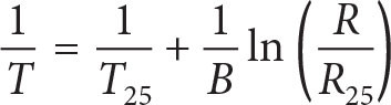 |
using the resistance of the thermistor at 25°C (R25 = 10 kW), room temperature in Kelvin (T25 = 298.15 K), and the coefficient of the thermistor (B = 3950). This is done in part 3 of our course, once students have been introduced to programming; some students who are comfortable programming choose to do these calculations during part 1.
Part 3: Preparing for Field Deployment
HOUSING
The waterproof housing is built from transparent acrylic tubing (4.125-inch OD, 0.25-inch wall thickness, 12-inch length) with end caps fabricated from acetal (Delrin) with 0.375-inch-thick cast acrylic covers with holes for sensors (Figure 1). The end caps use –237 O-rings to create the radial housing seal and –235 O-rings to make the axial seals (Figure 1). Caps were fabricated (outside of class time) in the Dauphin Island Sea Lab machine shop and custom fit to each acrylic tube following ISO3601 (groove dimensions for static axial and radial applications; https://hitechseals.com/). Cap covers are cut from acrylic using a 100-watt CO2 laser cutter. The students are asked to locate, drill, and tap holes for the temperature and pressure sensors. The pressure sensor requires a ¼-19 BSPP tapped hole, which is sealed with a face (radial) gasket against the inside wall of the acrylic cap cover. The temperature sensor uses a stainless steel thermowell, which requires a ½ NPT tapped hole. Hole locations for the sensors are critical because of space constraints inside the housing (Figure 1). CAD files are available at https://grabcad.com/library/diy_oceanography_tdd-1.
BATTERY POWER
Students use multimeters to measure the current draw of their instruments and calculate the predicted battery life of their eight AA batteries in series. They test their predictions during their deployment.
Part 4: Field Deployment and Data Analysis
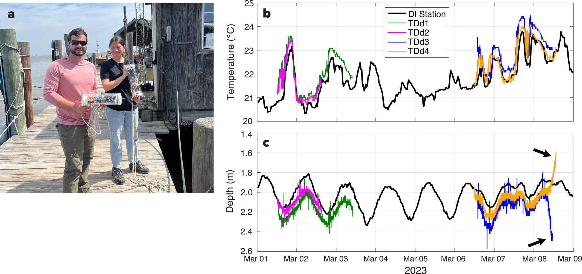
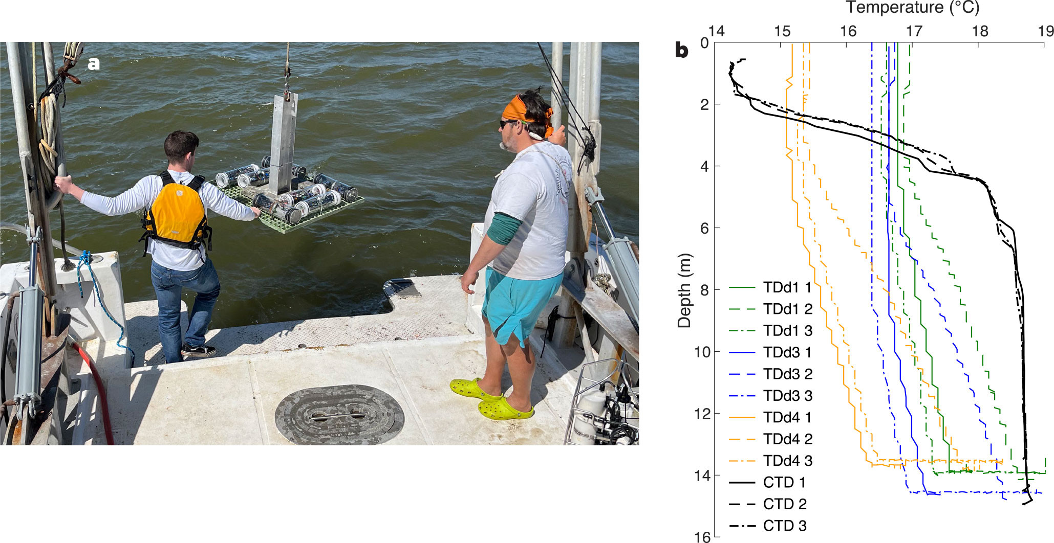
The instrument was originally developed to measure tidal height and temperature over a tidal cycle. The instrument is deployed from the Dauphin Island Sea Lab boat dock (Figure 2a), ~170 m from the Dauphin Island long-term monitoring station (https://arcos.disl.org/), where a YSI EXO 2 Sonde is deployed. Data from the students’ TDd are compared to the station data. In the class, the instrument is also tested in vertical profiling mode deployed from a boat in the Mobile Bay channel (~15 m deep), and data are compared to those from a Sea-Bird SBE25plus CTD (Figure 3a).
Students use MATLAB to plot, evaluate, and compare the data from their instruments to those from the Dauphin Island long-term monitoring station. They calculate the resolution of both sensors (determined by the 10-bit analog-to-digital converter of the Arduino Uno), then examine their data to find the actual resolution and assess the performance of the instrument. Long-term deployment data match those from the monitoring station well (Figure 2b,c). As seen in Figure 2c (black arrows), data from the pressure sensor often drift as the battery voltage drops below the required 12 vdc. The students are prompted to identify this problem and brainstorm solutions.
|
|
To deploy in profiling mode, students increase the sampling rates of their instruments. Comparison of the data collected with the students’ instruments to those of the CTD showed much greater discrepancy, but we found that troubleshooting this discrepancy is a powerful teaching tool. Many students initially struggle with the concept that they built an instrument that does not work, but they learn to identify the specific problem and brainstorm a solution. Students evaluate the performance of their instruments by assessing whether the resolution of both temperature and depth sensors (determined by the analog-to-digital converter in the Arduino), the temporal logging interval, and the response time of the sensors are sufficient to capture the temperature profile from the CTD. To help with this troubleshooting, the students’ TDd instruments are deployed three times in the Mobile Bay channel: (1) at free-fall speed, (2) at a slower drop speed, and (3) at free-fall speed but then left on the bottom for a short period (Figure 3b). Students plot and compare these three data sets to one another and to CTD casts collected immediately after each TDd profile (all at free-fall; Figure 3b) and evaluate their results. None of the TDd instruments capture the thermocline in the CTD data, which show a cold-water lens on top of warmer water, commonly observed in spring in Mobile Bay, Alabama, which is a river-dominated system (Dzwonkowski et al., 2011). The TDd temperature measurements increase more steeply when the instrument is dropped more slowly (Figure 3b, #2), and temperature continues to increase over the ~1 minute that the TDd was left on the bottom (Figure 3b, #3). Through this structured troubleshooting, students reach the conclusion that the response time of the temperature sensor is too slow for this application, but the instrument works well as long as the temperature change occurs over a long enough time compared to that response time.
|
|
Possible Modifications
In our class, after completing this project, students choose independent or group projects, many of them built off of this project. The TDd instrument was designed to be versatile, and different sensors can be added or existing sensors can be easily replaced. Students in our class have swapped the Adafruit thermistor and thermowell for a smaller thermistor with better response time (Figure S1), added a light transducer, and incorporated Atlas Scientific dissolved oxygen and conductivity sensors. Adding additional sensors becomes challenging when the housing needs to be modified (so a light sensor is the simplest of these). The housing was designed with two end caps to mount instrumentation, but any additional holes for sensors should be mounted in a bulkhead that threads into the acrylic cover and creates a static O-ring seal following established specifications (see https://hitechseals.com/ and/or ISO3601). For better resolution, the Arduino Uno microcontroller could be replaced with a microcontroller that has better analog-to-digital resolution such as the Arduino Zero or Teensy, but for teaching, the Uno offers the advantages of ease of use and low cost. A digital temperature sensor (e.g., Dallas One-Wire) may be simpler to set up, or a pressure sensor with mV output could be used with an amplifier (e.g., INA125p) for better resolution.
LONG-TERM DEPLOYMENT
As designed, the eight AA batteries last for 24–48 hours, which works well for educational purposes but is too short for most research applications. The easiest solution would be to switch to lithium batteries or commercially available, rechargeable power tool batteries (i.e., Milwaukee M18). Another option would be to use an external power supply and tether the instrument, which might be appropriate, for example, for deployment from a dock.
CAST DEPLOYMENT
To increase the response time of the temperature sensor, the thermal mass of the sensor needs to be smaller. One student solved this problem by designing and building a custom bulkhead to hold a smaller glass-sealed thermistor (MF58 10 kΩ NTC) that replaced the thermowell (Figure S1).
HOUSING
A simpler and less expensive housing could be created by gluing a PVC end cap onto one end of the PVC pipe after mounting the sensors on the end cap. The other end of the PVC pipe could be sealed with a low pressure, removable waste/vent cap. This would be less versatile but cheaper and reusable, would not require a machine shop, and would be waterproof enough for nearshore deployments (e.g., not exceeding ~4 psi).
Instrument Development as a Teaching Tool
This project has several advantages as a teaching tool. For instructors, the level of student engagement far surpasses that of any previous course, similar to observations by Boss and Loftin (2012) in their class that served as a model for ours. Students take ownership of their instruments, ask lots of questions, and stay after class to keep working. This enthusiasm likely stems from the hands-on nature of the project, the long-term investment that the students make (~½ semester), and the tangible product.
Students have been so engaged in the data analysis and evaluation of instrument performance that we opted to keep the “problems” with the initial design and spend more time in class identifying and brainstorming solutions to the problems. Through this evaluation process, students learn about the iterative process of design as well as how to understand and interpret the component specifications when choosing an instrument to address future research questions. By seeing real examples of sensor drift and of instruments “working” differently in different contexts, they also learn when and to what extent to trust their data. They also develop an understanding of how the scientific question shapes the decisions made in experimental design and, more broadly, how scientists and engineers collaborate to develop new tools to study our changing oceans. Students who have taken this class have developed new instrumentation that they have presented at conferences and will be published in the peer-reviewed literature (Cho et al., 2022; Ballentine, 2023), and others have developed new interests (e.g., in programming) that shape their future career choices.