Measuring net community production (NCP) is a challenging, yet important, aspect of oceanography. Methods based on discrete sample collection often have low spatial and temporal resolution, while expensive instruments are required to obtain continuous NCP measurements at high resolution. To address these issues, Izett and Tortell (2020) created a novel, autonomous system called the Pressure of In-situ Gases Instrument (PIGI) and shared their design with the community. The system yields high-resolution surface water O₂ and N₂ measurements that are used to estimate NCP along a ship transect or at a fixed field station. This article provides a description of an updated PIGI system that was tested in a series of cruises in the coastal South Atlantic Bight (SAB). The data collected suggest that it performs equally as well as the original, providing high spatial resolution NCP measurements. Unfortunately, we believe that the SAB coastal and estuaries violate the steady state assumption due to horizontal mixing driven by tidal forces. Thus, we cannot recommend the PIGI system for use in the coastal SAB, but we encourage its use in open ocean waters that do not violate the assumptions on which this system was built. We document the updates to the PIGI system, share tips and tricks on its use, and discuss the data collected.

Introduction

Net community production (NCP) and primary production are two key metrics for assessing the biological carbon cycle. Primary production draws down carbon and releases oxygen, while respiration does the inverse. The balance between primary production and respiration within the water is NCP (Stanley et al., 2010). NCP is challenging to quantify, and the community has come up with several proxies, such as measurements of O₂ surface variability (Kaiser et al., 2005), carbon dioxide to oxygen ratios (Laws, 1991), satellite remote sensing (Tilstone et al., 2015), and various measures of oxygen changes due to biology (e.g., Schulenberger and Reid, 1991; Emerson, 1987, 2014; Emerson et al., 1999), including quantification of O₂/Ar to correct for physical effects on O₂ saturation states (Craig and Hayward, 1987). The O₂/Ar-based methods have the potential to provide estimates of NCP integrated over ecologically meaningful temporal and spatial scales (one to two weeks, depending on the residence times of gases in the mixed layer, and 60–180 m spatial resolution, assuming a ship speed of 12 knots; Kaiser et al., 2005; Reuer et al., 2007).

The Pressure of In-situ Gases Instrument (PIGI) system was developed to measure O₂/N₂ ratios at high resolution and to derive NCP (Izett and Tortell, 2020). The system relies on the same principles as the commonly applied O₂/Ar method for NCP calculations, where NCP is estimated to be proportional to O₂/Ar in the mixed layer after accounting for sea-air exchange. While Ar measurements typically require mass spectrometry, the N₂ method is cheaper and easier to measure, as it can be derived from simultaneous total dissolved N₂ gas pressure and oxygen optode (OO) measurements (McNeil et al., 2005). Similar to O₂/Ar sampling, the PIGI system’s NCP estimates assume that N₂, like Ar, is a biologically inert analog for O₂, meaning that the O₂/N₂ ratio is unaffected by temperature and salinity-​dependent solubility effects, and that there is no biological impact on N₂. Izett and Tortell (2021) and Izett et al. (2022) tested the validity of these assumptions in model and field tests, demonstrating a negligible impact of biological N₂ cycling on mixed layer O₂/N₂ signals. They also found near-equivalence between surface O₂/Ar- and O₂/N₂-derived NCP estimates. As a result, Ar can be replaced with N₂, enabling the use of O­₂/N₂ as a low-cost NCP tracer.

Izett and Tortell (2020) published full details of the hardware and software designs for the PIGI system, supporting its use by the community. Their system contains an oxygen optode and gas tension device and operates using automated data acquisition software. Following Izett and Tortell (2020), we built a revised PIGI system that incorporated several significant improvements. Our tests of the revised system took place in the coastal South Atlantic Bight (SAB), an ocean region known to be heterotrophic in the estuaries and autotrophic offshore (Hopkinson, 1985; Hopkinson et al., 1991). The net heterotrophic condition in the estuaries results from the export of organic carbon from coastal salt marshes (Hopkinson 1985; Hopkinson et al., 1991; Signorini et al., 2005), which stimulates bacterial respiration and creates a net O₂ sink in the estuaries. This water is exported to the nearshore region by tides and winds. The O₂ saturation state in the SAB is also seasonal, with warmer periods associated with undersaturation (Jiang et al., 2010). The combination of these various processes results in complex NCP dynamics in the SAB, making it an ideal region for testing the PIGI system. Here, we present a deployment of the PIGI in the SAB region and describe the modifications we made, evaluate data from a deployment, and discuss tips and tricks. We hope that this update will help support the community in using this system and lower barriers to its further development.

 

PIGI Modification

We made four modifications to the PIGI system to improve its functionality: (1) made the OO chamber watertight, (2) updated the CAD files so that instrument decals were accounted for, (3) rewired the OO to provide more robust power, and (4) updated the acquisition software to improve performance and OO model compatibility. These modifications, shown in Figure 1a, were made with the best practices for optical flow through systems in mind (Boss et al., 2019). Updated CAD files, drawings, acquisition software, and software setup guide can be found online at https://doi.org/​10.5281/zenodo.4024951. We believe that the system is now easier to build, and the software offers an improved user experience.

 

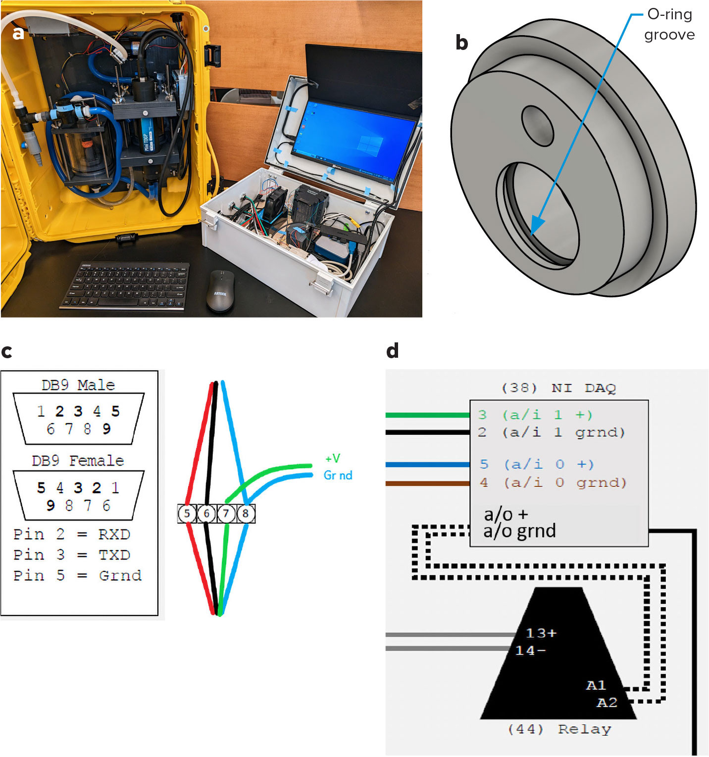
FIGURE 1. Design updates to the Pressure of In-situ Gases Instrument (PIGI). (a) View of the updated PIGI system. (b) O-ring groove added to Part I (see design drawings at https://doi.org/10.5281/zenodo.4024951), location indicated by blue arrow. (c) Update for oxygen optode to 12 V power source (red – TXD, black – RXD, green – positive volts, blue – ground). (d) Updated wiring on the relay diagram for the National Instruments Data Acquisition unit for the pump. > High res figure

 

1. Making the oxygen optode chamber watertight.

We found that the original design leaked around the OO. We opted to seal it by installing an O-ring in Part I (see Figure 1b), which involved modifying the original design by cutting a new groove in the optode hole.

The O-ring groove is included in the updated CAD files. Briefly, the groove is 1/8 inch above the inside face of Part I. It is cut 0.165 inches wide and 0.118 inches deep. The suggested tolerances for the CAD files have been updated to +.005/–0 inches for slip fits and ±0.10 inches for holes that will be national pipe thread (NPT). These tolerances have been applied across the board. The dimensions for the O-ring groove were chosen so that modifications can be made to existing PIGI systems and take an already used O-ring size, part 13 in Izett and Tortell (2020).

2. Updating the CAD drawings.

Both the two-dimensional drawings and three-​dimensional CAD files have been updated. The update resolves some inconsistencies between the files and updates the manufacturing design for the system. The inconsistencies mostly involved hole sizes for the American national pipe standard, more commonly called NPT taps. An NPT tap is the standard screw separation distance and angle for both male and female screws in the United States. The original CAD drawings did not have the NPT taps included and were indicated as the maximum tap width. If taps are cut to maximum width, the screw aspect cannot be threaded and would have required a full re-cut if not caught (potentially $4,000). Additionally, a few holes appeared on the CAD drawings, but not on the technical drawings. Manufacturing improvements included the removal of some unnecessary cuts and the redesign of some others to reduce manufacturing difficulty.

Another update to the CAD files was related to the decals containing the serial and model numbers on the instruments that caused them to be larger than the manufacturer specification. The University of Georgia’s equipment policy and the warranty for the equipment require keeping decal information. Moreover, instrument serial and model numbers enable researchers to maintain traceable information on instruments and relevant calibration data. As removing the stickers was not an option, we modified the PIGI system to fit the decals. Size corrections were made to the optode chamber inflow cap (Part J) and the optode support (Part K).

We also note that acrylic tubes have various thicknesses, even within one tube. This makes cutting the right size for the caps slightly challenging. Measuring the inner diameter of the tubes prior to cutting PVC can be very helpful.

These changes aim to decrease the manufacturing difficulty and prevent costly mistakes. The manufacturing changes we introduced decrease the number of molds needed to accurately cut the PVC and remove unnecessary directional and blade changes, simplifying the overall manufacturing process. A full list of all the changes can be found at https://zenodo.org/records/7776382.

3. The oxygen optode was rewired to supply more robust power to the optode.

The original wiring provided power from a USB cable power source. We rewired the OO with the power cable coming directly to a 12VDC/4.5A power source (an additional part 42 from Izett and Tortell, 2020; see Figure 1c). We chose to add an additional 12V power source so that the power draw from the optode (5–14 V) did not lead to voltage changes in the flow meters, which could potentially affect their measurements. To make this adjustment, the power supply positive should connect straight to the positive voltage OO wire and the negative wire should connect to both the ground OO wire and the ground wire for the DB9 (see Figure 1c). Both of these connections can be made with a quick connect screw terminal. This change brings the OO power supply in line with the TDGP, which has its own power supply from 110/220 V.

4. The acquisition software was updated to be compatible with different OO models.

The custom-made PIGI acquisition software provided by Izett and Tortell (2020) was only compatible with the standard response time (~8 s) Aanderaa 4330 OO. In our system, we used the fast-response model (~1 s response time; Aanderaa 4330f); alternative OOs, such as the Aanderaa 4531 or 4835, or RBRcoda T.ODO, can also be used for cost savings. As a result, we have updated the acquisition software to be compatible with these different OO models. While the purchase of an annual LabVIEW subscription is required to edit the acquisition program, a cost-free runtime executable application is available to download onto Windows computers (available at https://doi.org/10.5281/zenodo.4024951). The runtime application allows users to specify their system setup parameters (e.g., OO type, sampling rate), and to autonomously view and log data in real time at no additional expense above the system’s hardware requirements. We provide a setup guide for the updated software in the online supplementary materials and at https://zenodo.org/records/7776382.

 

Deployment

We tested the modified PIGI system on several cruises in the SAB. Here, we present a portion of a cruise on R/V Savannah in September 2023, with the instrument continuously deployed and oxygen validation samples taken. The cruise headed directly offshore from the Skidaway Institute of Oceanography near Savannah, Georgia, out to a depth of 50 m on the continental shelf. To test the changes to the instrument, we are only showing the outgoing leg of the cruise past 15 km offshore, where the instrument is not strongly affected by tidal mixing. We are not showing the return leg, which was affected by a storm with wind speeds over 17 m s^–1. This most likely led to bubble injection, causing the return leg to produce erroneous data. During this cruise, data from 13 CTD casts portrayed vertical profiles between the surface and 50 m depth, indicating that the water column between these depths was well mixed (density change <0.5 kg m^–3).

During the cruise, we compared oxygen measurements taken from the ship’s seawater line against surface bottle samples to evaluate any potential discrepancies resulting from the ship’s sampling system (Figure 2a; Izzet and Tortell, 2021; Cynar et al., 2022; Izett et al., 2022). This was done using Winkler titrations (Culberson, 1991; Dickson, 1994) of triplicate samples taken from the inline system and from a Niskin bottle at 3 m, which is the same depth as the seawater intake location on the hull. These two datasets matched perfectly except for one point at hypoxic levels in the estuaries where the inline system showed higher oxygen. This may be caused by the inline system adding bubbles or by the presence of hydrogen sulfides in the estuaries, which have been shown to interfere with the Winkler method (Dickson, 1994). Regardless of the causing agent, these measurements in estuaries were only used to evaluate whether there were differences in samples collected by the inline system vs Niskin bottles, not for the offshore NCP calculations. In addition, a triplicate set of oxygen from bubbled deionized water was taken and compared with tabled values from the US Geological Survey (https://water.usgs.gov/water-resources/software/DOTABLES/). Saturated oxygen values were within 1% of tabled values based on the temperature and barometric pressure readings at the time the samples were taken.

 

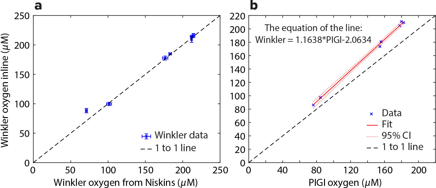
FIGURE 2. (a) Winkler data for the inline vs CTD comparison. (b) The offset between the Winkler data and the PIGI system. Error bars show standard deviation. Further, the lowest O2 sample shown in (a) was excluded from (b). > High res figure

 

We then compared the inline Winkler oxygen readings to the PIGI OO to evaluate the accuracy of the PIGI OO. This showed that the OO slightly underestimates the dissolved O₂ values measured by Winkler (Figure 2b). To correct for calibration offsets on the PIGI OO, we applied a linear regression between the Winkler data and the PIGI OO, excluding the estuary data point for the reasons stated above. This correction was then applied to the PIGI OO data during processing.

Processing of PIGI OO data to derive NCP followed the MATLAB script provided on the PIGI Zenodo repository (Figure 3a). The calculation includes temperature and salinity correction on both the O₂ and N₂ data based on measurements from the ship’s thermosalinograph. Calculating NCP estimates following Izett and Tortell (2021) was easily performed as the required auxiliary data was collected by R/V Savannah, including the barometric pressure, wind speed at 10 m, and mixed layer depth (determined by CTD casts). These standard oceanographic vessel measurements facilitate calculations of NCP from PIGI data. If shipboard data are not available, archival or reanalysis data can be used instead. Historical wind data are also required; we used data from the Savannah-Hilton Head International Airport, also from 10 m.

 

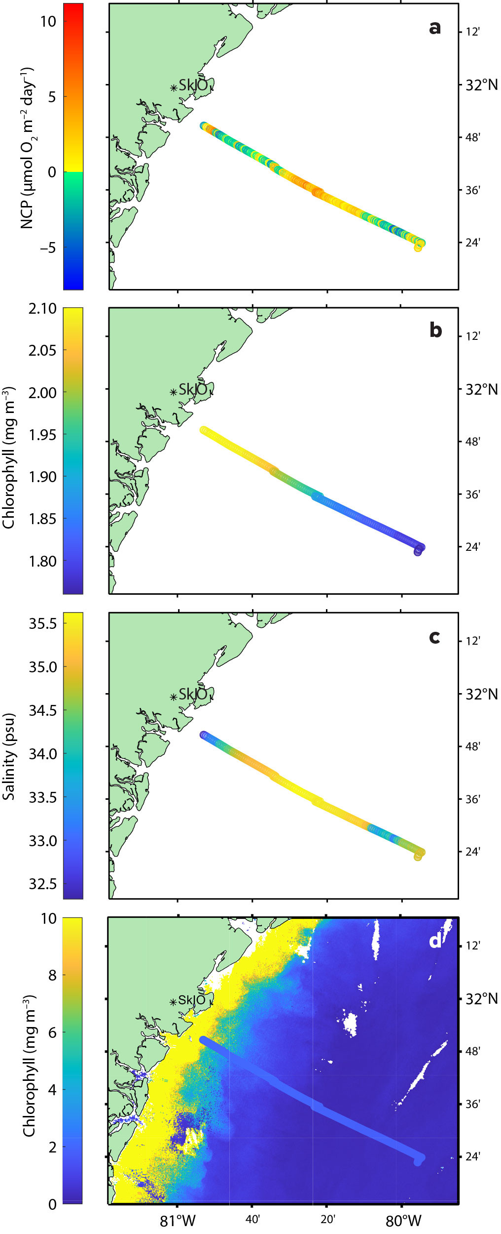
FIGURE 3. (a) Net community production from the September 24, 2023, PIGI test cruise in the South Atlantic Bight. (b) Chlorophyll a concentration from same cruise. (c) Salinity from the same cruise. (d) Chlorophyll a satellite product from Copernicus Sentinel-3 platform for September 27, 2023, with the chlorophyll from the cruise overlaid. Note the different dates and scale bars in (b) and (d). > High res figure

 

As Figure 3a shows, results from our underway analysis display negative NCP coastally, followed by increased NCP in the middle of the track, and negative NCP at the most offshore point. This coastal to offshore trend suggests that the water near the coast is affected by the estuaries, which are heterotrophic, whereas offshore waters are mostly autotrophic. Estuary heterotrophy (Hopkinson, 1985; Hopkinson et al., 1991; Signorini et al., 2005) is believed to be linked to exogenous carbon sources from surrounding salt marshes and terrestrial areas, which act as carbon sources to fuel respiration. As the tide goes out, the organic-​rich soil of the marshes is resuspended, and bacteria then break down the resuspended organic matter, consuming oxygen and leading to a negative ΔO₂/N₂ and therefore negative NCP. This low oxygen signature is exported out of the estuaries onto the SAB shelf. The secondary negative NCP aligns with a freshening of the water and the lowest chlorophyll (Figure 3b,c). The low salinity water may have been introduced to the system during heavy rains the week prior. As these rains were not accompanied by strong winds, the water may have been transported offshore as a coherent mass. This could explain the negative NCP, where the signal was exported offshore.

To better understand the PIGI system data, we compared them with chlorophyll data from September 27, 2023, collected by the Copernicus Sentinel-3 satellite (three days after the cruise due to clouds caused by the passing storm). The Copernicus data were transformed from log(chlorophyll) to chlorophyll so that they are comparable to the in situ chlorophyll data (Figure 3d). The satellite data suggest higher chlorophyll after the storm, with the same lower chlorophyll offshore as on September 24. Comparing the Copernicus chlorophyll data with the NCP data showed a mismatch that is likely due to the substantial mixing that occurred between the two measurements. At the end of the cruise track, NCP becomes negative, which is likely driven by a combination of bubble injection and entrainment of oxygen-depleted deep water that is being mixed up by the storm.

We do not show the estuarine and riverine portions of the cruise here, as they likely violate the steady-state assumptions that the PIGI system uses. These excluded data have two potential issues that can affect NCP estimates: the primary production in benthos and sedimentary waters, and the advection and horizontal mixing of waters by the tides. The marshes and estuaries in the SAB are known to have anoxic sediments that are routinely exposed at low tide (Rao et al., 2007). This means that water enriched in N₂ and reduced in O₂ is added to the water column at each low tide. Further, the SAB is mesotidal, resulting in water bodies being mixed and moved over distances up to 15 km (Menzel and US Department of Energy Environmental Sciences, 1993). This leads to dissolved gas signals becoming mixed across broad spatial scales in the region, meaning that within this shallow and tidally influenced area, the dissolved gas signal in the water column is a mixture of products from the sediment, benthic, and pelagic communities.

The PIGI system was designed for open ocean deployments. In reviewing all our results, we demonstrated that the PIGI system captures the general trends in the system and shows the expected patterns of heterotrophic estuaries giving way to autotrophic shelf waters (Hopkinson, 1985; Hopkinson et al., 1991; Signorini et al., 2005). However, the high tidal variability means that using the PIGI system in estuarine regions requires further study so that we can better understand the potential uses and limitations of this system in regions with large tidal ranges.

The technical updates to the PIGI system described have been successful. Our deployment of the PIGI system from R/V Savannah required minimal attention and maintenance. It effectively collected O₂ and N₂ data in both turbid estuarine waters and offshore waters. We recommend the PIGI system to other researchers for offshore environments, where the steady state assumptions are met based on ease of deployment, low cost, and the amount and quality of data obtained. We caution against the use of the PIGI system during storms, as bubble injection invalidates the steady state assumption.

 

Tips and Tricks

We have gained considerable knowledge that will facilitate the use of the PIGI system by a broad user group. Below, we share useful advice for others wishing to build their own systems.

The time and cost to build the PIGI system were both higher than anticipated. Building the PIGI system took seven months for us, including the time to order parts, get the PVC machined, and modify the system. We hope that this update will decrease the build time, but we would encourage potential users to realistically assess the timeline for construction based on their technical skills and access to fabrication equipment.

Build costs were higher than the estimate given in the original publication due to the cost of cutting PVC parts, choice of instruments, and inflation. Quotes from private companies for PVC machining ranged between $3,500 and $4,000, including the price of the materials. We were fortunate to be able to avoid this cost by cutting the PVC ourselves. We also chose to use the fast OO, increasing the cost of the system by $200. Inflation of ~10% has occurred for most of the materials and components on the parts list since the time of the original publication. This brings an updated cost estimate to ~$20,000 for the PIGI system, not accounting for labor and optional software licenses. In total, however, the updated costs are still significantly lower than those of a mass spectrometer, which can cost upward of $50,000.

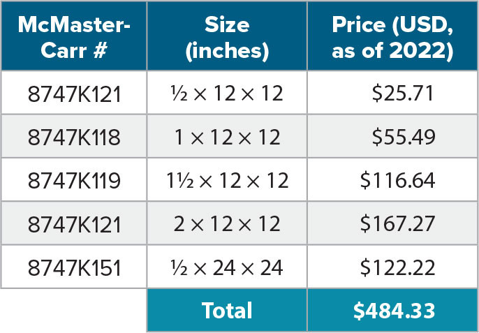
When ordering components, adjustments are required for both the OO and some minor parts. For the OO, the water deployment cable is needed and must be ordered for the PIGI system. Second, a request should be made for the OO in RS-232 (computer) mode with short output, as the PIGI system’s LabView executable needs these settings. Settings can be adjusted after the fact by configuring the sensor using a serial communication program (e.g., Realterm), following instructions in the instrument manual. With regard to ordering parts, if you plan to have LabView on the Intel NUC, you need to have at least 256 GB of space on it, as the 64 GB version is completely filled by Windows 10. We should also note that not all D-type cables have nine wires, so ensuring that those purchased have nine wires is important. Only two DB9 to USB adapters are needed. The PVC sheets needed are listed in Table 1. There is a new model for part number 5, but this does not change the layout.

 

TABLE 1. PVC sheets needed with McMaster-Carr numbers. > High res table

 

There are three tips for wiring the system. First, the RXT and DXT for the OO  are swapped in position relative to the manufacturer’s manual (Anderaa, 2017). According to the manufacturer, this is a Swedish to English translation error. The second tip is to turn the supply voltage for the flow meters down to 10 V, as the National Instruments receiver typically works between –10 and 10 V. Turning down the voltage can be done by adjusting a screw on the power source. Third, when wiring the relay to the NI DAQ, the A1 connection must go to the + a/o channel and the A2 to the ground (last terminal) of the a/o channel (see Figure 1d).

 

Conclusion

The updated PIGI system offers improved functionality and ease of use. It worked well in offshore waters, but it appears to need further testing in order to understand the complex estuarine and coastal waters of the SAB. We hope to further explore the potential uses of the system in the SAB. The improvements that we have made to the PIGI system are useful for both future and current systems and will help to make the system more accessible to the community. The PIGI system has potential for continued growth and improvement with additional support from the community. Potential future changes include removal of the de-​bubbler flow meter, changing the flow meter from the instruments so that it does not cause back pressure, removal of the pump, and the inclusion of a temperature and salinity sensor for non-ship deployments.

 

Acknowledgments

The PIGI system was purchased as part of an NSF Ocean Instrumentation Award (# 2114584). Lowin and Rivero-Calle were supported by the University of Georgia Skidaway Institute of Oceanography and the Moore Foundation (grant number #11171). The R/V Savannah cruise was part of the Semester at Skidaway undergraduate cruise.

Lowin, B., R. Izett, E. Taylor, C. Robertson, and S. Rivero-Calle 2024. Design update to “The Pressure of In-situ Gases Instrument (PIGI) for Autonomous Shipboard Measurement of Dissolved O₂ and N₂ in Surface Ocean Waters.” Oceanography 37(2):174–179, https://doi.org/10.5670/oceanog.2024.413.

• Easy-to-Read Instructions for Operating the PIGI System (Version 4.4)

Aanderaa. 2017. TD 269 Operating Manual Oxygen Optode 4330, 4831, 4835. Aanderaa Data Instruments AS, Bergen, Norway.

Boss, E., N. Haëntjens, S.G. Ackleson, B. Balch, A. Chase, G. Dall’Olmo, S. Freeman, Y. Liu, J. Loftin, W. Neary, and others. 2019. Inherent Optical Property Measurements and Protocols: Best Practices for the Collection and Processing of Ship-Based Underway Flow-Through Optical Data. IOCCG, Dartmouth, NS, Canada., https://ioccg.org/wp-content/uploads/2017/11/inline_report_15nov2017.pdf.

Craig, H., and T. Hayward. 1987. Oxygen supersaturation in the ocean: Biological versus physical contributions. Science 235(4785):199–202, https://doi.org/10.1126/science.235.4785.199.

Culberson, C. 1991. Dissolved oxygen. World Ocean Circulation Experiment: WOCE Operation Manual 3.

Cynar, H., L.W. Juranek, C.W. Mordy, D. Strausz, and S. Bell. 2022. High-resolution biological net community production in the Pacific-influenced Arctic as constrained by O₂/Ar and O₂/N₂ observations. Deep Sea Research Part II 206:105214, https://doi.org/10.1016/j.dsr2.2022.105214.

Dickson, A.G. 1994. Determination of dissolved oxygen in sea water by Winkler titration. WHP Operations and Methods.

Emerson, S. 1987. Seasonal oxygen cycles and biological new production in surface waters of the subarctic Pacific Ocean. Journal of Geophysical Research: Oceans 92(C6):6,535–6,544, https://doi.org/​10.1029/JC092iC06p06535.

Emerson, S., C. Stump, D. Wilbur, and P. Quay. 1999. Accurate measurement of O₂, N₂, and Ar gases in water and the solubility of N₂. Marine Chemistry 64(4):337–347, https://doi.org/10.1016/S0304-4203(98)00090-5.

Emerson, S. 2014. Annual net community production and the biological carbon flux in the ocean. Global Biogeochemical Cycles 28(1):14–28, https://doi.org/​10.1002/2013GB004680.

Hopkinson, C.S. 1985. Shallow-water benthic and pelagic metabolism. Marine Biology 87(1):19–32, https://doi.org/10.1007/BF00397002.

Hopkinson, C.S., R.D. Fallon, B.-O. Jansson, and J.P. Schubauer. 1991. Community metabolism and nutrient cycling at Gray’s Reef, a hard bottom habitat in the Georgia Bight. Marine Ecology Progress Series 73(2/3):105–120, https://doi.org/10.3354/meps073105.

Izett, R., and P. Tortell. 2020. The pressure of in situ gases instrument (PIGI) for autonomous shipboard measurement of dissolved O₂ and N₂ in surface ocean waters. Oceanography 33(2):156–162, https://doi.org/10.5670/oceanog.2020.214.

Izett, R.W., and P.D. Tortell. 2021. ΔO₂/N₂´ as a tracer of mixed layer net community production: Theoretical considerations and proof-of-concept. Limnology and Oceanography: Methods 19(8):497–509, https://doi.org/10.1002/lom3.10440.

Izett, R.W., L. Castro de la Guardia, M. Chanona, P.G. Myers, S. Waterman, and P.D. Tortell. 2022. Impact of vertical mixing on summertime net community production in Canadian Arctic and subarctic waters: Insights from in situ measurements and numerical simulations. Journal of Geophysical Research: Oceans 127(8):e2021JC018215, https://doi.org/10.1029/2021JC018215.

Jiang, L.-Q., W.-J. Cai, Y. Wang, J. Diaz, P.L. Yager, and X. Hu. 2010. Pelagic community respiration on the continental shelf off Georgia, USA. Biogeochemistry 98(1):101–113, https://doi.org/​10.1007/s10533-009-9379-8.

Kaiser, J., M.K. Reuer, B. Barnett, and M.L. Bender. 2005. Marine productivity estimates from continuous O₂/Ar ratio measurements by membrane inlet mass spectrometry. Geophysical Research Letters 32(19), https://doi.org/​10.1029/​2005GL023459.

Laws, E.A. 1991. Photosynthetic quotients, new production and net community production in the open ocean. Deep Sea Research Part A 38(1):143–167, https://doi.org/10.1016/0198-0149(91)90059-O.

McNeil, C., D. Katz, R. Wanninkhof, and B. Johnson. 2005. Continuous shipboard sampling of gas tension, oxygen and nitrogen. Deep Sea Research Part I 52(9):1,767–1,785, https://doi.org/10.1016/​j.dsr.2005.04.003.

Menzel, D.W., and US Department of Energy Environmental Sciences. 1993. Ocean Processes: U.S. Southeast Continental Shelf: A Summary of Research Conducted in the South Atlantic Bight Under the Auspices of the U.S. Department of Energy from 1977 to 1991. US Department of Energy, Office of Scientific and Technical Information, Oak Ridge, TN, 128 pp.

Rao, A.M.F., M.J. McCarthy, W.S. Gardner, and R.A. Jahnke. 2007. Respiration and denitrification in permeable continental shelf deposits on the South Atlantic Bight: Rates of carbon and nitrogen cycling from sediment column experiments. Continental Shelf Research 27(13):1,801–1,819, https://doi.org/​10.1016/​j.csr.2007.03.001.

Reuer, M.K., B.A. Barnett, M.L. Bender, P.G. Falkowski, and M.B. Hendricks. 2007. New estimates of Southern Ocean biological production rates from O₂/Ar ratios and the triple isotope composition of O₂. Deep Sea Research Part I 54(6):951–974, https://doi.org/10.1016/j.dsr.2007.02.007.

Shulenberger, E., and J.L. Reid. 1981. The Pacific shallow oxygen maximum, deep chlorophyll maximum, and primary productivity, reconsidered. Deep Sea Research Part A 28(9):901–919, https://doi.org/​10.1016/​0198-0149(81)90009-1.

Signorini, S.R., C.R. McClain, A. Mannino, and S. Bailey. 2005. Report on Ocean Color and Carbon Study for the South Atlantic Bight and Chesapeake Bay Regions. National Aeronautics and Space Administration, Greenbelt, Maryland, 52 pp., http://www.ccpo.odu.edu/Research/US-ECoS/sab_cb_report.pdf.

Stanley, R.H.R., J.B. Kirkpatrick, N. Cassar, B.A. Barnett, and M.L. Bender. 2010. Net community production and gross primary production rates in the western equatorial Pacific. Global Biogeochemical Cycles 24(4), https://doi.org/​10.1029/2009GB003651.

Tilstone, G.H., Y.-Y. Xie, C. Robinson, P. Serret, D.E. Raitsos, T. Powell, M. Aranguren-Gassis, E.E. Garcia-Martin, and V. Kitidis. 2015. Satellite estimates of net community production indicate predominance of net autotrophy in the Atlantic Ocean. Remote Sensing of Environment 164:254–269, https://doi.org/10.1016/j.rse.2015.03.017.

This is an open access article made available under the terms of the Creative Commons Attribution 4.0 International License (https://creativecommons.org/licenses/by/4.0/), which permits use, sharing, adaptation, distribution, and reproduction in any medium or format as long as users cite the materials appropriately, provide a link to the Creative Commons license, and indicate the changes that were made to the original content. Images, animations, videos, or other third-party material used in articles are included in the Creative Commons license unless indicated otherwise in a credit line to the material. If the material is not included in the article’s Creative Commons license, users will need to obtain permission directly from the license holder to reproduce the material.