The GEOTRACES program has greatly expanded measurements of trace elements, which serve as key nutrients, harmful contaminants, and tracers of ocean processes and past conditions. Many elements tend to associate with particulate matter, and GEOTRACES has been particularly valuable for growing our understanding of this fraction. Focusing on the micronutrient iron as an example, GEOTRACES data demonstrate that the majority of iron in the ocean is particulate. Chemically labile particulate iron, likely available for biological use, is also often more abundant than dissolved forms, particularly near continents and in the deep sea. This highlights the need to consider the particulate fraction in conceptual and numeric ocean models. Direct comparisons of particle-sampling methods highlight both the abundance of small particles (<0.45–0.8 μm), whose biogeochemical roles are still poorly known, and the difficulty in consistently capturing large, faster-sinking particles. In situ pumps with 0.8 μm filters often capture less small particulate iron than bottle-collected samples filtered onto 0.45 μm filters, but they can also capture more material near some sources. GEOTRACES datasets contain nearly sevenfold more dissolved than particulate iron measurements, and ongoing efforts to pair these measurements are needed in order to fully understand the cycles of iron and other important elements.

Collection of dissolved and particulate trace elements during the GEOTRACES GP17-OCE cruise. Photo credit: B. Twining. > High res figure

Introduction

Trace elements play many important roles in the ocean, from providing critical micronutrients to serving as signatures of unique material sources and as tracers of past processes, belying their low concentrations (Morel and Price, 2003). The GEOTRACES program was initiated to advance our understanding of the geochemistry of trace elements and their isotopes (TEIs) and to fill key knowledge gaps about the sources, sinks, and internal cycling of trace elements (Anderson, 2020). Through the hard work of many, and as a result of significant international cooperation, the GEOTRACES program has so far generated tens of thousands of intercomparable trace element measurements, underpinning basin-scale and global maps of element distributions (Schlitzer et al., 2018). These maps have enabled the identification and quantification of new sources and sinks of TEIs across ocean boundaries, as well as the development of a new appreciation for the ecological and biogeochemical impacts of trace elements.

One of the primary characteristics of trace elements is whether they exist primarily in dissolved or particulate forms. Dissolved elements generally occur as ions, which can freely participate in chemical reactions such as complexation and precipitation or binding to a phytoplankton ion transport channel. Dissolved constituents in the ocean are dominated by the major salts (e.g., Na⁺, Cl^–), which are highly soluble, occur at millimolar concentrations, and have extremely long residence times. But trace elements show a wide range of solubilities and chemical behaviors, and many of them associate readily with particles. Particulate matter often enters the ocean from continents via river run-off or aeolian dust or resuspension of shelf sediments; these are called lithogenic particles. Particulate matter can also be formed in situ through precipitation and adsorption (termed authigenic particles) and through biological growth (biogenic particles).

Particulate trace elements have unique physical and chemical behaviors that often differ fundamentally from their dissolved counterparts, driving important consequences for their residence times, sources, and sinks. Particulate phases are prone to gravitational sinking. They can adsorb or “scavenge” (Goldberg, 1954) other ions onto their surfaces and thus remove them from the dissolved phase; alternatively, they can dissolve and serve as sources of element ions. Small particles can aggregate into larger particles and be subsequently disaggregated by physical shear or biological processes. Plankton interact with particulate elements differently than with dissolved forms: a subset of taxa are able to directly consume particles via phagotrophy (Nodwell and Price, 2001), but most taxa can only access dissolved elements (Sutak et al., 2020). Like the better-​studied dissolved trace elements, the speciation of particulate TEIs can also indicate their sources and the processes affecting their transformations. For example, particulate minerals delivered via atmospheric deposition, hydrothermal vents, and sediment resuspension have unique elemental stoichiometries, as does biogenic particulate matter (Lam et al., 2012; Twining and Baines, 2013; Hawco et al., 2018; Hoffman et al., 2018).

Despite their importance, particulate elements have received far less attention than dissolved forms. One reason is practical: oceanographers usually filter sea­water to isolate the dissolved phase, and the high-efficiency cartridge filters often used are not easily opened in order to recover the particles for analysis. Particle collection therefore typically entails using thin membrane filters, which can complicate the simultaneous collection of dissolved samples without TEI contamination (Cutter et al., 2017). Particle collection onto membranes also necessitates filtering adequate volumes to observe the elements above detection limits and background concentrations in the membrane. Achieving analyte signal greater than the filter is often trivial for major elements like carbon and nitrogen that can be collected onto glass fiber filters with low background levels, but the trace (ca. 10⁶-fold lower), contamination-​prone character of most TEIs makes their measurement a challenge. Rigorously cleaned, carbon-​based membranes are usually used, and collection must be done under stringent, particle-​free, clean-​room conditions. Even then, achieving adequate analytical signals is challenging, particularly for the most contamination-​prone elements such as zinc.

The choice of filter membrane thus represents an operational definition of the particulate fraction, and the use of different filter membrane types introduces complications for comparing measurements. Polycarbonate track-etched membranes with discrete, laser-cut pores collect particles differently from so-called “depth filter” membranes that are constructed from overlapping strands of material to produce nominal equivalent pore sizes. The effective collection sizes of membranes change as the membranes become more loaded with sample, as do the flow rates. Additionally, particles may also be collected directly in the ocean via in situ pumping, or via shipboard filtration of bottle-collected water (Figure 1). These approaches subject particles to different shear and osmotic stresses, and they differ in their ability to collect larger, potentially faster-sinking particulate matter. Once collected, particles usually need to be solubilized prior to analysis, and different science groups may use different digestion schemes optimized for their own needs, complicating intercomparison between groups (Ohnemus et al., 2014). These complications have historically been a major hindrance to creating intercomparable datasets of particulate element distributions, and resolving them is one of the key advances of extensive and ongoing GEOTRACES intercalibration efforts.

 

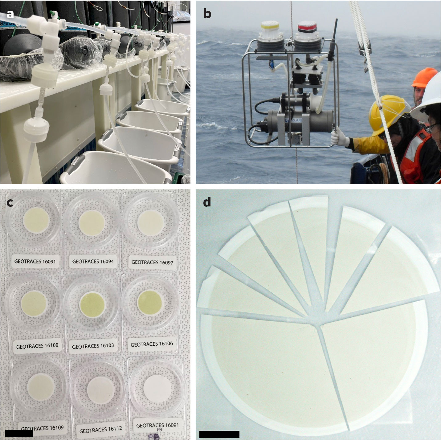
FIGURE 1. Photographs show the collection of particulate matter by (a) bottle filtration, and (b) in situ pump filtration. Particulate matter is collected onto either (c) 25 mm diameter, 0.45 μm pore-size Supor membranes for bottle filtration, or (d) 142 mm diameter, 0.8 μm pore-size Supor membranes for pump filtration. The scale bars in (c) and (d) represent 25 mm. Panel d photograph provided by Daniel Ohnemus. > High res figure

 

GEOTRACES Measurements of Particulate Trace Elements

The GEOTRACES program has created the first global dataset of intercomparable particulate trace element measurements. Recognizing the operational challenges of particulate element collection and measurement, the GEOTRACES program standardized protocols, focusing on two complementary approaches: collection of particulate matter via shipboard filtration of bottle-collected water (so called “bottle particles”; Figure 1a,c), and in situ filtration by pumps suspended in the water column (“pump particles”; Figure 1b,d). Additionally, GEOTRACES organized intercalibration exercises that employed common samples and certified reference materials to ensure that resulting analyses would be comparable (Planquette and Sherrell, 2012; Ohnemus et al., 2014). GEOTRACES has taken the additional step to periodically compile and distribute a single dataset of quality-assured measurements to promote their use by the oceanographic community. The most recent intermediate data product was released in July 2023 (IDP2021v2).

The IDP2021v2 dataset includes particulate concentrations for 17 different elements, most of them associated with multiple types of particles. Phosphorus is frequently used as a proxy for biogenic matter, and aluminum and titanium are useful proxies for lithogenic matter. Also included are the bioactive micronutrient elements (iron, manganese, cobalt, nickel, copper, zinc, cadmium), and other elements that can serve as tracers of processes (barium, chromium, molybdenum, scandium) or particle sources (lead, thorium). Each element can tell a unique story; here, I will focus on iron, the key limiting nutrient. IDP2021v1 includes particulate data from nine cruises spanning primarily the Atlantic, Pacific, and Arctic ocean basins (Figure 2b). The dataset contains 2,486 measurements of particulate iron collected via bottles at 164 different stations. In contrast, the same dataset contains nearly sevenfold more dissolved Fe measurements—​15,970 concentration data points collected on 40 cruises (Figure 2a)—​demonstrating the added challenges of collecting particulate data. Particulate iron data collected with pumps—enabling collection of the large, fast-sinking size fraction—are even harder to come by. Such data are only available from four cruises, resulting in 946 measurements from 72 stations (Figure 2c).
 

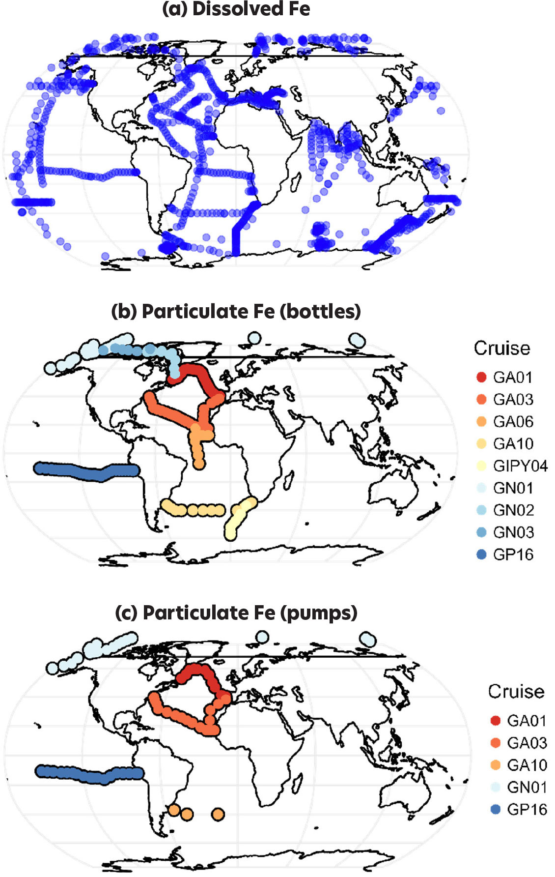
FIGURE 2. Distribution of stations for which data are available in the GEOTRACES Intermediate Data Product 2021v2. Panels show the locations of stations with data for (a) dissolved Fe, (b) bottle-collected particulate Fe, and (c) pump-collected particulate Fe. Dissolved Fe data come from 40 individual cruises. Particulate data have been collected on a much smaller number of cruises. The GEOTRACES cruise designations are indicated by symbol color. > High res figure

 

Despite the enormous effort that has gone into compiling the IDP2021v2 dataset, there remain challenges to examining all particulate data together. Unlike dissolved iron (DFe), which is represented by one parameter in IDP2021v2, there are seven different parameters for particulate iron, some of which are subsets of one another, and some of which may or may not provide equivalent information. To enable direct comparisons of dissolved and particulate data collected at the same station and depth, I calculated total particulate iron concentrations (TPFe), where necessary, and then merged to common depths for which dissolved iron data are available, when collected within 5 m of the dissolved sample.

 

Relative Concentrations of Particulate and Dissolved Iron

Though previous studies have asserted that most iron in the upper ocean is particulate (Radic et al., 2011; Gourain et al., 2019), few of them have compared paired measurements across diverse settings. This dataset provides an ideal chance to compare the two forms, and we can see that particulate and dissolved iron often show similar distributions due to transformations between them. But particulate iron is not bound by the limits of solubility and shows a greater dynamic range than dissolved iron. Focusing on two ocean basin sections—GP16 in the South Pacific and GA01 in the North Atlantic (Figure 3)—we see that continental margins are sources of both dissolved and particulate iron (Ohnemus and Lam, 2015; Lee et al., 2018; Gourain et al., 2019), as is the East Pacific Rise hydrothermal field (Resing et al., 2015; Fitzsimmons et al., 2017). The highest DFe concentrations on GP16 (31 nmol kg^–1) are observed in 110 m of water over the South American shelf, while in the core of the neutrally buoyant plume, DFe peaks at 13.7 nmol kg^–1 (Figure 3a). In contrast, TPFe reaches fivefold higher (159 nmol kg^–1) over the shelf and sixfold higher (88 nmol kg^–1) in the core of the hydrothermal plume (Figure 3b). The decoupling is even stronger in the North Atlantic, where DFe of 7.6 nmol kg^–1 was observed over the North American margin (Figure 3d), compared to 168 nmol kg^–1 TPFe (Figure 3e). Interestingly, TPFe was even higher on the European margin, registering 304 nmol kg^–1, whereas DFe peaked at 3.0 nmol kg^–1 (Gourain et al., 2019).

 

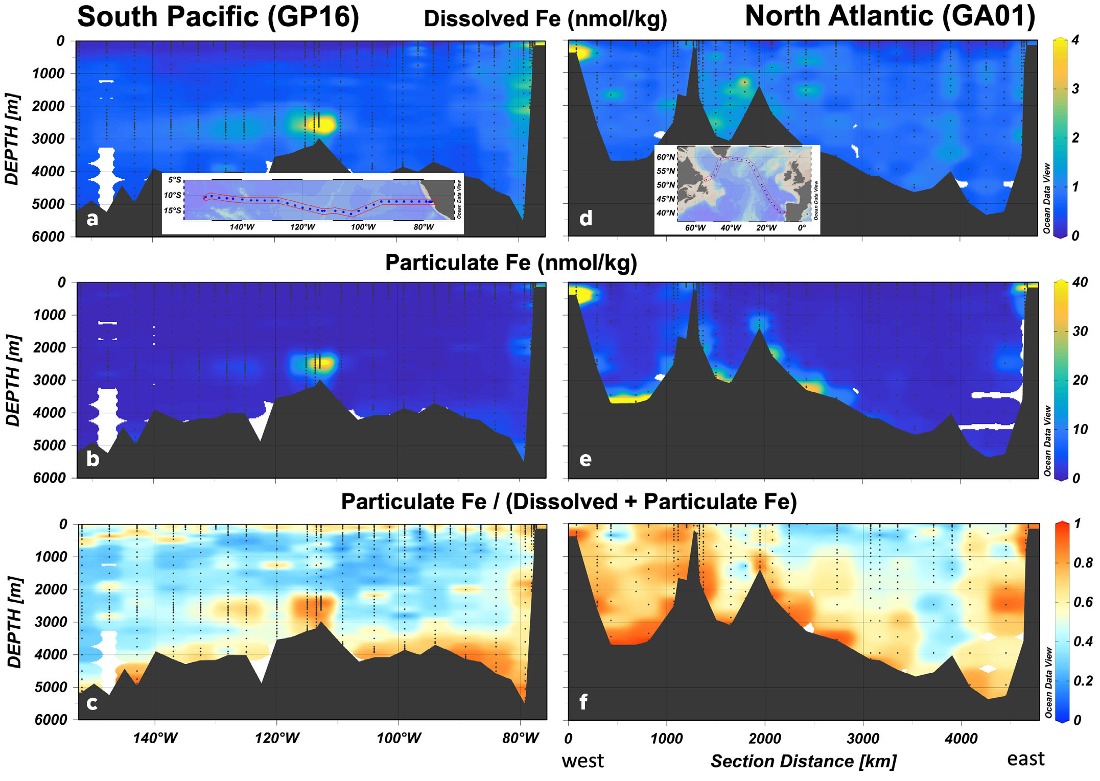
FIGURE 3. Distributions of dissolved and particulate Fe in the South Pacific (GP16 cruise) and North Atlantic (GA01 cruise). Top panels (a, d) show concentrations of dissolved Fe. Middle panels (b, e) show concentrations of total particulate Fe (>0.45 μm material, collected with bottles). Concentration color scales in a–c do not indicate the maximum concentrations measured but are optimized to show features. Bottom panels (c, f), show particulate Fe as a fraction of total (dissolved + particulate) Fe. Warm colors (yellow/orange/red) indicate particulate Fe >50% of total Fe. Cool colors (blue) indicate particulate Fe <50% of total Fe. > High res figure

 

Particulate iron shows a third source not evident in the dissolved dataset: benthic nepheloid layers. In the North Atlantic, suspended sediments near the bottom drive TPFe concentrations above 60 nmol kg^–1 (Figure 3e), while DFe is not correspondingly elevated. This may indicate the limits of iron solubility—particularly as iron ligand concentrations are not elevated near bottom (Buck et al., 2018)—or counteracting adsorption and dissolution processes. As a result of these processes, particulate iron typically exceeds dissolved iron at the ocean interfaces—​surface, margins, benthos, and vent plumes. In these settings, >85% of total iron (dissolved + particulate) is present in particulate form (Figure 3c). In the mesopelagic, TPFe is less abundant than DFe—typically 20%–30% of total Fe. Overall, particulate is a bigger component of total iron in the North Atlantic, where it is commonly more than 60% of total iron, even in the ocean interior (Figure 3f). Interestingly, despite abundant aeolian deposition, TPFe does not exceed DFe in surface waters of the Northeast Atlantic, as DFe is not drawn down as much in these waters.

These same trends can be observed when considering all of the paired particulate and dissolved iron data available in IDP2021v2. Particulate Fe shows a greater range, with concentrations varying more than 10,000-fold, from less than 0.1 to over 1,000 nmol kg^–1 (Figure 4a). In contrast, DFe varies about 100-fold, from less than 0.1 to over 10 nmol kg^–1. While clearly positively correlated, TPFe increases more rapidly than DFe, with the greatest decoupling at shallow stations where margin inputs of lithogenic particulate matter are greatest.

Overall, iron is more commonly found in particulate than dissolved form. Figure 4b shows the distribution of the particulate/dissolved Fe ratio for the 1,950 paired measurements in IDP2021v2. For each of the sample depth ranges (Shallow, Mid, Deep), particulate/dissolved ratios greater than 1 are most common. The mean and median ratios are 7.1 and 1.9, respectively. Thus, particulate Fe is typically about twice as abundant as dissolved Fe. The relative abundance of particulate Fe enables it to buffer the concentration of dissolved Fe (Milne et al., 2017). However, the standard deviation of the global particulate/dissolved ratio is 28, demonstrating the frequent decoupling of these two forms.

 

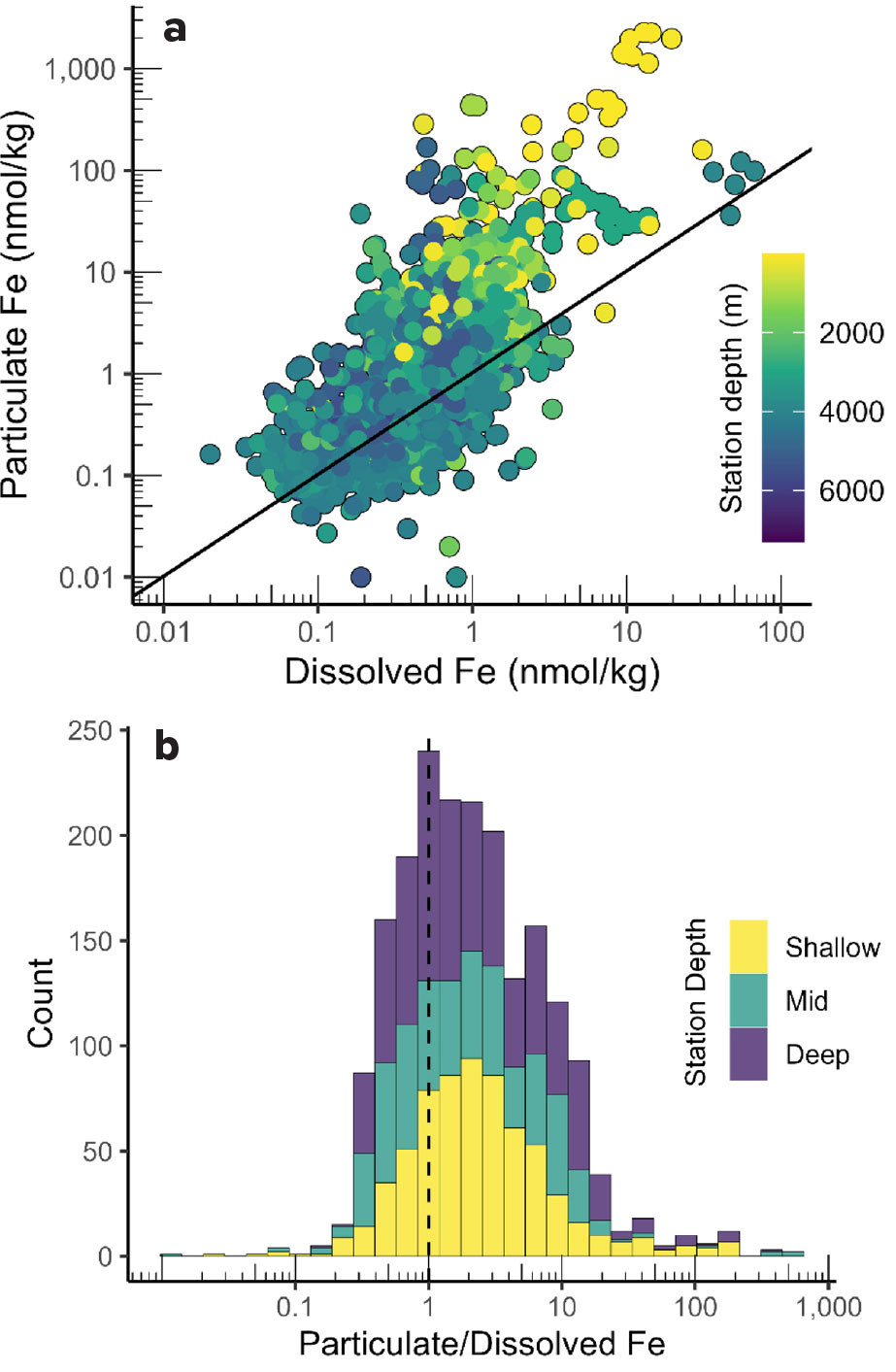
FIGURE 4. Relationship between dissolved and total particulate (>0.45 μm material, collected with bottles) Fe in the global GEOTRACES IDP2021v2 dataset. (a) Scatterplot of dissolved and particulate concentrations. Black line indicates 1:1 relationship. Symbol color indicates total water column depth at the sampling station. Note the log10 scales. (b) Histogram of particulate/​dissolved concentration ratio for all paired data in the global dataset. Bar color indicates the depth of sample collection (Shallow: <200 m; Mid: 200–1,000 m; Deep: >1,000 m). The dashed line indicates where the two fractions are equal. > High res figure

 

Contribution of Labile Particulate Iron to the Reactive Iron Pool

There is particular interest in the chemically labile forms of particulate elements such as Fe that serve as nutrients. These labile particles may contribute to the dissolved element pool in the euphotic zone and support productivity over biologically relevant timescales (Bruland et al., 2001; Chase et al., 2005; Hurst and Bruland, 2007). Several approaches have been used to measure chemical lability, including extractions with the reductant sodium dithionite (Poulton and Raiswell, 2005), mixtures of the ligand EDTA and the reductant oxalic acid (Tovar-Sanchez et al., 2003; Tang and Morel, 2006; Revels et al., 2015), and mixtures of acetic acid and the reductant hydroxylamine hydrochloride (Chester and Hughes, 1967; Tessier et al., 1979; Berger et al., 2008). The approach of Berger et al. (2008) has been adopted by several groups to measure labile particulate Fe in the GEOTRACES program, and there are four cruises for which labile particulate Fe (PFe_labile) data are available in IDP2021v2: GA03 and GA10 in the Atlantic, GP16 in the Pacific, and GN01 in the Arctic.

The labile particulate Fe data span diverse marine environments, and the contribution of PFe_labile to the reactive Fe pool (PFe_labile + DFe) varies from 0%–100% across the dataset (Figure 5a). PFe_labile shows different importance in the Pacific and the Arctic. In the Pacific, PFe_labile contributes >50% of reactive Fe in the upper ocean near the South American shelf and at the upper boundaries of the oxygen deficient zone and is otherwise mostly <40% of reactive Fe in the upper 1,000 m (Figure 5b). In contrast, most of the Arctic Ocean samples from below 200 m show PFe_labile as the dominant fraction, usually >75% of reactive Fe (Figure 5c). PFe_labile also comprises most reactive iron over the shelf; it is only in the upper 100 m of the ice-covered Arctic Ocean north of 80°N where DFe dominates, likely a result of the Fe distribution in the Transpolar Drift (Charette et al., 2020). This highlights the much greater influence of shelves—and the particles they generate (Xiang and Lam, 2020; Colombo et al., 2021, 2022)—on the Arctic interior compared to the Pacific. North Atlantic samples are limited to the upper 200 m in IDP2021v2, and they also show strong shelf inputs of labile particles (Ohnemus and Lam, 2015). Overall, the available data show the broad importance of continental shelves as sources of reactive iron, often exceeding levels of dissolved iron. Further offshore, PFe_labile is likely drawn down in concert with DFe, potentially through dissolution and direct uptake, as it buffers the dissolved pool (Milne et al., 2017), as well as through scavenging of labile Fe oxyhydroxides onto more refractory oxides as particles change in chemistry, size, and age during transit (Fitzsimmons et al., 2017; Hoffman et al., 2018).

 

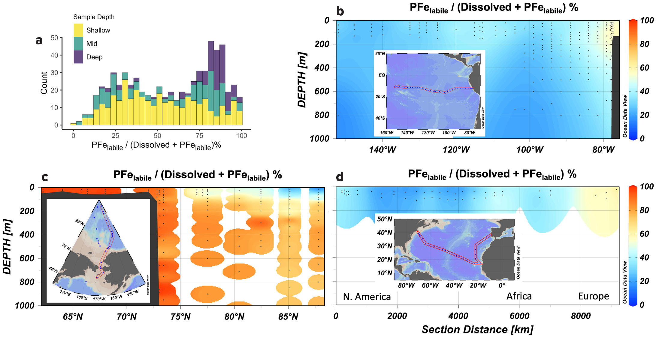
FIGURE 5. Relationships between dissolved and labile particulate Fe (PFelabile). (a) Histogram of PFelabile as a percent of reactive (Dissolved + PFelabile) Fe. Bar color indicates the depth of sample collection (Shallow: <200 m; Mid: 200–1,000 m; Deep: >1,000 m). (b) Section of PFelabile as percent of reactive Fe in the South Pacific (GP16 cruise). Warm colors (yellow/orange/red) indicate PFelabile >50% of reactive Fe. Cool colors (blue) indicate PFelabile <50% of reactive Fe. Data are only available for the upper 1,000 m. (c) Equivalent section for the eastern leg of the GN01 Arctic cruise. Data are only shown for the upper 1,000 m. (d) Equivalent section for the GA03 North Atlantic Cruise. Data are only available for the upper 150 m. > High res figure

 

Collection of Particulate Matter by Bottles and Pumps

GEOTRACES investigators have used both sampling bottles and in situ pumps to collect particulate matter for TEI analysis, and comparisons of these measurements can provide additional information about particulate trace elements. In situ pumps can achieve higher sample loading and larger absolute sample masses, which enable measurements of trace element stable isotopes and the rarest elements. Additionally, parallel filtration onto different membranes via pumps enables simultaneous measurements of organic and inorganic carbon, along with opal and trace element fractions. Pump-based particle datasets from the Atlantic (Lam et al., 2015a; Ohnemus and Lam, 2015), Pacific (Lam et al., 2018; Lee et al., 2018), and Arctic Ocean (Xiang and Lam, 2020) are included in IDP2021v2. These efforts have generated paired measurements of particulate organic matter (POM), particulate inorganic carbon (PIC), opal, lithogenic matter, Fe oxides, and Mn oxides that comprise the major components of particulate matter in the ocean. Distributions of these components reflect their known sources: creation of POM in the euphotic zone, synthesis of opal by mostly coastal diatoms, lithogenics from continents and aeolian dust, and in situ precipitation of Mn and Fe oxides.

The larger volumes filtered with in situ pumps are also likely to better sample larger (>51 μm), rarer particulate matter, providing information on two size fractions and the cycling between them. Thorium isotope data indicate active aggregation and disaggregation processes are at play, resulting in continual exchange between large and small particles (Lerner et al., 2016). In some instances, large particles have been shown to be a key component of particulate matter. In the North Atlantic, it is common for more than half of particulate iron to be >51 μm in the upper 200 m (Ohnemus and Lam, 2015). In the Pacific, iron is more abundant in large particles in the euphotic zone and near the bottom, but across the basin it is generally sourced from small particles (Lee et al., 2018). In the Arctic, iron in large particles is mostly restricted to the bottom of the water column (Xiang and Lam, 2020).

The collection of particulate matter with both bottles and pumps on several GEOTRACES cruises provides an opportunity to learn more about particulate trace element composition from comparison of these measurements. Here, I will focus on two GEOTRACES sections, one in the South Pacific (cruise GP16) and the other in the Arctic (cruise GN01). Together, they provide an opportunity to expand on a previous comparison that was based on a handful of mostly upper water column profiles from the North Atlantic (Twining et al., 2015). Pump-collected particulate iron concentrations (0.8–51 μm small + >51 μm large size fractions; “pump Fe”) for the Pacific and Arctic are shown in Figure 6, for comparison with the bottle-collected particulate iron concentrations (>0.45 μm; “bottle Fe”) shown in Figure 3. The two sampling approaches produce similar particulate iron distributions (Figure 6a,d), with the South American margin and East Pacific Rise clear sources of iron to the South Pacific, and the Bering Sea and Chukchi shelves strong sources to the Arctic. Pump and bottle iron measurements collected within 5 m of each other are directly compared in Figure 6b and 6e. In the Pacific, pumps collected more particulate iron most commonly at shallow stations and near the surface, and this is also evident on the Arctic shelf. In the mid water column and offshore, it is more common for bottle samples to show higher particulate iron.

 

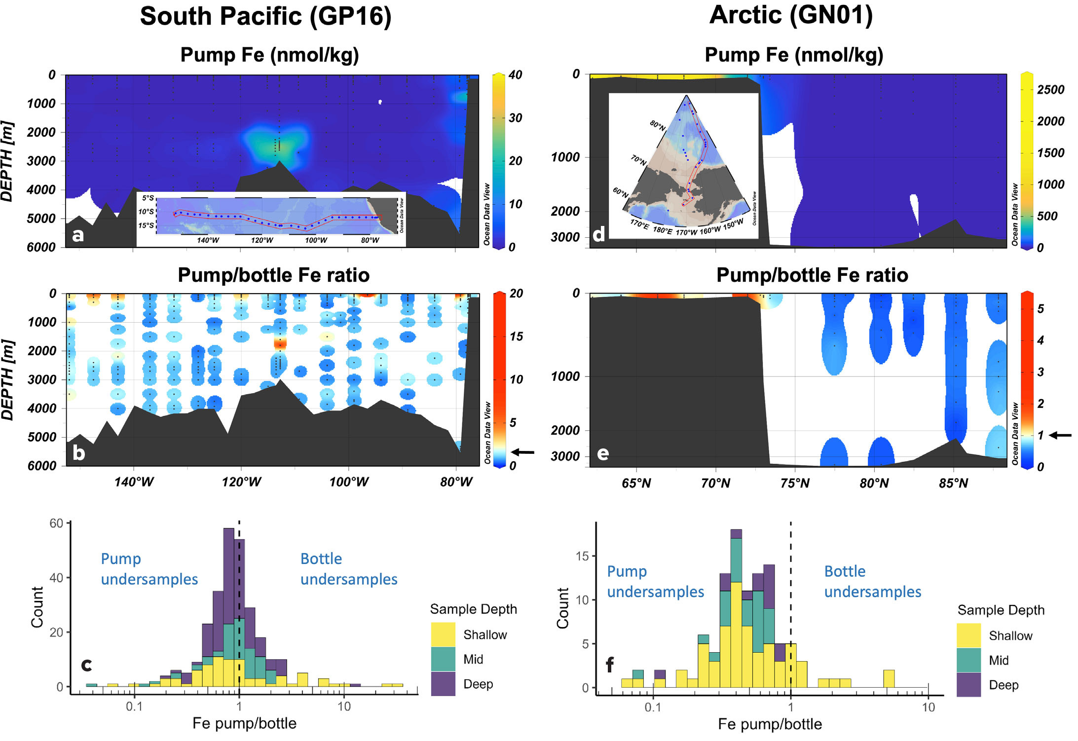
FIGURE 6. Distributions of particulate Fe (>0.8 μm) collected in the South Pacific (GP16) and Arctic (GN01) with in situ pumps. Top panels (a, d) show concentrations. Middle panels (b, e) show the ratio of pump-collected Fe (sum of small and large size fraction) to bottle-collected Fe for samples collected at the same station within 5 m of each other. Warm colors (yellow/orange/red) indicate pump Fe greater than bottle Fe. Cool colors (blue) indicate pump Fe less than bottle Fe. Arrow indicates unity on the color scale. Bottom panels (c, f) show histograms of pump/bottle Fe ratio for each section. There are 281 paired points of comparison for the GP16 dataset and only 105 points of comparison in the GN01 dataset, as many of the deeper samples were offset by more than 5 m. Bar color indicates the depth of sample collection (Shallow: <200 m; Mid: 200–1,000 m; Deep: >1,000 m). The dashed line indicates where the two fractions are equal. > High res figure

 

Combining all 281 paired particulate Fe measurements in the South Pacific, several trends appear (Figure 6c). The median ratio of pump/bottle Fe was 0.87 ± 2.7 (1 std dev), highlighting substantial variability in the paired comparisons. The greatest discrepancies between the sampling approaches were seen in shallow waters, which are characterized by greater particle heterogeneity and larger, faster-sinking, short-lived particles prone to under-sampling by bottle filtrations. Most of the measurements on the section were from depths >1,000 m, where bottles tend to collect more particulate Fe than pumps. This is notably evident in the neutrally buoyant hydrothermal plume west of 113°W. Micro-analytical images of plume particles revealed Fe(III) oxyhydroxide particles >2 μm associated with organic carbon matrices (Fitzsimmons et al., 2017), which should be collected by both bottles and pumps. However, colloidal Fe particles <0.2 μm are abundant in the deep ocean and important contributors to the size spectrum of Fe (Fitzsimmons et al., 2015). The 0.45 μm and 0.8 μm filters used in bottle and pump sampling, respectively, will likely have different capture efficiencies for these small particles, explaining the higher absolute deep particulate iron concentrations. Interestingly, the pump-bottle difference was weaker at mesopelagic depths (Figure 6c “Mid” depth bin: 200–1,000 m; median=1.01), where colloidal iron is relatively less abundant (Fitzsimmons et al., 2015). Thus, pump-bottle differences in the Pacific demonstrate differences in sampling efficiency for both rarer large particles and abundant very small particles.

The GN01 Arctic section also has full-depth particulate measurements from pumps and bottles, and these again show similar iron distributions (Figure 6d,e). There are fewer paired measurements collected within 5 m of each other due the heightened operational challenges of sample collection in the often ice-​covered Arctic. The 105 paired comparisons show a greater offset than in the Pacific, with median pump/bottle particulate iron of 0.47, and all mid-depth and deep pump/bottle Fe ratio comparisons less than 1 (Figure 6f). All instances of bottle iron under-sampling pump iron occurred in shallow waters, where again large, potentially faster-sinking particles can be missed by bottle sampling. This offset is not caused by analytical differences, as all research groups reported ca. 100% iron recoveries for multiple certified reference materials. Further, pump and bottle research groups exchanged both pump-collected and bottle-collected replicate filters for parallel digestion and analysis, and these comparisons did not show consistent offsets. Instead, the different particulate iron concentrations likely result from the different filter pore sizes used. Supporting this, bottle iron concentrations measured by European colleagues at a “cross-over station” at 88°N within a few months of the US occupation produced very similar results to US bottle Fe (Hélène Planquette, French National Centre for Scientific Research, unpublished data). It thus appears that a greater proportion of particulate iron in the Arctic falls within a 0.45–0.8 μm fraction that is differentially sampled by pumps and bottles.

Differences in bottle- and pump-​sampled particulate iron can be further discerned by looking at individual station profiles. Figure 7 shows particulate iron profiles from two stations each in the Pacific and the Arctic. Pacific Station 1, offshore from the South American shelf, shows good agreement between pump and bottle iron except at shelf depths: pumps over-collected bottles by an average of 6.6-fold in the upper 500 m (Figure 7c). Far offshore to the west at Station 25, bottle and pump iron concentrations agree in the upper 2,000 m, but bottles collected on average 50% more particulate iron in the hydrothermal plume (Figure 7b). In the Arctic, Station 57 north of the Chukchi shelf shows reasonable agreement between bottle and pump particulate iron throughout the water column except in the upper 200 m, where bottles collected 2- to 13-fold higher particulate iron (Figure 7e). This indicates that iron oxyhydroxides formed over the Chukchi shelf contain a significant fraction of 0.45–0.8 μm particles and appear to be even more abundant than noted previously (Xiang and Lam, 2020). Farther north into the Arctic basin, Station 48 (80.4°N) shows more divergent bottle and pump iron concentrations: bottle iron is consistently 2–3 fold higher than pump iron throughout the water column, suggesting that small shelf-sourced particles may comprise a significant part of particulate iron in the Arctic basin interior.

 

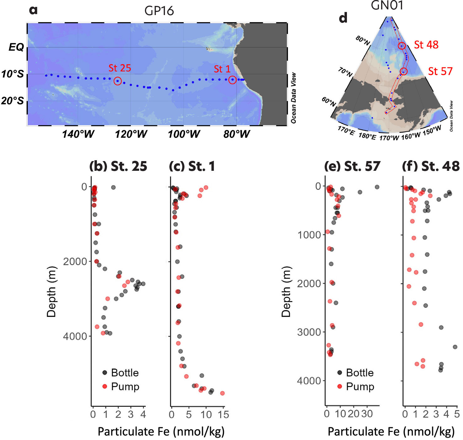
FIGURE 7. Comparisons of particulate Fe collected with bottles or in situ pumps at four stations. Left panels show data for stations 25 (b; 125°W) and 1 (c; 79.2°W) in the Pacific. Right panels show data for stations 57 (e; 73.4°N) and 48 (f; 80.4°N) in the Arctic. Black symbols indicate bottle-collected particles (>0.45 μm), and red symbols indicate pump-collected particles (>0.8 μm). > High res figure

 

Within the context of all paired bottle and pump data available in IDP2021v2, spanning three ocean basins, pumps appear to collect about 20% less particulate iron, on average, with significant variability (median pump/​bottle Fe = 0.80 ± 2.1 standard deviation). Pumps collect at higher flow rates through larger pore-size membranes than bottles, likely driving this overall bias. Due to their larger sampling volumes, however, pumps are more likely to capture rare large particles and can provide distributable subsamples for multiple analyses.

 

Conclusions and Predictions for the Next Decade of Progress

The GEOTRACES program has significantly expanded understanding of the role of particulate matter in the cycling of trace elements in the global ocean. Particles exert important controls on dissolved element concentrations, and thus must be tracked in parallel with the dissolved fraction. Doing so highlights particular locations, such as nearshore and near-bottom environments, where particles are particularly important. Indeed, particles are more often than not the predominant physical form of iron in the ocean. Notably, the Arctic basin—​surrounded by continental shelves—​harbors elevated particulate iron concentrations. Chemically labile particles should be recognized as often making significant contributions to the reactive, actively cycled iron pool. Additional efforts to characterize the bioavailability of labile particulate matter would also be valuable. Particulate matter is heterogeneous and dynamic and not easy to sample consistently. Through comparisons of paired data from bottles and pumps, we see the elevated importance of sub​-micron particles in a hydrothermal plume, as well as in the Arctic Ocean. It will be exciting to dive into new data from meridional sections of the North and South Pacific as they become available in the coming years.

Understanding of trace element cycling by particulate matter will be further advanced by coupling “bulk” measurements of particulate element concentrations via inductively coupled plasma mass spectrometry with micro-focused and particle-specific element measurements. Synchrotron radiation is particularly adept at providing information on distributions of elements between various particle types (Twining et al., 2008; von der Heyden et al., 2012; Marcus and Lam, 2014; Lam et al., 2015b), as well as characterizing chemical speciation (Toner et al., 2009; Ingall et al., 2013; Hoffman et al., 2018). The use of smaller pore-size filters to further distinguish colloidal matter is also shedding light on the complex cycling of sub-​micron trace elements (Roshan and Wu, 2018; Jensen et al., 2021). Paired measurements can help to delineate lithogenic, authigenic, and biogenic fractions of particulate matter (Sofen et al., 2023), as well as multivariate statistical approaches that leverage the dense data coverage provided by GEOTRACES sections (Ohnemus et al., 2019).

Additionally, we must measure transformations between particulate and dissolved forms of trace elements. Particulate matter is both a common reservoir and a source for dissolved elements, as well as one of the most important sinks for dissolved elements (via biological uptake and abiotic scavenging). We need to quantify and characterize these processes in order to advance our understanding of controls on trace elements and their subsequent implications for key ocean processes. Stable- and radio-isotopes are key tools in this effort (Black et al., 2018; John et al., 2018; Ellwood et al., 2020; Hawco et al., 2022), as are incubations (Hurst and Bruland, 2007; Burns et al., 2023), process studies (Boyd et al., 2005, 2012), and GEOTRACES-compliant time series (Tagliabue et al., 2023).

 

Acknowledgments

This work was funded by grants OCE-2023237 and OCE-2049272 from the US National Science Foundation. Assistance with data processing and visualization was provided by Jarret Mayo and Laura Sofen. This work was enabled by the hard work of many in the GEOTRACES program who lead and support the ocean cruises required to collect these data, as well as the large and collegial community of scientists who share methods, best practices, wisdom, advice, and data reviewing efforts to ensure the best possible science is done. The paper was improved by comments from Daniel Ohnemus and an anonymous reviewer.The international GEOTRACES program is possible in part thanks to the support from the US National Science Foundation (Grant OCE-2140395) to the Scientific Committee on Oceanic Research (SCOR).

Twining, B.S. 2024. An ocean of particles: Characterization of particulate trace elements by the GEOTRACES program. Oceanography 37(2):120–130, https://doi.org/10.5670/oceanog.2024.407.

Anderson, R.F. 2020. GEOTRACES: Accelerating research on the marine biogeochemical cycles of trace elements and their isotopes. Annual Review of Marine Science 12:49–85, https://doi.org/10.1146/annurev-marine-010318-095123.

Berger, C.J.M., S.M. Lippiatt, M.G. Lawrence, and K.W. Bruland. 2008. Application of a chemical leach technique for estimating labile particulate aluminum, iron, and manganese in the Columbia River plume and coastal waters off Oregon and Washington. Journal of Geophysical Research: Oceans 113(2), https://doi.org/​10.1029/​2007JC004703.

Black, E.E., K.O. Buesseler, S.M. Pike, and P.J. Lam. 2018. ²³⁴Th as a tracer of particulate export and remineralization in the southeastern tropical Pacific. Marine Chemistry 201:35–50, https://doi.org/​10.1016/j.marchem.2017.06.009.

Boyd, P.W., C.S. Law, D.A. Hutchins, E.R. Abraham, P.L. Croot, M. Ellwood, R.D. Frew, M. Hadfield, J. Hall, S. Handy, and others. 2005. FeCycle: Attempting an iron biogeochemical budget from a mesoscale SF6 tracer experiment in unperturbed low iron waters. Global Biogeochemical Cycles 19(4), https://doi.org/​10.1029/​2005GB002494.

Boyd, P.W., R. Strzepek, S. Chiswell, H. Chang, J.M. DeBruyn, M. Ellwood, S. Keenan, A.L. King, E.W. Maas, S. Nodder, and others. 2012. Microbial control of diatom bloom dynamics in the open ocean. Geophysical Research Letters 39(18), https://doi.org/10.1029/2012GL053448.

Bruland, K.W., E.L. Rue, and G.J. Smith. 2001. Iron and macronutrients in California coastal upwelling regimes: Implications for diatom blooms. Limnology and Oceanography 46:1,661–1,674, https://doi.org/​10.4319/lo.2001.46.7.1661.

Buck, K.N., P.N. Sedwick, B. Sohst, and C.A. Carlson. 2018. Organic complexation of iron in the eastern tropical South Pacific: Results from US GEOTRACES Eastern Pacific Zonal Transect (GEOTRACES cruise GP16). Marine Chemistry 201:229–241, https://doi.org/​10.1016/j.marchem.2017.11.007.

Burns, S.M., R.M. Bundy, W. Abbott, Z. Abdala, A.R. Sterling, P.D. Chappell, B.D. Jenkins, and K.N. Buck. 2023. Interactions of bioactive trace metals in shipboard Southern Ocean incubation experiments. Limnology and Oceanography 68:525–543, https://doi.org/​10.1002/lno.12290.

Charette, M.A., L.E. Kipp, L.T. Jensen, J.S. Dabrowski, L.M. Whitmore, J.N. Fitzsimmons, T. Williford, A. Ulfsbo, E. Jones, R.M. Bundy, and others. 2020. The Transpolar Drift as a source of riverine and shelf-derived trace elements to the central Arctic Ocean. Journal of Geophysical Research: Oceans 125:e2019JC015920, https://doi.org/​10.1029/​2019JC015920.

Chase, Z., B. Hales, T. Cowles, R. Schwartz, and A. van Geen. 2005. Distribution and variability of iron input to Oregon coastal waters during the upwelling season. Journal of Geophysical Research: Oceans 110(C10), https://doi.org/​10.1029/2004JC002590.

Chester, R., and M.J. Hughes. 1967. A chemical technique for the separation of ferro-​manganese minerals, carbonate minerals and adsorbed trace elements from pelagic sediments. Chemical Geology 2:249–262, https://doi.org/​10.1016/0009-2541(67)90025-3.

Colombo, M., B. Rogalla, J. Li, S.E. Allen, K.J. Orians, and M.T. Maldonado. 2021. Canadian Arctic Archipelago shelf-ocean interactions: A major iron source to Pacific derived waters transiting to the Atlantic. Global Biogeochemical Cycles 35:e2021GB007058, https://doi.org/​10.1029/​2021GB007058.

Colombo, M., J. Li, B. Rogalla, S.E. Allen, and M.T. Maldonado. 2022. Particulate trace element distributions along the Canadian Arctic GEOTRACES section: Shelf-water interactions, advective transport and contrasting biological production. Geochimica et Cosmochima Acta 323:183–201, https://doi.org/10.1016/​j.gca.2022.02.013.

Cutter, G.A., K. Casciotti, P. Croot, W. Geibert, L.-E. Heimburger, M. Lohan, H. Planquette, and T. van der Flierdt, eds. 2017. Sampling and sample-handling protocols for GEOTRACES cruises (v. 3.0), 178 pp., https://geotracesold.sedoo.fr/images/Cookbook.pdf.

Ellwood, M.J., R.F. Strzepek, P.G. Strutton, T.W. Trull, M. Fourquez, and P.W. Boyd. 2020. Distinct iron cycling in a Southern Ocean eddy. Nature Communications 11:825, https://doi.org/10.1038/s41467-020-14464-0.

Fitzsimmons, J.N., G.G. Carrasco, J. Wu, S. Roshan N. Hatta, C.I. Measures, T.M. Conway, S.G. John, and E.A. Boyle. 2015. Partitioning of dissolved iron and iron isotopes into soluble and colloidal phases along the GA03 GEOTRACES North Atlantic Transect. Deep Sea Research Part II 116:130–151, https://doi.org/10.1016/j.dsr2.2014.11.014.

Fitzsimmons, J.N., S.G. John, C.M. Marsay, C.L. Hoffman, S.L. Nicholas, B.M. Toner, C.R. German, and R.M. Sherrell. 2017. Iron persistence in a distal hydrothermal plume supported by dissolved-particulate exchange. Nature Geoscience 10:195–201, https://doi.org/10.1038/ngeo2900.

Goldberg, E.D. 1954. Marine geochemistry: Part 1. Chemicals of the sea. Journal of Geology 62:249–265, https://doi.org/​10.1086/​626161.

Gourain, A., H. Planquette, M. Cheize, N. Lemaitre, J.-L. Menzel Barraqueta, R. Shelley, P. Lherminier, and G. Sarthou. 2019. Inputs and processes affecting the distribution of particulate iron in the North Atlantic along the GEOVIDE (GEOTRACES GA01) section. Biogeosciences 16:1,563–1,582, https://doi.org/​10.5194/bg-16-1563-2019.

Hawco, N.J., P.J. Lam, J.-M. Lee, D.C. Ohnemus, A.E. Noble, N.J. Wyatt, M.C. Lohan, and M.A. Saito. 2018. Cobalt scavenging in the mesopelagic ocean and its influence on global mass balance: Synthesizing water column and sedimentary fluxes. Marine Chemistry 201:151–166, https://doi.org/​10.1016/j.marchem.2017.09.001.

Hawco, N.J., S.-C. Yang, P. Pinedo-González, E.E. Black, J. Kenyon, S. Ferrón, X. Bian, and S.G. John. 2022. Recycling of dissolved iron in the North Pacific Subtropical Gyre. Limnology and Oceanography 67:2,448–2,465, https://doi.org/​10.1002/​lno.12212.

Hoffman, C.L., S.L. Nicholas, D.C. Ohnemus, J.N. Fitzsimmons, R.M. Sherrell, C.R. German, M.I. Heller, J.-M. Lee, P.J. Lam, and B.M. Toner. 2018. Near-field iron and carbon chemistry of non-buoyant hydrothermal plume particles, Southern East Pacific Rise 15°S. Marine Chemistry 201:183–197, https://doi.org/10.1016/j.marchem.2018.01.011.

Hurst, M.P., and K.W. Bruland. 2007. An investigation into the exchange of iron and zinc between soluble, colloidal, and particulate size-fractions in shelf waters using low-abundance isotopes as tracers in shipboard incubation experiments. Marine Chemistry 103:211–226, https://doi.org/10.1016/​j.marchem.2006.07.001.

Ingall, E.D., J.M. Diaz, A.F. Longo, M. Oakes, L. Finney, S. Vogt, B. Lai, P.L. Yager, B.S. Twining, and J.A. Brandes. 2013. Role of biogenic silica in the removal of iron from the Antarctic seas. Nature Communications 4:1981, https://doi.org/10.1038/ncomms2981.

Jensen, L.T., N.T. Lanning, C.M. Marsay, C.S. Buck, A.M. Aguilar-Islas, R. Rember, W.M. Landing, R.M. Sherrell, and J.N. Fitzsimmons. 2021. Biogeochemical cycling of colloidal trace metals in the Arctic cryosphere. Journal of Geophysical Research: Oceans 126:e2021JC017394, https://doi.org/​10.1029/​2021JC017394.

John, S.G., J. Helgoe, E. Townsend, T. Weber, T. DeVries, A. Tagliabue, K. Moore, P. Lam, C.M. Morsay, and C. Till. 2018. Biogeochemical cycling of Fe and Fe stable isotopes in the Eastern Tropical South Pacific. Marine Chemistry 201:66–76, https://doi.org/10.1016/​j.marchem.2017.06.003.

Lam, P.J., D.C. Ohnemus, and M.A. Marcus. 2012. The speciation of marine particulate iron adjacent to active and passive continental margins. Geochimica et Cosmochima Acta 80:108–124, https://doi.org/10.1016/j.gca.2011.11.044.

Lam, P.J., D.C. Ohnemus, and M.E. Auro. 2015a. Size-fractionated major particle composition and concentrations from the US GEOTRACES North Atlantic Zonal Transect. Deep Sea Research Part II 116:303–320, https://doi.org/10.1016/​j.dsr2.2014.11.020.

Lam, P.J., B.S. Twining, C. Jeandel, A. Roychoudhury, J.A. Resing, P.H. Santschi, and R.F. Anderson. 2015b. Methods for analyzing the concentration and speciation of major and trace elements in marine particles. Progress in Oceanography 133:23–42, https://doi.org/​10.1016/​j.pocean.2015.01.005.

Lam, P.J., J.-M. Lee, M.I. Heller, S. Mehic, Y. Xiang, and N.R. Bates. 2018. Size-fractionated distributions of suspended particle concentration and major phase composition from the U.S. GEOTRACES Eastern Pacific Zonal Transect (GP16). Marine Chemistry 201:90–107, https://doi.org/10.1016/​j.marchem.2017.08.013.

Lee, J.-M., M.I. Heller, and P.J. Lam. 2018. Size distribution of particulate trace elements in the U.S. GEOTRACES Eastern Pacific Zonal Transect (GP16). Marine Chemistry 201:108–123, https://doi.org/​10.1016/j.marchem.2017.09.006.

Lerner, P., O. Marchal, P.J. Lam, R.F. Anderson, K. Buesseler, M.A. Charette, R.L. Edwards, C.T. Hayes, K.-F. Huang, Y. Lu, and others. 2016. Testing models of thorium and particle cycling in the ocean using data from station GT11-22 of the U.S. GEOTRACES North Atlantic section. Deep Sea Research Part I 113:57–79, https://doi.org/10.1016/​j.dsr.2016.03.008.

Marcus, M.A., and P.J. Lam. 2014. Visualising Fe speciation diversity in ocean particulate samples by micro X-ray absorption near-edge spectroscopy. Environmental Chemistry 11:10–17, https://doi.org/​10.1071/EN13075.

Milne, A., C. Schlosser, B.D. Wake, E.P. Achterberg, R. Chance, A.R. Baker, A. Forryan, and M.C. Lohan. 2017. Particulate phases are key in controlling dissolved iron concentrations in the (sub)tropical North Atlantic. Geophysical Research Letters 44:2,377–2,387, https://doi.org/​10.1002/​2016GL072314.

Morel, F.M.M., and N.M. Price. 2003. The biogeochemical cycles of trace metals in the oceans. Science 300(5621):944–947, https://doi.org/10.1126/science.1083545.

Nodwell, L.M., and N.M. Price. 2001. Direct use of inorganic colloidal iron by marine mixotrophic phytoplankton. Limnology and Oceanography 46:765–777, https://doi.org/10.4319/lo.2001.46.4.0765.

Ohnemus, D.C., M.E. Auro, R.M. Sherrell, M. Lagerström, P.L. Morton, B.S. Twining, S. Rauschenberg, and P.J. Lam. 2014. Laboratory intercomparison of marine particulate digestions including Piranha: A novel chemical method for dissolution of polyethersulfone filters. Limnology and Oceanography Methods 12(8):530–547, https://doi.org/​10.4319/lom.2014.12.530.

Ohnemus, D.C., and P.J. Lam. 2015. Cycling of lithogenic marine particles in the US GEOTRACES North Atlantic Transect. Deep Sea Research Part II 116:282–302, https://doi.org/10.1016/​j.dsr2.2014.11.019.

Ohnemus, D.C., R. Torrie, and B.S. Twining. 2019. Exposing the distributions and elemental associations of scavenged particulate phases in the ocean using basin-scale multi-element data sets. Global Biogeochemical Cycles 33(6):725–748, https://doi.org/​10.1029/​2018GB006145.

Planquette, H., and R.M. Sherrell. 2012. Sampling for particulate trace metal determination using water sampling bottles: Methodology and comparison to in situ pumps. Limnology and Oceanography Methods 10:367–388, https://doi.org/10.4319/lom.2012.10.367.

Poulton, S.W., and R. Raiswell. 2005. Chemical and physical characteristics of iron oxides in riverine and glacial meltwater sediments. Chemical Geology 218:203–221, https://doi.org/10.1016/​j.chemgeo.2005.01.007.

Radic, A., F. Lacan, and J.W. Murray. 2011. Iron isotopes in the seawater of the equatorial Pacific Ocean: New constraints for the oceanic iron cycle. Earth and Planetary Science Letters 306:1–10, https://doi.org/10.1016/j.epsl.2011.03.015.

Resing, J.A., P.N. Sedwick, C.R. German, W.J. Jenkins, J.W. Moffett, B.M. Sohst, and A. Tagliabue. 2015. Basin-scale transport of hydrothermal dissolved metals across the South Pacific Ocean. Nature 523:200–203, https://doi.org/10.1038/nature14577.

Revels, B.N., D.C. Ohnemus, P.J. Lam, T.M. Conway, and S.G. John. 2015. The isotopic signature and distribution of particulate iron in the North Atlantic Ocean. Deep Sea Research Part II 116:321–331, https://doi.org/10.1016/j.dsr2.2014.12.004.

Roshan, S., and J. Wu. 2018. Dissolved and colloidal copper in the tropical South Pacific. Geochimica et Cosmochima Acta 233:81–94, https://doi.org/​10.1016/j.gca.2018.05.008.

Schlitzer, R., R.F. Anderson, E.M. Dodas, M. Lohan, W. Geibert, A. Tagliabue, A. Bowie, C. Jeandel, M.T. Maldonado, W.M. Landing, and others. 2018. The GEOTRACES Intermediate Data Product 2017. Chemical Geology 493, https://doi.org/10.1016/​j.chemgeo.2018.05.040.

Sofen, L.E., O.A. Antipova, K.N. Buck, S. Caprara, L. Chacho, R.J. Johnson, G. Kim, P. Morton, D.C. Ohnemus, S. Rauschenberg, and others. 2023. Authigenic iron is a significant component of oceanic particulate iron inventories. Global Biogeochemical Cycles 37(12):e2023GB007837, https://doi.org/10.1029/2023GB007837.

Sutak, R., J.M. Camadro, and E. Lesuisse. 2020. Iron uptake mechanisms in marine phytoplankton. Frontiers in Microbiology 11, https://doi.org/10.3389/fmicb.2020.566691.

Tagliabue, A., K.N. Buck, L.E. Sofen, B.S. Twining, O. Aumont, P.W. Boyd, S. Caprara, W.B. Homoky, R. Johnson, D. König, and others. 2023. Authigenic mineral phases as a driver of the upper-ocean iron cycle. Nature 620:104–109, https://doi.org/10.1038/s41586-023-06210-5.

Tang, D.G., and F.M.M. Morel. 2006. Distinguishing between cellular and Fe-oxide-associated trace elements in phytoplankton. Marine Chemistry 98:18–30, https://doi.org/10.1016/​j.marchem.2005.06.003.

Tessier, A., P.G.C. Campbell, and M. Bisson. 1979. Sequential extraction procedure for the speciation of particulate trace metals. Analytical Chemistry 51:844–851, https://doi.org/10.1021/ac50043a017.

Toner, B.M., S.C. Fakra, S.J. Manganini, C.M. Santelli, M.A. Marcus, J.W. Moffett, O. Rouxel, C.R. German, and K.J. Edwards. 2009. Preservation of iron(II) by carbon-rich matrices in a hydrothermal plume. Nature Geoscience 2:197–201, https://doi.org/​10.1038/ngeo433.

Tovar-Sanchez, A., S.A. Sañudo-Wilhelmy, M. Garcia-Vargas, R.S. Weaver, L.C. Popels, and D.A. Hutchins. 2003. A trace metal clean reagent to remove surface-bound iron from marine phytoplankton. Marine Chemistry 85:191, https://doi.org/​10.1016/S0304-4203(03)00054-9.

Twining, B.S., S.B. Baines, S. Vogt, and M.D. De Jonge. 2008. Exploring ocean biogeochemistry by single-cell microprobe analysis of protist elemental composition. Journal of Eukaryotic Microbiology 55:151–162, https://doi.org/​10.1111/j.1550-7408.2008.00320.x.

Twining, B.S., and S.B. Baines. 2013. The trace metal composition of marine phytoplankton. Annual Review of Marine Science 5:191–215, https://doi.org/​10.1146/annurev-​marine-​121211-172322.

Twining, B.S., S. Rauschenberg, P.L. Morton, D.C. Ohnemus, and P.J. Lam. 2015. Comparison of particulate trace element concentrations in the North Atlantic Ocean as determined with discrete bottle sampling and in situ pumping. Deep Sea Research Part II 116:273–282, https://doi.org/​10.1016/j.dsr2.2014.11.005.

von der Heyden, B.P., A.N. Roychoudhury, T.N. Mtshali, T. Tyliszczak, and S.C.B. Myneni. 2012. Chemically and geographically distinct solid-​phase iron pools in the Southern Ocean. Science 338(6111):1,199–1,201, https://doi.org/​10.1126/science.1227504.

Xiang, Y., and P.J. Lam. 2020. Size-fractionated compositions of marine suspended particles in the western Arctic Ocean: Lateral and vertical sources. Journal of Geophysical Research: Oceans 125:e2020JC016144, https://doi.org/​10.1029/​2020JC016144.

This is an open access article made available under the terms of the Creative Commons Attribution 4.0 International License (https://creativecommons.org/licenses/by/4.0/), which permits use, sharing, adaptation, distribution, and reproduction in any medium or format as long as users cite the materials appropriately, provide a link to the Creative Commons license, and indicate the changes that were made to the original content. Images, animations, videos, or other third-party material used in articles are included in the Creative Commons license unless indicated otherwise in a credit line to the material. If the material is not included in the article’s Creative Commons license, users will need to obtain permission directly from the license holder to reproduce the material.