Purpose of Software
The Sea-Bird Scientific Spectral Absorption and Attenuation Sensor (ac-s) is a hyperspectral instrument capable of measuring the light absorption (a) and beam attenuation (c) coefficients for the visible wavelengths (~400–750 nm) of the medium that is pumped through it, most commonly seawater (Sea-Bird Scientific, 2011). These measurements have been used to develop in situ proxies for data products such as particulate organic carbon (POC; Gardner et al., 2006; Stramski et al., 2008; Cetinić et al., 2012) and chlorophyll a (Roesler and Barnard, 2013), which have then been applied to support broader research contexts (e.g., Burt et al., 2018; Rosengard et al., 2020). These derived products may be of interest to a multitude of oceanographic disciplines, but the initial challenge is in the ingestion and quality assessment of ac-s data. acspype removes much of the guesswork associated with code development and processing so that users can jump into the science of their research more quickly.
Processing of ac-s data can be split into two lines of treatment: common instrument-intrinsic and subjective human-in-the-loop (HITL). Intrinsic steps and corrections are common in their application, well described in manufacturer documents (Sea-Bird Scientific, 2011), and can be performed on a wavelength independent basis autonomously. HITL steps and corrections require the user to have ancillary data, knowledge of other water mass conditions, information about the physical build of the sampling setup, or to make processing choices before analysis can be completed. acspype provides flexible, high-level functions with both these concepts in mind.
The software differs from other Python-based processing and acquisition software like pyACS (Haëntjens, 2020) and Inlinino (Haëntjens and Boss, 2020) through its use of xarray (Hoyer and Hamman, 2017) and provisions for correcting absorption for the effect of scattering. Some advantages of xarray include the ability to perform vectorized computation on spectra while maintaining clear provenance of the original wavelength bin, the tracking of instrument metadata as variable and dataset level attributes, and the ability to import and export data in self-describing file formats such as the Network Common Data Form (netCDF, .nc). Using the static portions of the packet structure, acspype can also parse an incoming packet into raw values without explicit knowledge of the information in an instrument’s accompanying device file (.dev). This makes it possible to acquire, identify, and log raw ac-s data from any ac-s on a serial port without the device file first being imported. In theory, this could be useful when hot-swapping instruments and for identifying the correct device calibration file automatically based on the serial number and data acquisition time. Raw data can also be compartmentalized this way in the event that incorrect calibration offsets are applied in data acquisition systems.
ac-s data are, at minimum, two-dimensional (time, wavelength) and complexly organized in the instrument’s output data streams and device calibration files. The wavelength bins between the absorption and attenuation outputs on a single instrument, let alone two different instruments, are seldom the same, requiring careful implementation and calibration when merging multiple datasets for a complete time series. Processing code for the ac-s is often cobbled together in cost-prohibitive applications (e.g., MATLAB), through scripts shared between researchers that may have a specific use-case, or are inadequately documented for the public, which can lead to confusion in provenance and lack of confidence in application. This makes open ac-s data particularly challenging to navigate for those who wish to use empirically derived data products for a broader analysis where light absorption and attenuation are just a piece of the puzzle.
The software is intended to allow users to write programs for real-time data acquisition and for those who wish to reprocess long-term and high-resolution ac-s data from public repositories. NASA’s SeaWiFS Bio-optical Archive and Storage System (Werdell et al., 2003) and the National Science Foundation’s (NSF’s) Ocean Observatories Initiative (OOI, 2014) are two example data repositories/providers that provide ac-s data at various processing stages. With many years of ac-s data now available to the public and many more to come, it is imperative that ac-s processing follow best practice guidelines and community-accepted methods through supporting software pipelines that promote the collection of FAIR (findable, accessible, interoperable, and reusable) data.
Conversion, Processing, and Assessment
Generalization of IOPs and the ac-s
The ac-s actively measures the inherent optical properties (IOPs) of seawater and does not rely on the ambient light field. Conceptually, total attenuation of light from a medium is the sum of absorbed and scattered light (Equation 1; Mobley, 2022).
where a is the absorption coefficient, b is the scattering coefficient, and c is the attenuation coefficient, all with units of inverse meters (m–1).
The instrument’s sampling volume is comprised of two flow cells. The absorption flow cell consists of a quartz-lined tube that redirects the majority of forward scattered photons to an opaque diffuser placed before a transmission detector. The attenuation flow cell consists of a black acetal plastic tube that conceptually absorbs any scattered photons and removes them from the intensity measurement (WETLabs, 2008). In the context of an ac-s used to sample seawater, absorption is the annihilation of photons through conversion to another form of energy within the flow cell due to seawater (aw), particulate matter (ap), and dissolved constituents (ag, also known as gelbstoff; Equation 2a). Attenuation is then the combined loss of light over the flow path due to absorption and scattering. Scattering can either be associated with a change in direction of a photon, a change in the photon’s wavelength, or both (Mobley, 2022). It is fundamental to recognize that the corrected absorption coefficient processed from an ac-s cannot be greater than the attenuation coefficient (the excessive observation of which likely indicates a malfunction, data malformation, or that the instrument is out of calibration), making a test assessing if absorption is greater than attenuation (a > c) a valuable quality evaluator.
For the remainder of this document, equations will focus on the absorption coefficient (a), but it should be noted that they also apply to the attenuation coefficient (c), with the exception of the scattering correction methods (Equations 5.1a–5.3a). The attenuation equations can be found in the supplemental information in the package documentation.

where aw is the absorption by seawater (which also maintains a dependence on temperature and salinity), ap is the absorption by all contributing particle types, and ag is the absorption by all contributing gelbstoff types (dissolved constituents), resulting in at, the total absorption. Most optical oceanographers use 0.2 μm as the separation between gelbstoff and particulates.
For factory fresh ac-s instruments, users will typically use the pure water offsets found within the factory device file and apply temperature-salinity (TS) correction to account for aw. However, the ac-s is known to drift with and without use (Boss et al., 2019a), and this drift appears to be nonlinear. A common practice is to frequently collect pure water calibrations (i.e., blanks) using the existing device file and to interpolate between two or more new pure water calibrations to create a new offset and remove instrument drift. acspype can be used as a base software to acquire and assess user-performed pure water calibrations so long as the user is aware of the data provenance, but their application still requires an HITL. Paired with native xarray functions, users can quickly derive means or medians for each wavelength bin to apply as a new pure water offset.
Conversion from Raw Units to Geophysical Units
Conversions and corrections from raw units (e.g., counts) to geophysical units (e.g., m–1) are described in the ac-s Protocol (Sea-Bird Scientific, 2011) and outlined in Equations 3a–5.3a. acspype does not enforce any particular naming conventions for data products and product levels but is built using the measured (m) subscript because the medium filtration state is unknown until ancillary data or metadata are confirmed. A list of recommended names is provided in the package repository, which follow to the Guidelines for Construction of Climate and Forecast Standard Names (CF Community, 2008) for clarity.
The measured value is then calculated using a pure water offset (factory or user-modified), the signal and reference transmission counts, and a ∆T value, which is derived from the accompanying device file for an ac-s (Equation 3a). ∆T is linearly interpolated from temperature bin offsets found in the .dev file using data from the internal housing temperature sensor to account for the effect of component temperature on light output, detector response, and other electrical components that influence measured signals (Boss et al., 2019b). It should be noted that at the processing stage where Equation 3a is applied, the data are still considered uncorrected for the discontinuity offset that can be typically observed in ac-s spectra. Discontinuity correction is not a well-described process but may be of interest to users of high-resolution data. In perfect conditions, the discontinuity is likely small enough to ignore, in which case Equation 3a would provide am directly following the ac-s manual. A possible solution for discontinuity correction is addressed further in the next section.
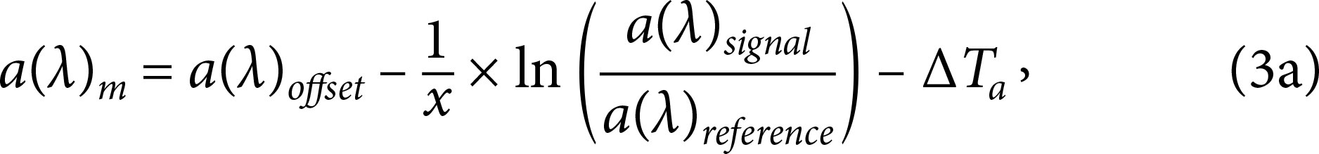
where a(λ)offset is the flow cell/wavelength specific pure water offset obtained from the .dev file, a(λ)signal and a(λ)reference are the flow cell/wavelength specific raw signal and reference counts from the ac-s, x is the path length of the flow cells in meters (defined in the .dev file), ∆T is the flow cell/wavelength/temperature specific temperature bin offset found in the .dev, which is linearly interpolated using the internal temperature of the instrument, and a(λ)m represents the measured signal in m–1, which may be further corrected for the spectrum discontinuity inherent in ac-s data at a user’s discretion.
Spectrum Discontinuity Correction
The ac-s Protocol describes a “spectral stair-step” that occurs randomly and is largely influenced by the particles in the seawater being measured (Sea-Bird Scientific, 2011, Rev. Q, Section 5.8.2). A review of an ac-s absorption or attenuation spectrum at any point in time and in any medium most frequently reveals a sharp discontinuity typically between 550 nm and 580 nm in signal counts and reference counts, and consequently in measured values (Figure 1). This discontinuity jump can typically be found programmatically at the location of the minimum difference between the absorption and attenuation wavelength bins (Wingard et al., 2023). This jump is stated to occur from a timing difference associated with the split filters on the rotating filter wheel, meaning that the flow in the sampling volume slightly advances during filter transition. This would then mean that each half of a spectrum represents different water “masses,” where particulate, dissolved, or bubble quantities may differ in a short period of time (tens of milliseconds) (Sea-Bird Scientific, 2011). It is also hypothesized that random mechanical sources may also contribute, such as wobbling within the filter wheel as it rotates, but to a degree less apparent than a change in water properties.
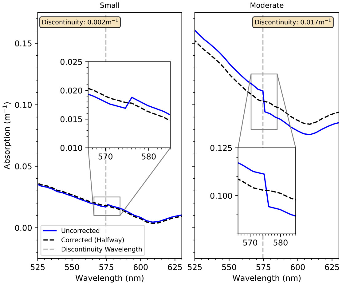
FIGURE 1. Discontinuity example for an absorption spectrum. The left subplot shows a small, typical spectrum discontinuity offset. The right subplot displays an example of a moderate discontinuity offset. In this figure, the discontinuity is corrected by shifting both halves to meet in the middle (the “halfway” method). > High res figure
|
Application of a discontinuity correction on measured values is practical considering that the computation uses both signal and reference counts. The difference in correcting spectra for this discontinuity on raw counts compared to the measured value spectra is likely negligible. Correction of this stair-step is not a well-documented process for an individual spectrum, and the general recommendation from Sea-Bird is to average spectra to remove the discontinuity. This discontinuity is effectively removed during user-initiated data binning/averaging steps (Sea-Bird Scientific, 2011), but users interested in using data for fine-scale, high-resolution analysis may want to smooth or apply a correction to each individual spectrum. Some have implemented a cubic spline to calculate a scalar offset for each individual spectrum (Bausell, 2019), which is then applied to values at wavelengths greater than the discontinuity wavelength. Other options for creating a contiguous spectrum include applying the offset to the first half of the spectrum, or by shifting both halves to meet halfway (which is the default functionality in acspype).
Discontinuity jumps appear to vary in magnitude and direction, even within the same ac-s deployment. A review of datasets we collected aboard NOAA Ship Shimada shows a wide range of absorption discontinuity offsets (0–15 m–1). Looking more closely at these offsets and the associated spectra, it is clear that offset values larger than the maximum of the dynamic range of the sensor (10 m–1) are associated with spectra that are excessively noisy (likely due to bubbles or a quick transition to particle-laden water) and can already be considered poor quality through quality assessment and quality control (QAQC) tests, such as the gross range or absorption-greater-than-attenuation test.
The maximum precision of the ac-s instrument is ±0.003 m–1 (Sea-Bird Scientific, 2023). Spectra with discontinuity offsets within this precision can likely be made contiguous using the halfway correction method without significant fear of downstream effects on data products. Discontinuity offsets greater than ±0.003 m–1 may be questionable and offsets greater than the instrument accuracy (±0.010 m–1) should be treated as highly suspect, as they may indicate a rapid transition in the optical properties of seawater or possibly some sort of stochastic misalignment in components.
Temperature-Salinity Dependence
The conversion and correction of data up to this point are done without the assistance of ancillary data. Correction for the temperature and salinity (TS) of the measured seawater is a necessity (Equation 4a; Sea-Bird Scientific, 2011). At shorter wavelengths (<550 nm), there isn’t a strong dependence on TS. However, at wavelengths longer than 550 nm, absorption dependence on TS exhibits several peaks and troughs (Sullivan et al., 2006) that modulate the relative contribution of seawater when later deriving the particulate and dissolved contributions. The coefficients given in Table 1 of Sullivan et al. (2006) are most commonly used in TS correction and are provided by Sea-Bird Scientific in a TS4.cor text file that accompanies each ac-s and factory software program. acspype provides these values interpolated to 0.1 nm bins for quick lookup. It has also been observed that some ac-s instruments arrive from the factory with wavelength bins less than 400 nm, which are wavelengths not supported in the TS4.cor file. Although they could be considered small and negligibly different from values around 400 nm, we have extrapolated the Sullivan et al. (2006) coefficients down to 395 nm so that such data are not at risk of being lost during this processing stage. Equation 4a provides the TS correction for absorption.

where a(λ)m is derived from Equation 3a, ψt and ψSA (psi_t and psi_s_a) are absorption-specific temperature-salinity dependences found in the TS4.cor file, temperature (T, °C) and salinity (S, PSU) are from a co-located CTD instrument or thermosalinograph, Tref is the tcal (or sometimes Tcal) value found in the corresponding ac-s .dev file, and a(λ)mts is the resulting measured value corrected for the temperature and salinity of the seawater.
Absorption Scattering Correction and Wavelength Interpolation
Sea-Bird Scientific emphasizes three methods for correcting absorption for the effect of scattering within the absorption flow cell of the instrument (Sea-Bird Scientific, 2011). Method 1 is known as the baseline (or flat) method and simply assumes that absorption is zero at a longer wavelength (traditionally 715 nm, based on past work with the WETLabs AC9; Zaneveld et al., 1994; Equation 5.1a). However, the first red wavelength (>700 nm) to approach zero and remain positive may be acceptable over implementing a negative value as the reference. The interactive ac-s processing software InLineAnalysis (Bourdin et al., 2024) provides an option for dynamically identifying an optimal reference wavelength, which acspype mimics. Method 2, known as the fixed method, removes a fixed proportion of the volume scattering function (ε) based on the subtraction of absorption from attenuation (Zaneveld et al., 1994; Pegau et al., 2003; Stockley et al., 2017; Equation 5.2a). The fixed method requires knowledge of the dominant particle type (sediment vs. phytoplankton) in the sampled seawater and is not well suited as an unsupervised correction for ac-s data that may represent different water masses. Method 3, known as the proportional method, effectively combines Methods 1 and 2, with reference wavelength values for both absorption and attenuation defining the proportion of scattering (Zaneveld et al., 1994; Equation 5.3a). All three methods, along with newer correction methods such as the proportional+ method (Röttgers et al., 2013), are provided to give users flexibility in choosing a preferred scattering correction or the option of computing all simultaneously for comparison. Figure 2 offers a visual representation of the effect of scattering correction Methods 1–3 on an absorption spectrum.
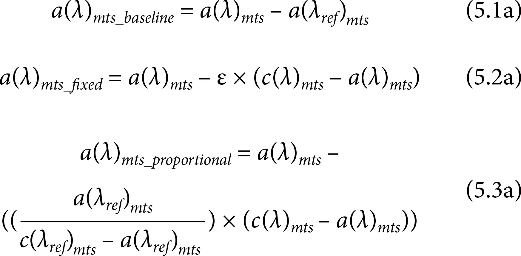
where a(λ)mts and c(λ)mts are derived following Equation 4a, λref indicates the value at the reference wavelength for attenuation or absorption (usually 715 nm), and ε is an empirical coefficient selected by the user (typically between 0.14 and 0.18).
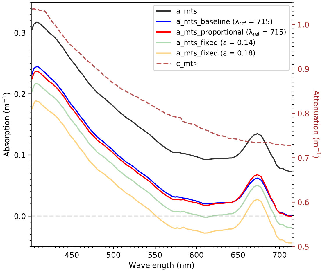
FIGURE 2. Example spectrum showing the effect of temperature-salinity, baseline, fixed, and proportional corrections. > High res figure
|
acspype also provides functions for linearly interpolating a dataset to common wavelength bins, with a default range inferred from the minimum and maximum wavelength values found in a device file with a default step size of 1 nm. Linearly interpolating to common bins is necessary for performing wavelength-indexed scattering correction using xarray and for the merging of datasets from different ac-s instruments after proper correction and user calibration. It is predicted that linearly interpolating between wavelengths is an adequate practice, unless the spectrum is excessively noisy, in which case it should have been previously flagged using QAQC tests (see below).
Quality Assurance and Control (QAQC) and Uncertainty Propagation
acspype offers several quality assessment tests that can be run on ac-s data, with outputs that match the Quality Assurance/Control of Real Time Oceanographic Data (QARTOD) to flag meanings (IOOS, 2020). Some of the tests provided through acspype are diagnostic and only applicable to the ac-s, such as the internal temperature test, which flags data outside the range of the internal thermistor. Tests like the gross range test provide a flag value for each sample at each wavelength. For users who prefer a single flag for each spectrum, blanket tests are provided; however, the appropriate flag conditions should be explored before running such tests unsupervised. The settings used for quality assessment and the removal of flagged data are left up to the user, although we do provide recommended default values and code examples for removing flagged data. For example, a user may opt to set a smaller range for the user_min and user_max values for the gross range test to identify values of high interest, rather than defining data as suspect.
acspype contains functionality for estimating uncertainty and its propagation through each processing step. Internally, the uncertainties Python package (Lebigot et al., 2025) is used for estimating uncertainty following linear error propagation theory and takes into account the manufacturer-noted precision/accuracy values (Csavina et al., 2017) associated with the ac-s and the standard deviations for pure water measurements provided by Sullivan et al. (2006). For propagation into TS correction, users will need to supply the known accuracy of the temperature and salinity measurements, although it is anticipated that uncertainty in those ancillary measurements does not contribute an alarming amount to the overall uncertainty of an absorption or attenuation measurement (Figure 3). The primary contributor to uncertainty in ac-s measurements is the base uncertainty associated with the instrument’s accuracy and precision. As a first order estimate, an uncertainty of ±0.015 m–1 at the TS-correction stage may be reasonable if users do not want to track and calculate uncertainty at each processing stage for each spectrum. Of course, this does not account for uncertainty associated with the long-term stability of the ac-s.
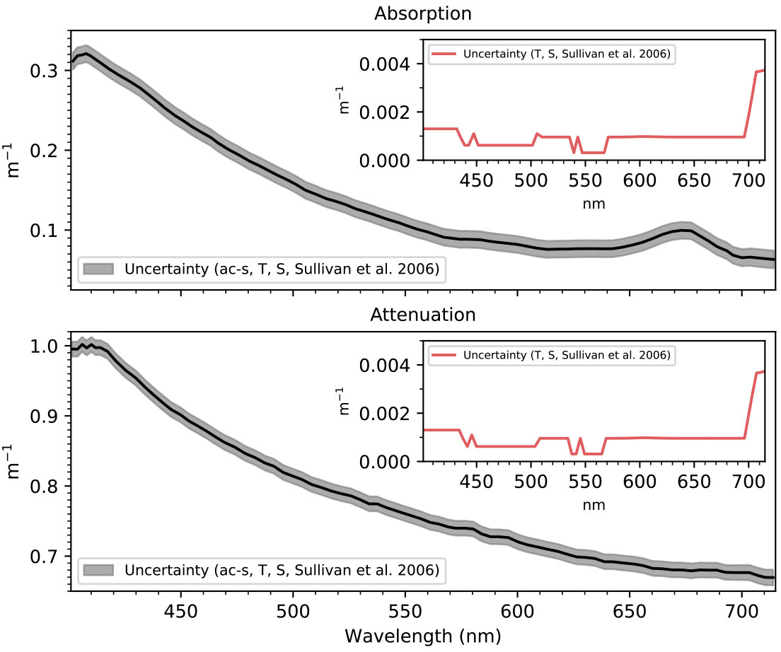
FIGURE 3. Example of uncertainty across an absorption and attenuation spectrum. The gray infill is uncertainty that propagates up through the temperature-salinity correction and considers the base uncertainty of the ac-s, including an estimated accuracy for the internal thermistor of 0.1°C (Sea-Bird Scientific, pers. comm., 2025), an uncertainty of 0.2°C and 0.2 PSU, and the uncertainty in the measurements from Sullivan et al. (2006). The inset axes represent the approximate contribution to uncertainty if only considering temperature, salinity, and the Sullivan et al. (2006) uncertainties for a temperature of 13.42°C and a salinity of 31.0 PSU. > High res figure
|
Workflows
Required and optional (encouraged) steps for processing and assessing ac-s data from raw values to geophysical quantities to derived biogeochemical data products have been aggregated and compiled into a set of living tables in the acspype repository. A few methods for computing derived and empirical data products, such as POC and chlorophyll a from absorption line height are also included in the software. Example workflows are also provided in Figure 4 and described further in the package repository. Code documentation for functions and modules that perform these steps can also be found on GitHub. Processing up through the temperature-salinity corrected coefficients, if ancillary data are available, can be done reliably within the time between full serial packet retrieval on most computers (~250 ms); this offers a reasonable data product level to provide to end users in real-time for visualization (Figure 4).
For those looking to redistribute ac-s data to the public as archived datasets, it is recommended that data be corrected at least through the proportional scattering correction with a reference wavelength of 715 nm in order to be consistent with past literature and accompanied by relevant quality assessment test results and uncertainty estimates.
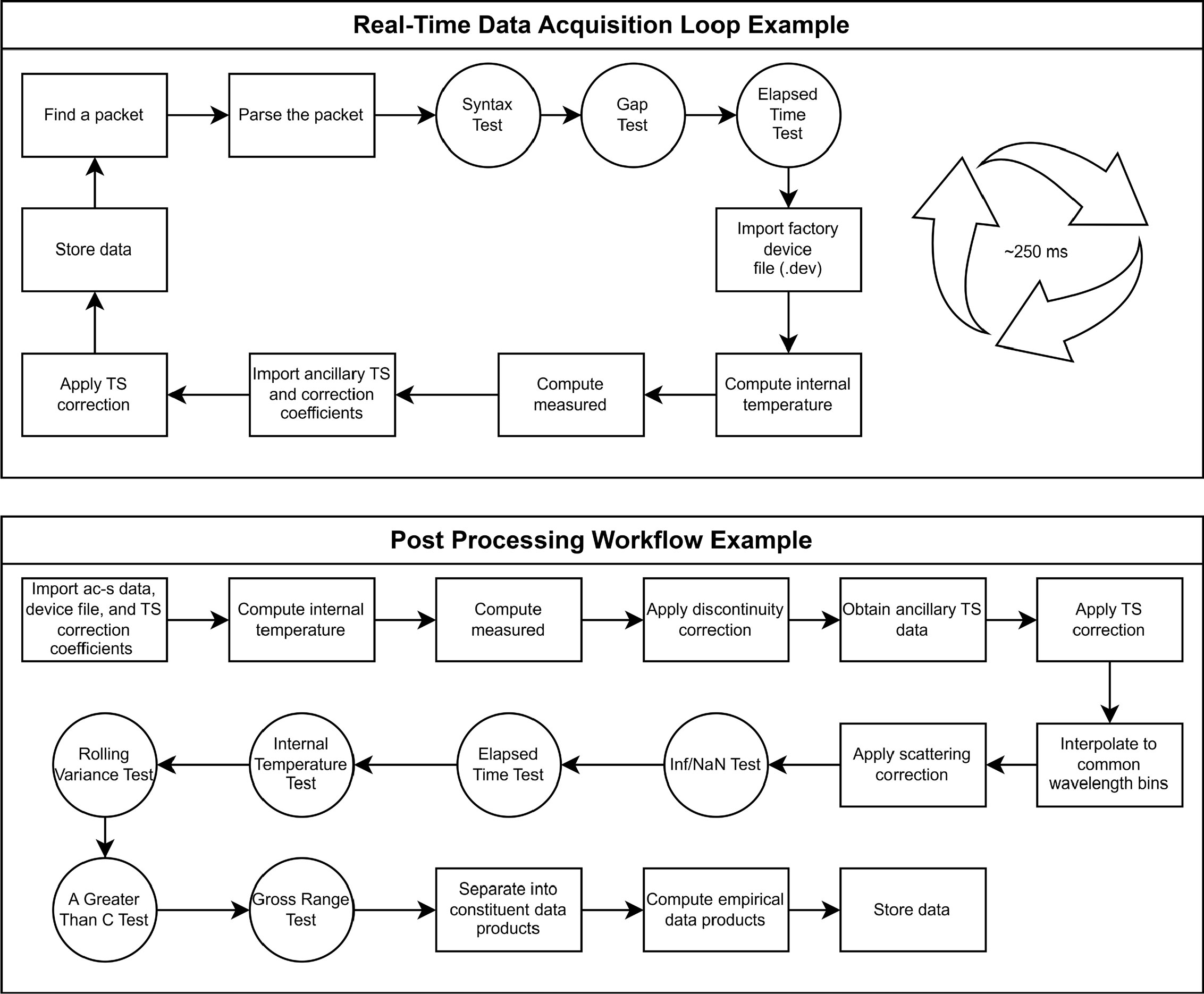
FIGURE 4. Example workflows for real-time ac-s data acquisition and post-processing. A living document containing descriptions of processing steps can be found in the project repository. > High res figure
|
Conclusion and Future Development
acspype provides Python users with the ability to acquire and process ac-s data in intuitively written programs and formats. Through this work, steps described in manufacturer documents and scientific literature were synthesized and codified for general application of ac-s data in real time and for archived datasets. QAQC tests are provided to aid users in rapidly identifying poor and suspect quality data that are largely related to instrument malfunction. Integration of acspype into processing and acquisition scripts will make base data and derived data products easier to navigate for end users and will speed up the task of making these data accessible.
acspype currently lacks functionality for performing time-lag correction with ancillary datasets in flowthrough, as well as spectrum alignment for ac-s sensors that have flow cells plumbed in series. These additions are needed for applications that require fine-scale particle analysis in very small time and depth bins or on a spectrum-by-spectrum basis. acspype would also benefit from additional functions that assist with uncertainty estimation, such as uncertainty associated with fluctuation of the measurement over time (Waldmann et al., 2022). Users are encouraged to submit requests, concerns, issues, and their own contributions on GitHub.
Code and Examples
acspype is open-source software and available on the Python Package Index for Python 3 (≥3.10). All code and examples can be found on the main branch of the GitHub repository. Code and module documentation is also hosted on GitHub. Additional information, such as QAQC test descriptions, recommended naming conventions, processing steps, and reference material are also provided in the repository and will be updated periodically.
Acknowledgments
Thank you to Clare Reimers for providing support and feedback on the initial stages of the manuscript. NSF provided salary support for ITB during the preparation of this work under award number OCE-1748726. MTK was supported by NASA Award Number 80NSSC20M0008 and NOAA Award Number NA24NOSX012C0022-T1-01. Thank you to Russell Desiderio, Andrew Barnard, and our anonymous reviewers for providing feedback on the later stages of the manuscript. The efforts of Nils Haëntjens and Chris Wingard to create open-source software are appreciated and influenced the development of acspype. Many thanks to Kelly George for collecting ac-s data aboard NOAA Ship Shimada, which was used in the development of this package and the figures in this manuscript.