INTRODUCTION
Oceanography relies on a wide range of observational platforms, sampling strategies, and experimental and modeling approaches to drive discovery and deepen our understanding of the ocean’s role in the Earth system (Lee et al., 2017; McMahon et al., 2021). Over the past few decades, there has been a significant increase in both the volume and variety of oceanographic data (Tanhua et al., 2019; Brett et al., 2020). Advancements in computational power over the last decade have further enhanced the efficacy of models, fueling a surge in modeling studies (Stewart and Thompson, 2015; Morrison et al., 2020; Huneke et al., 2022). As a result, computational methods and resources are becoming essential tools in oceanography (Reichstein et al., 2019; Robinson et al., 2020), with numerous examples of advanced computational usage across the field (Hemming et al., 2020; Kiss et al., 2020; Chapman et al., 2022; Roughan et al., 2022).
Despite these advancements, ocean science courses have traditionally focused on domain-specific knowledge, often lacking comprehensive training in computational skills (Campbell et al., 2024). Though introductory-level data science training is increasingly being incorporated into oceanography curricula, students and researchers are left with significant gaps in advanced computational skills (Greengrove et al., 2020; McGovern and Allen, 2021). The education and equipment required to develop these computational skills can be expensive and time consuming (Barber et al., 2023), with marginalized students often forced to forgo training opportunities and internships (Kreuser et al., 2023). Scientific programming skills, particularly the ability to collaborate effectively on computational projects, are highly valuable in both academic and non-lab-work environments (McNutt, 2014).
OceanHackWeek was established in 2018 with three core goals: (1) to provide a pathway for ocean scientists to acquire the computational and data science skills necessary for advancing modern data-intensive oceanographic research; (2) to foster an open and sharing culture among ocean science researchers, spanning a wide range of technical expertise, career stages, educational backgrounds, and personal experiences; and (3) to promote open science, reproducible research practices, and adherence to FAIR (findable, accessible, interoperable, reusable) data principles. Open, reproducible science encourages greater inclusivity, enabling broader participation from researchers worldwide and creating opportunities to engage in groundbreaking science, regardless of institutional affiliations or financial resources (Martin et al., 2025). In this paper, we focus our main discussion on the OceanHackWeek event, with details on the organization of OceanHackWeek provided in the online Supplementary Materials.
THE OCEANHACKWEEK WORKSHOP
The hackweek model (Duncombe, 2018; Huppenkothen et al., 2018; Rokem and Benson, 2024) was designed to fill a gap between traditional summer schools, which are typically instructor-led lessons, and hackathons, collaborative events focused on a specific problem. Hackweeks combine instructor-led tutorials and collaborative project work that enables peer learning (Figure 1).
OceanHackWeek originated as an adaptation of this hackweek model and is typically run as a five-day workshop that is a balance between tutorials and project work. The design and scope of the OceanHackWeek event has evolved since its inception, becoming broader and more inclusive over time with the introduction of a virtual option and multiple in-person events in different locations run concurrently—see Supplementary Table S1 and details of OceanHackWeek en Español in Martin et al. (2025). The OceanHackWeek approach emphasizes the value of both scientific research and software contributions, recognizing that science and software development are interconnected forces that drive progress. Diversity is essential in this process, that is, bringing together individuals with varied backgrounds and insights to enrich the research, foster innovation, and create stronger solutions. To ensure broader participation and inclusivity, OceanHackWeek is run at no, or very minimal cost, to the participants. Thanks to the generous support of our sponsors (see list provided in the Acknowledgments section), and the time volunteered by many of the organizers, instructors, and mentors, we have no registration fees, provide accommodation free-of-charge, and subsidize travel and meal costs.
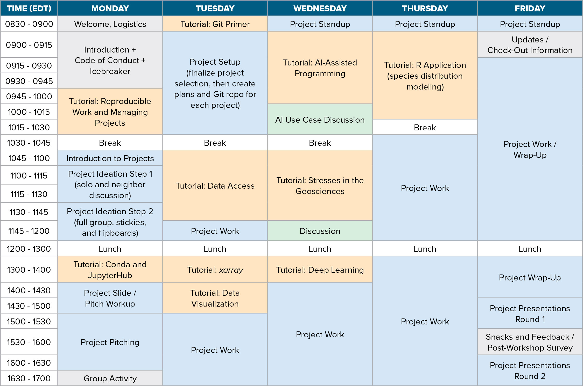
FIGURE 1. Example schedule from the 2024 OceanHackWeek workshop. General activities are in gray, tutorials are in orange, discussions are in green, and project related activities are in blue. > High res figure
|
SOFTWARE AND INFRASTRUCTURE
OceanHackWeek uses both the Python and R programming languages. Initially, the focus was on Python due to its growing prominence in oceanographic research and the broader geosciences (Irving, 2019; Esmaili, 2021), but R was later included, recognizing its importance in ecological and biological research (Lai et al., 2019). We embraced both Python and R because (1) the core computing and data analysis ideas are independent of and transferable between programming languages, (2) many software tools are language-specific and flexibility in switching between languages is advantageous, and (3) working alongside others with expertise in a different language can be inspiring and facilitates collaboration across ocean science sub-domains.
OceanHackWeek has relied on customized JupyterHub deployments hosted on commercial cloud services since its inception, providing a shared platform accessible to all participants through a web browser, in the form of JupyterLab and RStudio interfaces. The platform is provisioned with the software libraries and resources used in the tutorials and light project work and thus provides a consistent environment to all participants.
OceanHackWeek uses GitHub for access to the JupyterHub, sharing of tutorial materials, and collaborative project work. In addition, we use Slack as a communication platform for all event types (in-person, virtual, and hybrid). Each project has a dedicated Slack channel and a GitHub repository, and there are Slack channels for sharing logistics and coding help. A video conferencing platform is necessary for virtual and hybrid events, but we disable the chat feature of these platforms and direct all communication through Slack, in a tutorial Q&A channel.
CURRICULUM OVERVIEW
Figure 1 shows a typical schedule for a five-day OceanHackWeek workshop, beginning with tutorials and project team formation; project time increases as the week progresses. In the early years, our tutorials focused on accessing data from ocean observing networks (e.g., the Ocean Observatories Initiative and the US Integrated Ocean Observing System) or specific software libraries for data manipulation and visualization (such as Python’s xarray). Since 2023, we have included tutorials that demonstrate data analysis challenges associated with research questions and provide participants with a broader overview on how to approach a computational research project. A list of the past tutorials is provided in Table S2, with the majority of these available on GitHub and in recordings on our YouTube channel.
In addition to programming tutorials, we engage participants in sessions on broad, culturally oriented topics including code of conduct in collaborative research, reproducible and replicable research, and open science challenges and ethics, and we host an open discussion session on mental health in climate science. These sessions are important for cultivating an inclusive, collaborative, and open culture.
Projects
Group-based “hack” projects are a crucial component of OceanHackWeek, with learning and collaboration as the goal, rather than complete project solutions. Participants are encouraged to propose (“pitch”) a project and form a project team with other participants. Project goals and individual contributions are negotiated and adjusted throughout the week as challenges arise and time progresses. The week concludes with presentations from each project group, where participants are asked to explain what was accomplished and what lessons were learned, regardless of the original objectives.
Due to the organic nature of project formation, the project groups tend to be diverse in terms of skill levels and domain knowledge. We encourage this, as we have found it results in peer-to-peer learning, with tasks distributed within the team to the appropriate participants. Those with higher coding skill levels often practice their teaching skills by helping others in their group; likewise, participants with a deeper background in the project’s science goals or relevant data sources often provide critical guidance to the group. The group-based setting of the hack projects aims to foster an open and collaborative scientific process, with participants encouraged to continue using these approaches in their work beyond OceanHackWeek. Box 1 shows examples of two OceanHackWeek projects that demonstrate the breadth of the projects. All projects are accessible from the OceanHackWeek website.
BOX 1. EXAMPLE PROJECTS
colocate
The colocate module started as an OceanHackWeek project in 2019 and is now a module managed by the US Integrated Ocean Observing System. The project was created to leverage the efforts of many groups by serving valuable data via common ERDDAP interfaces and a community-maintained index of such servers and enabling a single set of search criteria to be applied across servers. This module has a user interface that is used to search ERDDAP servers in order to locate all oceanographic data within a given region over a set time period (Figure B1-1).
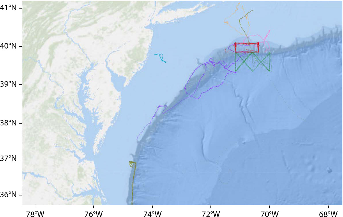
FIGURE B1-1. Results from a colocate search. Different colored lines show where available data have been found. Figure created from code available in the colocate module. > High res figure
Turtle Detection Using Deep Learning
The 2021 Turtle Detection Using Deep Learning project used an established neural network segmentation model to identify turtles in videos taken by drones. This project demonstrates the power of a diverse team, with someone providing the dataset and scientific knowledge behind it, some team members supplying expertise in data wrangling, and others offering experience working with neural networks. Together, in a short period of time, they successfully built a model that identified turtles (Figure B1-2).
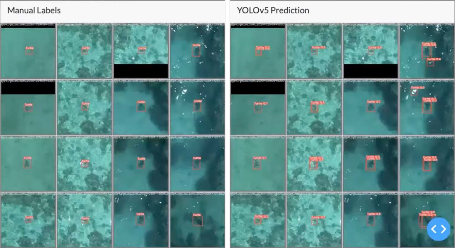
FIGURE B1-2. A screenshot from the video of the turtle detection project presentation identifies turtles detected in the drone imagery. Go to the flipbook version of this article to view the full video. > High res figure
|
APPLICATIONS AND PARTICIPANT SELECTION
We have strived to build a diverse cohort with outreach to applicants from underrepresented groups through institutional, national, and international mailing lists; minority-led societies; and social media. Applications are open to all, but participants are expected to have some experience with Python and/or R. Participants are typically graduate students, but we welcome (and have had) participants from all academic stages, as well as from outside of academia. Over the years we have honed our selection process, settling on a holistic approach to reduce bias and the impact of disparities among applicants that arise from different backgrounds and opportunities (Huppenkothen et al., 2020; Young et al., 2022). Holistic reviews consider a broad range of criteria but minimize dependence on quantitative metrics (such as grade point averages for graduate school admissions) and put a greater emphasis on skills, experiences, and personal attributes (Megginson, 2009; Wilson et al., 2019). In our participant selection, we focus on three categories: motivation (why does an applicant want to participate), impact (what impact OceanHackWeek would have on an applicant’s research interests and beyond), and ability to work in a team. In 2024, we followed the approach of Rotjan et al. (2023), with participants classified as either eligible or ineligible to attend OceanHackWeek, and final participants selected randomly from the eligible pool. In prior years, participants were ranked, with places offered to the highest scoring applicants. We have found the holistic approach to reviewing applicants helps reduce our biases, and coupled with a purposeful outreach, helps OceanHackWeek achieve a diverse cohort.
EVALUATION OF THE PROGRAM AND LESSONS LEARNED
OceanHackWeek conducts a post-workshop survey to assess the success of the workshop and identify areas for improvement. The individual survey responses are confidential, so we present the collective lessons we have learned from seven years of surveys as well as conversations with participants, instructors, mentors, and organizing committee members. The participant testimonials and alumni stories provided in the Supplementary Materials demonstrate the value of the program to these participants, particularly regarding OceanHackWeek’s community-building, positive atmosphere, and the group projects.
Participation and Engagement Across Event Formats
A virtual option for OceanHackWeek enabled the participation of a more diverse and global community. Table S1 shows participant demographics for each workshop, with larger percentages of gender and ethnic/racial minorities, as well as international participants, in the years conducted as fully virtual or hybrid events. Participants appreciated the virtual option, but despite the positive feedback we received regarding the virtual/hybrid model, in the last two years there was less interest in participating virtually, suggesting that participants currently prefer in-person interactions and workshops.
Further, planning and running a hybrid workshop that aims to provide equitable experiences to all the participants, irrespective of their mode of participation, is challenging. To host a successful hybrid workshop requires a lot of additional infrastructure and coordination (Rokem and Benson, 2024). For OceanHackWeek, this includes our standard infrastructure plus a video conferencing platform, consistency in facilitating project work, and any in-person logistics. Given the wide range of tasks, we have found that a large team of organizers is necessary, with some focused on the in-person component and others dedicated to the virtual component. In the case of the “distributed” model with multiple in-person locations, we suggest a separate organizing group for each of the satellites.
Project work in a hybrid setting can be extremely successful but requires significant facilitation—more than a solely in-person or virtual event requires. For most of the projects, in-person and virtual participants interacted with each other and collaborated asynchronously around the clock and around the globe. Participants enjoyed these interactions and working across those traditional boundaries. This success was based on project-facilitator skills and the project-specific communication avenues (dedicated Slack channels) and GitHub repositories available on our shared cloud-based computational platform. The project facilitators helped ensure communication was flowing among all team members by actively checking in with virtual participants to encourage their continuing involvement. We found that if the project team was mostly composed of in-person participants in a single location, it was often harder for the external participants to engage (even with the facilitation).
Fostering an Open, Sharing Culture
Scene setting is important for cultivating a welcoming, inclusive environment. Each year, a collaborative Code of Conduct is developed as one of the workshop’s opening activities, and the website is updated with the new Code of Conduct. In addition, we give a presentation that explains our project philosophy and offers tips for smooth teamwork. We have found these activities help participants feel welcome, encourage participants to be inclusive, and build a supportive environment where participants feel comfortable contributing (see participant testimonials in the Supplementary Materials).
Software
OceanHackWeek projects tend to use one main programming language, although some participants take this as an opportunity to work in their less-dominant language, or in a different sub-domain, to expand their knowledge and skillsets. We have conducted tutorials in both languages, experimenting with duplication of tutorial topics (e.g., “Data access in Python” and “Data access in R”), separate tutorials that focus on a Python- or R-specific tool (e.g., xarray or oce, respectively), and more general tutorials that address a problem and how to approach solving it. As it can be challenging to keep the attention of participants during the tutorials in their non-dominant language, we have found more engagement with the “addressing-a-problem” approach, which tends to be agnostic regarding the language and more about the process.
Using a shared computational environment brings many advantages for this type of workshop (Rokem and Benson, 2024; Sauthoff et al., 2024): we do not need to factor time into our schedule to ensure all the participants have the correct environments installed, allowing us to focus on our learning goals; it helps project teams have consistent environments; and it gives participants the opportunity to (potentially) try out a new coding language without having to install it on their local machines (Martin et al., 2025).
RECOMMENDATIONS
Based on our experience, we offer five recommendations for running an OceanHackWeek style event.
- Conduct a five-day, immersive workshop. Five days allows time for tutorials but still gives participants ample time for project brainstorming, group formation, and project work.
- To promote inclusive, productive project teams, set the scene at the start of the session and check in frequently with participants. For example, discuss tips for effective teamwork and create a code of conduct.
- If the desire is to teach or encourage multiple programming languages, think carefully about the tutorial approach. Language agnostic tutorials are good if everyone is listening to the same tutorial, but if the setting allows, splitting into groups for more language/tool specific tutorials could be beneficial.
- Choose computing infrastructure that works for the program/lesson goals. We recommend a shared computing platform (e.g., a JupyterHub) to minimize time troubleshooting participants’ individual systems. However, depending on the goals (e.g., if one goal is enabling participants to work locally beyond the event), walking through installations and environment setups may be appropriate.
- If the workshop will be hybrid, have materials and clear guidelines to help with facilitation of the event across the different modes of participation. It is important to have a project facilitator for every project, and some organizing committee members focused on either the in-person component or the virtual component rather than having everyone trying to organize both. A virtual-only workshop can provide the benefit of expanded accessibility while reducing the burden of coordination between in-person and virtual modes of participation.
While the discussion in this paper focuses on a five-day workshop format, aspects of OceanHackWeek can be translated to a classroom environment. Indeed, past organizers and participants have already successfully adapted the model to more specific contexts (Martin et al., 2025). Data science and oceanography skills could still be taught with our tutorial and project-work approach but spread out over a different time frame; the group projects could be done in the classroom, or a hackweek could be held within a research team, a department, or an institution.
With more than 450 participants over seven years, OceanHackWeek has catalyzed intellectual and technical exchanges among ocean scientists from diverse backgrounds. The balance of tutorials and participant-driven project work provides attendees with new technical skills and collaboration opportunities that extend beyond the event, accelerating discovery and innovation in the ocean sciences.
Author Contributions
OceanHackWeek is a collaborative project, with each member of the team contributing in many different ways. All authors are/were members of the 2023 and/or 2024 OceanHackWeek Steering Committee, and all have been involved in organizing the annual event for one or more years. For this article specifically, we list roles following the CRediT system: Conceptualization, CM, WL. Writing – original draft and project administration, CM. Writing – review and editing, CM, WL, FF, JG, AK, EM, TM, NM, NR, VS.
Acknowledgments
Over the past seven years, many people have played roles in OceanHackWeek, from shaping the direction of the program to organizing one (or more) of the annual events. There are too many to call out individually, but we are extremely grateful for the contributions of all. We also sincerely appreciate the sponsorship and funding that has supported the event over the past seven years, enabling participants to attend at minimal cost: Integrated Ocean Observing System (IOOS), NSF Division of Ocean Sciences, NASA, Schmidt Ocean Institute, University of Washington eScience Institute, University of Washington Applied Physics Laboratory, Ocean Carbon and Biogeochemistry Program, NOAA Global Ocean Monitoring and Observing, Integrated Marine Observing System (IMOS), Commonwealth Scientific and Industrial Research Organisation (CSIRO), ACCESS-NRI.