Introduction
Rain generates lenses of buoyant fresher water in the upper few meters of the ocean surface that persist for at most a few tens of hours before mixing and advection destratify the surface layer (Brainerd and Gregg, 1997; Wijesekera et al., 1999). Fresh lenses modulate the air-sea fluxes of heat, mass, and momentum, which in turn affects surface heating and currents (Soloviev and Lukas, 2006), air-sea gas exchange (Zappa et al., 2009), and turbulent kinetic energy (TKE) dissipation (Smyth et al., 1996; Soloviev and Schluessel, 2002). Turbulence is critical in destratifying the surface layer, and although wind-related mechanisms (shear stress, wave breaking) dominate the production of TKE at the ocean surface at intermediate and higher wind speeds, experiments conducted in wind-wave tunnels indicate that the impact of raindrops can be a significant source of turbulence at low wind speeds (Harrison et al., 2012; Harrison and Veron, 2017). However, there are few measurements of rain-generated turbulence available for the open ocean, so it is unclear whether rain has a measurable effect on mixing at the ocean surface. Data collected during the month-long field campaign in 2016 for the second Salinity Processes in the Upper Ocean Regional Study (SPURS-2) in the eastern equatorial Pacific Ocean (SPURS-2 Planning Group, 2015) allow investigation of this question.
One of the main science questions to be answered by SPURS-2 is which physical processes are most important in generating vertical and horizontal variability in upper-ocean salinity in regions with large freshwater inputs from rain. Understanding the mechanisms controlling the formation and evolution of the surface fresh layer that are associated with rain is an important part of SPURS-2. This includes measuring the turbulence generated at the surface of the ocean by rain. However, as demonstrated by Zappa et al. (2009), this turbulence is likely confined to a ~10 cm layer below the ocean surface that has a steep vertical gradient in TKE dissipation. State-of-the-art instruments for measuring turbulence cannot quantify turbulence above a few centimeters in depth (Thomson, 2012) and thus are unsuitable for observing turbulence generated by rain at the surface of the ocean. However, Zappa et al. (2009) demonstrated that the active controlled flux technique (ACFT; Asher et al., 2004) is effective in estimating rain-generated surface turbulence.
“The active controlled flux technique measurements made in the presence of rain demonstrate that rain has a measurable effect on turbulence in the upper centimeter of the ocean, but that this effect diminishes as wind speed increases.”
ACFT uses infrared (IR) imagery to track the decrease in temperature of a small patch of the sea surface that has been heated a few degrees above the bulk temperature using a short pulse of IR radiation from a laser (Haußecker et al., 1995; Asher et al., 2004). This heated patch has an initial depth on order of a hundred micrometers and cools as heat is transported by turbulence into the cooler bulk water below. One conceptual model for this heat transport is surface renewal, which postulates that turbulence causes the replacement of small elements of the surface with bulk water (Danckwerts, 1950). This implies that the decay rate of the temperature in the heated patch is proportional to the surface renewal rate (Haußecker et al., 1995; Asher et al., 2004; Atmane et al., 2004). Because of the relationship between the surface renewal rate and the turbulence dissipation rate (Lamont and Scott, 1970; Zappa et al., 2003, 2009), ACFT can be used to estimate relative levels of TKE dissipation at the sea surface.
Ocean surface turbulence was measured using ACFT during the 2016 SPURS-2 field experiment. This paper discusses the implementation of ACFT on board R/V Roger Revelle, analysis of the IR imagery, and the results from the measurements. These data will be used to understand the effect that rainfall has on near-surface turbulence and to investigate the relationship between turbulence, rain rate, and wind speed over spatial scales of a few kilometers and timescales on order of a few minutes.
Methods
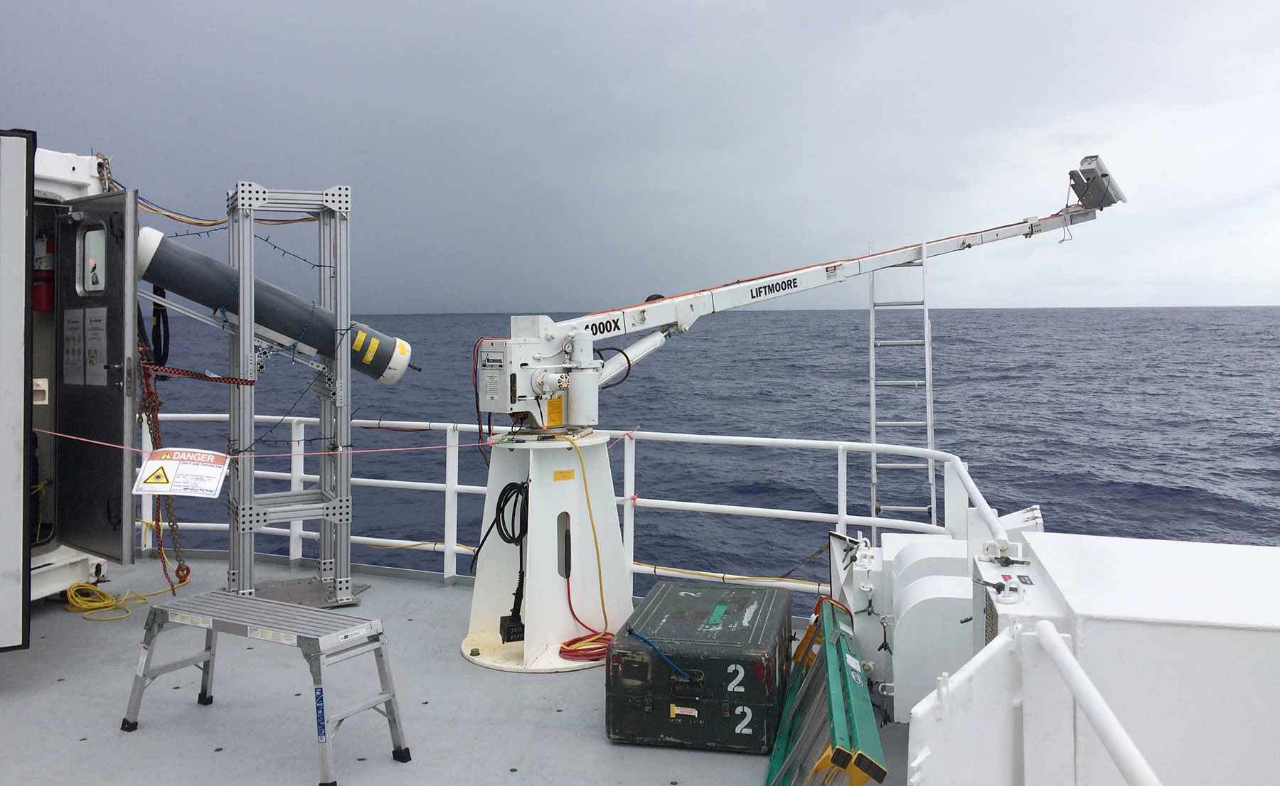
ACFT was implemented during SPURS-2 using a technique similar to that described by Asher et al. (2004). In brief, a 0.1 s pulse from a 125 W carbon dioxide (CO2) laser heated a patch of water on the ocean surface approximately 0.1 m in diameter and 100 μm deep a few degrees Kelvin above the bulk water temperature (where the depth of the patch is defined by the diffusive length scale of heat over the laser pulse width). The heated patch was tracked using an infrared imager (FL 640 QLW, Aeg Infrarot-Module GmbH, Heilbronn, Germany) that was mounted in a weatherproof housing on the end of an electrically operated extendable 6 m boom (4000X-20, Liftmoore, Houston, Texas). The boom was extended outboard of the ship at a height of 10 m above the mean water surface, giving an incidence angle of the imager of approximately 35°. That geometry resulted in a 5 m × 4 m trapezoidal imaged area of the ocean surface. Each image was 640 pixels × 512 pixels, so that the size of the patch in the IR images started out approximately 12 pixels in diameter.
The imager recorded 15 frames per second and the laser provided one pulse every 2 s. The laser pulse and the timing of the images and the laser were synchronized by triggering the laser and imager using the output of a matched pair of digital pulse generators (USBPulse100, Elan Digital Systems Ltd., Fareham, UK). Temporal jitter of the pulse generators was negligible in terms of the temporal width of the laser pulse, the repetition rate of the laser, or the frame rate of the imager, so it was assumed the laser pulse and the imager were synchronized in time.
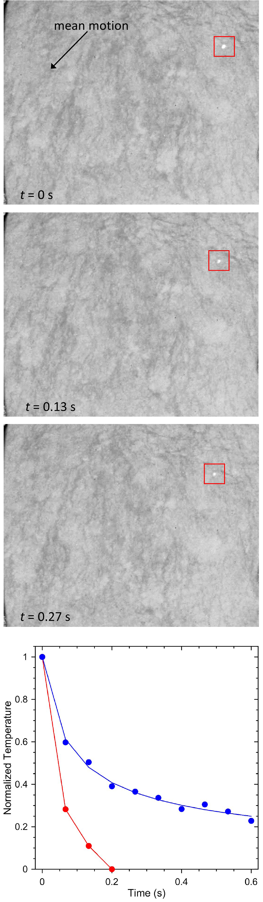
ACFT measurements were made when the ship was towing the surface salinity profiler (SSP) at 2 m s–1, measuring water temperature and salinity at depths of 0.02 m, 0.12 m, 0.23 m, 0.54 m, and 1.1 m, and temperature and conductivity microstructure at a depth of 0.35 m (see Drushka et al., 2019, in this issue, for a complete discussion of the SSP). At 2 m s–1 the laser-heated patch of water remained in the imager field-of-view for approximately 2 s (or 30 images). However, the average decay time for a patch was typically 0.5 s, so ship motion did not limit tracking. The top panels of Figure 1 show a series of three IR images that illustrate how the heated patch cooled and moved downward and to the left through the image sequence with the mean motion of the ship. The bottom panel of Figure 1 shows two representative time series of the patch temperature taken from the data shown in Figure 2 (see below).
|
|
Figure 1. Typical infrared images of the ocean surface showing the location and motion of a patch of water heated by a CO2 laser. The patch is shown inside the red boxes in the upper right quadrants of the time-labeled images. When rectified, each image is a trapezoidal area of the ocean surface that is 5 m wide at the top, 4.75 m along each side, and 4 m wide at the bottom. The typical temperature increase of a patch was approximately 4°C, and the total temperature difference between the coolest (darkest) and warmest (brightest) parts of each image was approximately 5°C. The bottom panel shows two time series of the normalized patch temperature as calculated using the tracking algorithm described in the text. The conditions, the same for each patch, are shown in Figure 2 (approx. 23:25 UTC, YD 254), which indicates that there was significant variability in decay times between laser pulses even without large variability in wind speed. > High res figure
|
To track the heated patches over time, IR images were segmented based on grayscale intensity, with the location of the initial patch in the series of a single laser pulse identified by finding a 3 × 3 set of pixels with an average intensity that was 2.5 standard deviations above the mean intensity of the image. Once the initial location of the patch was identified, the location of each successive patch was tracked in a 50 × 50 box around the previous patch until the mean of the 3 × 3 grid around the brightest pixel in the box was less than one standard deviation above the image mean. This method was found to detect and track over 90% of the patches with approximately 95% of the detected patches tracked until they could no longer be observed by visual inspection of the image. The patch temperature was recorded as the mean of the 3 × 3 box containing the brightest pixel in the interrogation region. The location of the 50 × 50 interrogation region around the patch is shown as the red box around the heated patch in each image in Figure 1.
The absolute brightness values of the patch were normalized using the initial brightness for that sequence producing a temperature decay curve. Each decay curve was fit to the function for the decay in patch temperature given by Veron et al. (2011; see their Equation 5) to extract the penetration depth, h (m), and surface renewal time constant, τ (s). This time constant is used to calculate the net heat transfer velocity, kH, as
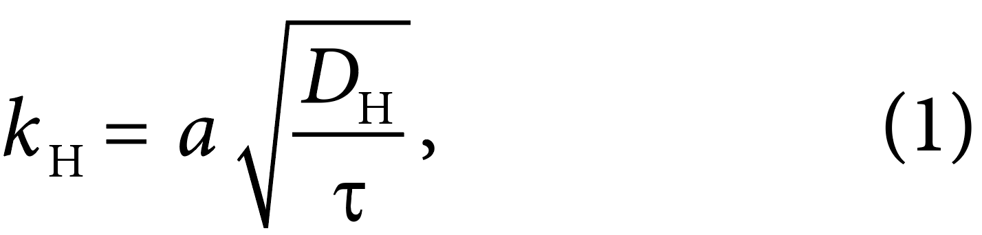
where a is a constant often assumed to be equal to unity and DH is the molecular diffusivity of heat in water (m2 s–1). Zappa et al. (2009) showed experimentally that in the presence of rain, τ was proportional to the turbulence dissipation rate, ε, using the relation
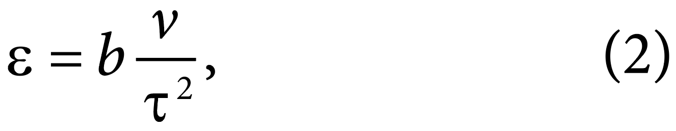
where b is an empirical constant and ν is the kinematic viscosity of water (m2 s–1) (note that this relationship has been proposed many times in the literature, most notably by Lamont and Scott (1970)). By combining Equations 1 and 2, it is evident that ε is proportional to kH4. Because a and b are not known definitively, the quantity τ–1/2 will be used here in place of both kH and ε because it scales linearly with kH.
ACFT was originally developed to estimate the transfer velocity for water-side rate-controlled gases such as CO2. However, both air- and water-side processes affect heat exchange (Soloviev and Schlüssel, 1994; Veron et al., 2011), and there is ongoing debate within the air-sea interaction community about which mechanisms are responsible for the temperature decay at various temporal and spatial scales. Several previous studies have shown that the temperature decay rates measured using ACFT correlate with independent measurements of water-side turbulence (Zappa et al., 2003, 2009), microbreaking and mean-square-slope (Zappa et al., 2004), and wind stress (Asher et al., 2004; Atmane et al., 2004; Veron et al., 2011). This investigation assumes that the heated patch cools mostly through transfer of heat into the water due to turbulence at the water surface. Even if air-side processes contribute to the decay, water-side turbulence is expected to strongly impact the decay rate such that the measured renewal times can be used to investigate the effect of rainfall on the generation of turbulence in the water at the ocean surface.
A minimum of three data points in the temperature decay curve is required to be able to determine h and τ. This condition was met for approximately 80% of the laser pulses; some curves were rejected because although the patch was visible for many frames, the tracking algorithm lost the patch after the first two images, and some curves were rejected because the decay was so fast that the patch was gone after two frames. The raw time series for τ–1/2 with a 2 s data spacing was smoothed by averaging 30 successive values to give a response time of approximately 60 s. Images were collected over the entire 12-hour-long deployment of the SSP in the form of one-hour long sets of images. A total of 96 hours of ACFT data were analyzed here.
Meteorological data for the 2016 SPURS-2 experiment were provided by Clayson et al. (2019, in this issue) as 60 s averaged values and are used without further modification. Because the ACFT measurement times were not synchronized with the meteorological data, values for wind speed, U10 (m s–1), and rain rate, R (mm hr–1), contemporaneous with the ACFT data, were generated by interpolating the 60 s averaged meteorological data onto the ACFT measurement times. The dependence of turbulence on wind speed and rain rate was studied by binning τ–1/2 as a function of U10 or R, respectively.
Results and Discussion
Figure 2 is a 2.9-hour-long time series of τ−1/2, U10, downwelling shortwave radiation, ΦSW (W m–2), and ocean surface water temperature measured by the SSP at depths of 0.02 m, 0.12 m, 0.23 m, 0.54 m, and 1.1 m (T0.02, T0.12, T0.23, T0.54, and T1.1, respectively). The measurements were made under conditions with low winds, clear skies, and no rain. The high downwelling shortwave radiation and low winds led to the formation of a diurnal warm layer (DWL) with a well-mixed surface warm layer between the surface and 0.23 m, and then a vertical gradient in temperature between 0.23 m and 1.1 m. Figure 2b shows ΦSW is correlated with the presence of the DWL. During this period the time series for τ–1/2 shows large sinusoidal oscillations with an approximate period of 20 minutes, corresponding to a distance of approximately 2.4 km. However, U10 is relatively constant over this interval, implying the oscillations in τ–1/2 represent the effect of turbulence that was generated at the ocean surface by a process unrelated to the wind stress. One possible explanation, given the 2.4 km length scale of these oscillations and the fact that they appeared when a DWL was present, is that they are caused by internal waves modulating mixing in the upper few meters of the ocean surface (Walsh et al., 1998; Farrar et al., 2007; Hodges and Fratantoni, 2014). This is supported by the temperature data from the SSP, which show oscillations in temperature in the DWL over the same time period (i.e., 22:19 UTC through 23:17 UTC) as the oscillations in τ–1/2. Note that the features in temperature and τ–1/2 do not align precisely in time or scale because the SSP is measuring the internal wave signature on the DWL. In contrast, the ACFT is measuring the result of mixing in the DWL that is induced by the internal waves. As Farrar et al. (2007) and Hodges and Fratantoni (2014) discuss, there is not a simple correlation between these two effects in terms of temporal and spatial scales. A more detailed discussion of this phenomenon is beyond the scope of this paper.
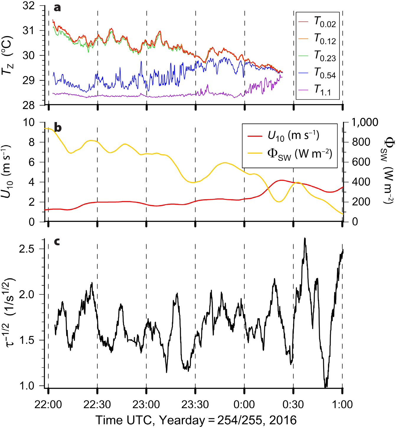
Figure 2. (a) Time series of ocean surface temperature measured by the surface salinity profiler (SSP) at depths of 0.02 m, 0.12 m, 0.23 m, 0.54 m, and 1.1 m (T0.02, T0.12, T0.23, T0.54, and T1.1, respectively). (b) Wind speed, U10, and downwelling shortwave energy flux, ΦSW. (c) Inverse of the square root of the decay time constant measured by the active controlled flux technique, τ–1/2, under conditions of low wind and surface warming. Panel (a) shows the presence of a diurnal warm layer with increasing temperature between 1.0 m and 0.2 m, with a well-mixed warmer layer above 0.2 m. The presence of internal waves is inferred from the periodic increases in T0.54 between 22:19 UTC and 23:17 UTC with corresponding increases in kH during the same period. No rain was measured during this time period so instantaneous rain rate is not shown. The average value for τ–1/2 over this time period was 1.71 1/s1/2, and the mean wind speed was 2.36 m s–1. > High res figure
|
Figure 3 is a time series of τ–1/2, U10, R, and ocean surface salinity measured by the SSP at depths of 0.02 m, 0.12 m, 0.23 m, 0.54 m, and 1.1 m (S0.02, S0.12, S0.23, S0.54, and S1.1, respectively), for a 2.9-hour-long period when there were several rain events with local maxima in R at 06:36 UTC, 06:50 UTC, 07:05 UTC, and 07:28 UTC. The salinity data from the SSP (Figure 3a) shows the presence of a rain-generated fresh lens from 06:28 UTC through 07:40 UTC with a maximum surface freshening at 06:43 UTC.
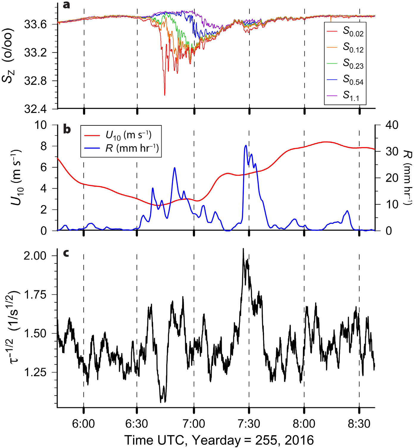
Figure 3. (a) Time series of ocean surface salinity measured by the SSP at depths of 0.02 m, 0.12 m, 0.23 m, 0.54 m, and 1.1 m, (S0.02, S0.12, S0.23, S0.54, and S1.1, respectively). (b) Wind speed, U10, and instantaneous rain rate, R. (c) Inverse of the square root of the decay time constant measured by the active controlled flux technique, τ–1/2, under rainy conditions. The top plot shows the presence of a rain-generated fresh lens with decreasing salinity between 1.0 m and the surface between 06:30 UTC and 08:00 UTC. Local increases in kH are correlated with local peaks in R during this same period. The average value for τ–1/2 over this time period was 1.48 1/s1/2 and the mean wind speed was 5.31 m s–1. > High res figure
|
Qualitative analysis of the τ–1/2 data shown in Figure 3 indicates that when U10 is less than 5 m s–1 and there is a local maximum in R greater than 5 mm hr–1, there is a corresponding increase in τ–1/2 correlated roughly in time with the peak in the rain rate. Maxima in R at 06:36 UTC, 06:50 UTC, and 07:28 UTC have corresponding maxima in τ–1/2 that occur nearly simultaneously. This is consistent with the hypothesis that the impact of raindrops on the ocean surface generates turbulence that increases the decay rate of temperature in the heated patch (causing an increase in τ–1/2). However, after 07:41 UTC, wind speed increases above 5 m s–1 and the two smaller rain events at 07:55 UTC and 08:24 UTC have little effect on τ–1/2.
The average effect of wind and rain on τ–1/2 (and, by inference, turbulence) can be studied by sorting and binning the one-minute averaged τ–1/2, R, and U10 values (a small sample of which are shown as time series in Figures 2 and 3). We determined the effect of wind by sorting the data first by R to separate raining from non-raining cases, using a threshold of R > 0.1 mm hr–1. Then, each set of τ–1/2 and U10 (i.e., for the raining and not-raining cases) was sorted in terms of U10. This produced a sequence of U10 values, each with a corresponding τ–1/2, that could be bin-averaged over 50 sequential wind speeds to produce a mean τ–1/2 and mean U10 as a function of increasing wind speed with and without the effects of rain. Figure 4 shows the result of this binning procedure for the non-raining case to see if the wind speed dependence of τ–1/2 agrees with previous measurements. The solid black line in the figure is the regression line of ACFT measurements of τ–1/2 versus U10 made during the GASEX-01 field campaign, which had non-raining conditions (Asher et al., 2004). The dashed red line shows a linear regression of the SPURS-2 ACFT data for U10 > 5 m s–1 with the solid red lines showing the 95% confidence intervals of the regression.
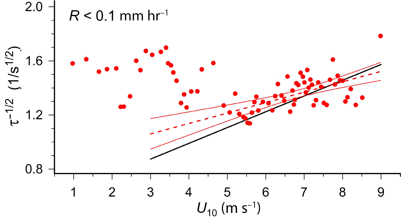
Figure 4. The dependence of the square root of the decay time constant measured by the active controlled flux technique, τ–1/2, on wind speed, U10, in the absence of rain for the 2016 SPURS-2 active controlled flux technique (ACFT) measurements. The data have been restricted to times when the instantaneous rain rate was less than 0.1 mm hr–1. The τ–1/2 values have been bin-averaged as a function of U10 as described in the text. The dashed red line shows the result of a linear regression of the SPURS-2 ACFT results for U10 >5 m s–1. The solid red lines are the confidence intervals (95%) for the linear regression. This regression found that τ–1/2 (1/s1/2) = 0.0772U10 + 0.828 for U10 in meters per second with a coefficient of determination of 0.36. The solid black line is the least-squares linear regression of the ACFT measurements made during the GASEX-01 experiment (Asher et al., 2004) over the same limits as the SPURS-2 ACFT data. The GASEX-01 regression line is τ–1/2 (1/s1/2) = 0.117U10 + 0.524 for U10 in meters per second. > High res figure
|
For the non-raining case, when U10 > 5 m s–1, the τ–1/2 values from the 2016 SPURS-2 data set follow the relation derived from the GASEX-01 data, although with a slightly weaker dependence on U10. However, for U10 < 5 m s–1, the SPURS-2 results are much higher than the extrapolated linear relation would predict. It is possible that the increase in τ–1/2 at lower wind speeds in the non-raining data is caused by turbulence generated at the ocean surface by convective overturning (McGillis et al., 2004) or internal waves (Farrar et al., 2007). Turbulence generated by either mechanism would lead to an increased τ–1/2 that was not correlated with U10. For example, in Figure 2 the oscillations in τ–1/2 despite the relatively constant wind forcing indicate that a process unrelated to wind stress was generating turbulence at the ocean surface. Comparing Figure 2 with Figure 3 shows that the mean τ–1/2 in Figure 2 is higher than the mean τ–1/2 in Figure 3, even though the mean wind speed is lower for the data in Figure 2. This indicates that the overall level of turbulence was higher for the conditions shown in Figure 2 than those in Figure 3. As discussed above, one explanation for the increase in turbulence for the conditions in Figure 2 would be generation of turbulence by internal waves interacting with the DWL that was present.
The effect of rain on turbulence is more easily observed by sorting the 1-minute averaged τ–1/2 values as a function of wind speed, then separating the data into two cases: U10 ≤ 4 m s–1 and U10 > 4 m s–1. Each wind speed class was then sorted as a function of R and the resulting data bin-averaged over 15 consecutive data points as a function of increasing R. The result of this sorting and bin averaging is shown in Figure 5, with the higher wind speed data in Figure 5a and the lower wind speed data in the Figure 5b. The limits are different for each since rain rates above 18 mm hr–1 were not observed for U10 > 4 m s–1.
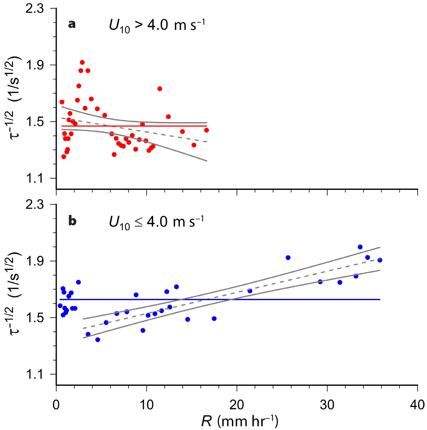
Figure 5. The dependence of the square root of the decay time constant measured by the active controlled flux technique, τ–1/2, on instantaneous rain rate, R, for times when R > 0.1 mm hr–1 for the 2016 SPURS-2 ACFT measurements. Panel (a) shows data where the wind speed, U10, is greater than 4 m s–1 and (b) shows data when U10 is less than 4 m s–1. The τ–1/2 values have been bin-averaged as a function of R as described in the text. The solid colored line in each plot is the average value of the bin-averaged τ–1/2 data in that plot, and the dashed gray line in each plot is a least-squares linear regression of the ACFT data. The solid gray lines are the confidence intervals (95%) for the linear regression. For U10 > 4.0 m s–1 (upper plot), the regression is for the entire data set with τ–1/2(1/s1/2) = −0.0104R + 1.53 with a coefficient of determination of 0.07. For U10 ≤ 4.0 m s–1 (b) the regression is for R > 3 mm hr–1 and τ–1/2(1/s1/2) = 0.0150R + 1.38 with a coefficient of determination of 0.76. > High res figure
|
For the higher wind speed data class (Figure 5a), there is no clear correlation between R and τ–1/2: the data fall around the solid line that represents τ–1/2 averaged over all rain rates. A least-squares linear regression of τ–1/2 with R for the data has a negative slope, suggesting that at higher wind speeds the presence of rain decreases turbulence at the ocean surface. However, the slope is not statistically significant from zero, as shown by the confidence intervals in the plot. In contrast to the data for U10 > 4 m s–1, the lower wind speed data (Figure 5b) show that for R > 3 mm hr–1, rain increases τ–1/2, and that there is a linear relationship between R and τ–1/2. This is consistent with the results of Harrison et al. (2012) from a wind-wave tunnel using a rain simulator. They found that rain had a negligible impact on air-water gas exchange above wind speeds of 5 m s–1. (Note that the lower bound for the regressions in Figure 5 was chosen based on the qualitative observation from Figure 3 showing rain events with R < 5 mm hr–1 did not cause an increase in τ–1/2.)
The low wind speed data in Figure 5b show that the effect of rain on τ–1/2 is relatively small. The time series of τ–1/2 in Figure 3c shows that although each peak in R is correlated with a corresponding increase in τ–1/2, there are temporal offsets between the peaks. This could reflect differences in response times of each measurement, as the ACFT will track changes in local rain rate that occur as fast as the 2 s spacing between pulses from the CO2 laser. However, rain rate was measured using a capacitance accumulation rain gauge, which has a response time that is on order of several minutes. In a rainstorm with sudden bursts of rain, the maximum value for τ–1/2 measured by ACFT could precede the maximum rain rate. This would decrease the apparent effect of rain on surface turbulence when binned as done for the data in Figure 5.
For the low wind case (Figure 5b), it is not clear why the τ–1/2 values decrease from the lowest rain rates up to R = 3 mm hr–1. However, any rain rate below 3 mm hr–1 would be characterized as light rain, which is not expected to be composed of large raindrops that can impart high levels of kinetic energy to the water surface. Therefore, it is likely the increase in τ–1/2 as R decreases from 3 mm hr–1 to 0.1 mm hr–1 is not due to rain-related processes but rather might be an artifact of turbulence generated by internal waves as shown in Figure 2.
Conclusions
These results suggest that ACFT is useful for estimating relative levels of turbulence in the top centimeter of the ocean. The rain-free case in Figure 2 provides further evidence that when a diurnal warm layer is present, internal waves generate mixing and turbulence at the ocean surface. The ACFT measurements made in the presence of rain, the results of which are shown in Figures 3 and 5, demonstrate that rain has a measurable effect on turbulence in the upper centimeter of the ocean, but that this effect diminishes as wind speed increases. The decreased importance of rain relative to wind in generating turbulence supports the conclusions of Harrison et al. (2012), who used laboratory measurements to show that rain was not a significant source of turbulence as wind speed increased above 5 m s–1.
The data shown here represent half of the total ACFT measurements taken during the SPURS-2 field experiments. ACFT was also used during the 2017 SPURS-2 field experiment, and those data can be used to confirm and extend the present findings. Although not discussed here, data for turbulence at the ocean surface is also available for the SPURS-2 time period through temperature and conductivity microstructure measurements that were made at a depth of 0.35 m using instruments mounted on the SSP. Comparison of the ACFT turbulence estimates from the top centimeter with the microstructure turbulence data will provide further insight into the behavior and relevance of rain-generated turbulence at the ocean surface.